Leader Reward for POMO-Based Neural Combinatorial Optimization
May 22, 2024
Abstract
Deep neural networks based on reinforcement learning (RL) for solving combinatorial optimization (CO) problems are developing rapidly and have shown a tendency to approach or even outperform traditional solvers. However, existing methods overlook an important distinction: CO problems differ from other traditional problems in that they focus solely on the optimal solution provided by the model within a specific length of time, rather than considering the overall quality of all solutions generated by the model. In this paper, we propose Leader Reward and apply it during two different training phases of the Policy Optimization with Multiple Optima (POMO) [1] model to enhance the model’s ability to generate optimal solutions. This approach is applicable to a variety of CO problems, such as the Traveling Salesman Problem (TSP), the Capacitated Vehicle Routing Problem (CVRP), and the Flexible Flow Shop Problem (FFSP), but also works well with other POMO-based models or inference phase’s strategies. We demonstrate that Leader Reward greatly improves the quality of the optimal solutions generated by the model. Specifically, we reduce the POMO’s gap to the optimum by more than 100 times on TSP100 with almost no additional computational overhead.
1 Introduction↩︎
Efficient methods for solving combinatorial optimization (CO) problems are widely used in industry, including in deliveries, vehicle routing, production scheduling processes, and other real-world scenarios, all of which hold significant value. However, many CO problems are NP-hard, which means they cannot be quickly solved to an optimal solution. Heuristic solvers such as LKH [2], [3] and HGS [4] have been proposed and are designed by experts based on domain knowledge tailored to specific problems. However, they are less efficient at solving larger-scale CO problems.
Recently, an increasing amount of work has been proposed that uses neural networks to solve CO problems like the Traveling Salesman Problem (TSP) and the Capacitated Vehicle Routing Problem (CVRP), namely Neural Combinatorial Optimization (NCO) [5]. These works mainly consist of methods based on supervised learning (SL) and reinforcement learning (RL). While SL-based methods require a large amount of labeled data, which is time-consuming for the solver to provide, RL-based methods are more attractive and promising. They not only do not rely on the expert’s domain knowledge and labeled datasets, but also are capable of providing high-quality approximate solutions in a short time.
One of the RL-based methods is the construction method, which utilizes transformer architecture [6] to generate solutions sequentially through a decoder. It computes the reward function and uses the REINFORCE algorithm [7] to train the model. POMO [1] takes advantage of the symmetry in the CO problems. They solve the same CO problem from different perspectives and propose a new baseline suitable for the REINFORCE algorithm, which greatly reduces variance and improves the stability of training, making it one of the mainstream approaches. Several subsequent works have adopted it and, based on POMO, have optimized the performance of the inference phase or improved the model’s ability to generalize across distributions and scales. Some other works apply this approach to other CO problems like the flexible flow shop problem (FFSP) and the asymmetric traveling salesman problem (ATSP).
However, such a routine does not take the special aspects of the CO problem into account. For a given CO problem, it focuses only on the optimal solution among all the solutions provided by the model after a period of inference, regardless of the quality of the other solutions. Thus, a good NCO model should value the quality of the best solution (Leader) among all the solutions given, rather than the average quality of all solutions generated. Moreover, when the model repeatedly infers the same problem, it should be able to explore more new solutions, even if the average quality of the solutions produced by each inference might decrease as a result.
In this paper, we propose Leader Reward, which changes the advantage function in the REINFORCE algorithm, and we apply it to two different training phases to motivate the model for more exploration and to place greater emphasis on the leader solution. The implementation of Leader Reward is straightforward, requiring few modifications to POMO’s advantage function and training process. By leveraging the multi-perspective problem-solving properties of POMO, it effectively integrates with POMO-based models and other inference strategies such as Simulation-Guided Beam Search (SGBS) [8] and Efficient Active Search (EAS) [9].
We demonstrate that Leader Reward provides a method to balance exploration and exploitation for POMO. Experimental results indicate that the leader solution often results from stochastic variation, suggesting it is an unbiased, correct, and under-explored direction for the model. We assess the effectiveness of Leader Reward across various CO problems, such as TSP, CVRP, and FFSP, as well as different POMO-based models like MVMoE [10] and Omni-VRP [11]. The results show that Leader Reward significantly enhances model performance with almost no additional computational overhead. Particularly, we reduce POMO’s gap to the optimum by more than 100 times on TSP100, a much greater improvement than that achieved by other studies.
2 Related work↩︎
2.0.0.1 Neural Combinatorial Optimization
The initial attempt to solve CO problems using neural network methods was made by [12]. They proposed the Pointer Network, which selects a member from the input sequence with a pointer and solved the problem of variable-size output dictionaries based on SL. As the model continuously constructs a complete solution from an initial point, it is known as the construction method. [5] suggested using RL for training because SL requires optimal solutions of CO problems as labels. Whereas CO problems are mostly NP-hard and difficult to solve optimally, it is feasible to compute the quality of a solution and design a reward function. [13] proposed AM which modified the model to include attention layers and used the REINFORCE algorithm to train the model, employing a simple greedy rollout as a baseline through the policy gradient. [1] exploited the symmetry in the CO solution representation and proposed POMO which forced the model to solve the same problem from different starting points and used the average of these solutions as the baseline in the REINFORCE algorithm. This approach directly reduces the high variance of different trajectories and improves the training speed and stability of RL.
There is another type of method based on improvement which starts with a random initial solution and iteratively improves it. L2I [14] learn to refine the solution with an operator. NeuRewriter [15] learns a strategy for selecting heuristics and rewrites the current solution. Some other works improve local search or refine strategies [16]–[21]. However, these methods are often limited by search efficiency and high time overhead of inference.
2.0.0.2 POMO-Based Methods
As POMO is a very efficient construction method that can solve hundreds of instances in a few seconds, there has since been a lot of work either exploiting the symmetry of this solution representation or extending and optimizing POMO. [22] applied this symmetry in the CO problem to the MatNet model, making it useful for the FFSP problem and the ATSP problem as well. Sym-NCO [23] exploits symmetries such as rotational invariance and reflection invariance that can greatly improve the generalization of POMO. ELG-POMO [24] devises an auxiliary strategy for learning from local transferable topological features and integrates it with typical construction policies to improve the generality of the model through joint training. Omni-VRP [11] proposed a generic meta-learning framework to simultaneously improve the generalization of models in terms of size and distribution and applied it to POMO.
2.0.0.3 Inference Phase Techniques
There are many techniques applied to the inference phase as well. When a model is trained, these inference techniques can better help the model to find the optimal solution. Active Search [5] can help models to optimize the parameters of the pointer network using RL in the test phase. SGBS [8] is able to examine candidate solutions in a fixed-width tree search. [9] proposed to drastically reduce the time overhead by modifying only a fraction of the model parameters during RL training in the testing phase, known as EAS.
Our method is also based on the symmetry proposed by POMO, as we take advantage of the fact that POMO solves the same problem from different perspectives. This means that our method combines well with POMO-based methods, as well as lots of inference phase techniques, and is able to work together to improve the performance of the model.
3 Preliminary↩︎
Construction-based NCO method is to train a neural network \(\pi_\theta\) with learnable weights \(\theta\). For a CO problem, the model \(\pi_\theta\) can recursively generate a solution (or a trajectory) \(\tau\) using sampling rollout or greedy rollout, denoted as \(\tau \sim \pi_\theta\).
The probability that the model makes an action \(a\) in state \(s\) is denoted as \(\pi_\theta(a|s)\), and the probability that the model generates a solution \(\tau=(a_1, a_2,\dots,a_n)\) can be computed as \(p_\theta(\tau|s) = \prod_{i=1}^n \pi_\theta(a_i|s_i)\). For each solution \(\tau\) generated by the model, the reward for that solution can be computed by the reward function \(R(\tau)\). Note that the reward is only given when the model has finished generating a solution. Given a problem instance \(s\) randomly generated from the problem distribution \(\mathcal{D}\), we want to find the \(\theta\) that maximize the reward \({\operatorname {arg\,max}}_\theta\;\mathbb{E}_{\tau \sim \pi_\theta(s)}(R(\tau))\)
We use the REINFORCE algorithm to learn the weight parameter \(\theta\) of the model. Specifically, we need to maximize the objective function \(\mathcal{L}(\theta) = \mathbb{E}_{\tau \sim \pi_\theta(s)}(R(\tau)-b)\), where \(R(\tau)-b\) is the advantage function, and \(b\) is a baseline which is used to reduce the variance. We use the gradient ascent \(\nabla_\theta \mathcal{L}(\theta) = (R(\tau)-b) \nabla_\theta \log p_\theta ( \tau|s )\) to update the weight parameter \(\theta\) of the model.
4 Methods↩︎
4.1 Leader Reward in the main training phase↩︎
Inspired by POMO, we will solve the same CO problem many times from different perspectives, e.g., the TSP problem will choose different points as starting points, and the FFSP problem will choose different orders for assigning work to the machines. One of the biggest differences between CO problems and other problems is that for a given specific problem, we will only focus on the best of all the solutions, and it does not matter how good the quality of the other solutions given by the model are, except for the best one. This means that the measure of whether a model is good or bad should not be the expected quality of all the solutions given by the model \({\operatorname {arg\,max}}_\theta\;\mathbb{E}_{\tau \sim \pi_\theta(s)}(R(\tau))\), but the expected quality of the best solution after the model solves a particular CO problem multiple times \({\operatorname {arg\,max}}_\theta\;\mathbb{E}_{\tau_1,\dots,\tau_n \sim \pi_\theta(s)}\max(R(\tau_1), R(\tau_2),\dots, R(\tau_n))\). The objective function \(R(\tau) - b\) based on POMO does not allow the model to learn the importance of the leader solution.
We therefore propose the Leader Reward. Specifically, after rolling out a set of trajectories \(\{\tau_1, \tau_2, \cdots, \tau_n\}\) by sampling from the same problem \(s_i\), we compute the new advantage function using the following method:
\[\label{equ1} {{\mathcal{A}_\mathrm{Leader}}}_i^j= \begin{cases} \alpha\times (R(\tau_i^j)-b_i) & \text{if } j=\underset{j}{\operatorname {arg\,max}}(R(\tau^j_i)-b_i)\\ R(\tau^j_i)-b_i & \text{if } j\neq \underset{j}{\operatorname {arg\,max}}(R(\tau^j_i)-b_i). \end{cases}\tag{1}\]
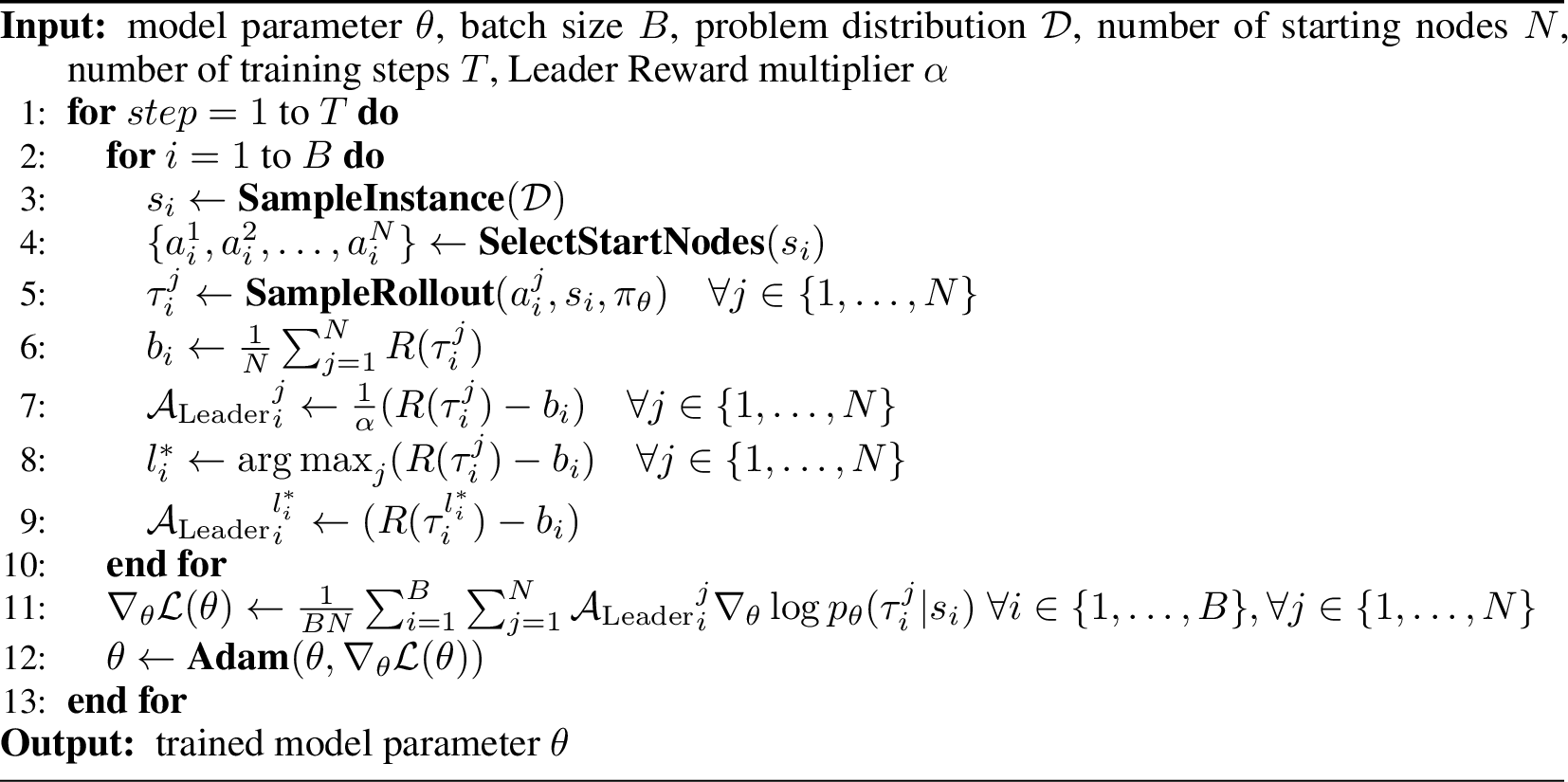
In Equation 1 , \(\alpha>1\), which is a hyperparameter that controls the extra reward earned by the leader. We will take the average reward of all the trajectories sampled from the same problem as the baseline \(b_i\), and then add an extra Leader Reward to the leader trajectory. To maximize the objective function \(\mathcal{L}(\theta)\), we use a gradient ascent as follows:
\[\nabla_\theta \mathcal{L}(\theta) \leftarrow \frac{1}{B N} \sum_{i=1}^B \sum_{j=1}^N{\mathcal{A}_\mathrm{Leader}}_i^j \nabla_\theta \log p_\theta ( \tau_i^j |s_i ),\]
where \(\log p_\theta( \tau_i^j |s_i )\) represents the log probability of sampling the trajectory \(\tau_i^j\), \(B\) is the batch size, and \(N\) is the number of different trajectories sampling from the same problem. Algorithm 1 describes the pseudocode for applying Leader Reward to the training. It is worth noting that in practice, we divide the advantage value for all trajectories by \(\alpha\) (line 7). Since the Adam optimizer is used, multiplying the advantage function by a constant value does not change the result. However, when \(\alpha\) is large, there are some advantages to this approach, which we will explain in Section 4.2.
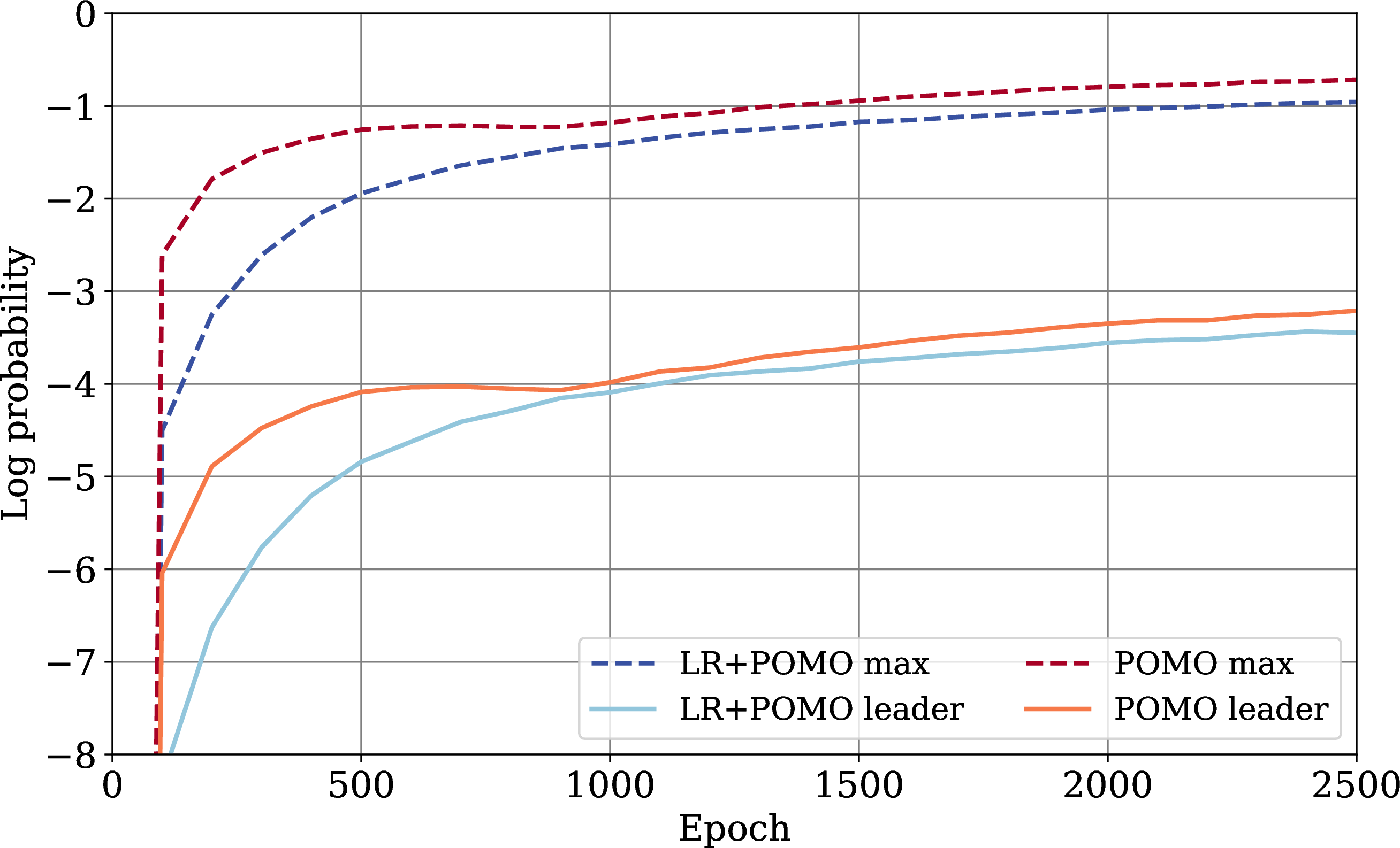
In Figure 2, we show the log probability of generating the leader trajectory and the maximum log probability of 100 trajectories for each TSP100 problem during the training phase. The log probability of the leader trajectory is much smaller than the maximum log probability, implying that it is a low-probability event generated by random sampling and that the model has not yet sufficiently explored it. We also show the results after adding the Leader Reward (LR) during training, which remain the same. This is because all the datasets are randomly generated during the training phase, so no data is reused, thus reducing the risk of overfitting.
4.1.0.1 Proposition 1.
Consider one of the steps during the generation of the solution for the model. Let \(s\) be the state given by the environment at this step, and \(a_i\) be each action the model can take under the state. Let \(\pi_\theta\) be the neural network whose parameters are \(\theta\) and learning rate is \(\gamma\). The probability of each action model can take \(\pi_\theta(a_i | s)\) is calculated from the softmax function \(\sigma(z_i)={e^{z_i}}/({\sum_j e^{z_j}})\) where \(z_i\) represents the score for each decision calculated by the model. The entropy \(H(p)\) of a probability distribution \(p\) over \(n\) actions is given by \(H(p)=-\sum_{i=1}^n p_i \log(p_i)\). Assume \(a^*\) is the learder action and \(\pi_\theta(a^* | s) < -\frac{1}{n}\sum_i\pi_\theta(a_i | s)\), and the new entropy is \(H(p')\) after giving the leader an extra reward \(r\). Then \(H(p') > H(p))\).
See Appendix 7 for the proof. Therefore, Leader Reward is also a way to increase exploration and control the model’s balance between exploration and exploitation by adjusting the size of the value of \(\alpha\). In RL, exploration is crucial for effectively learning how to navigate an environment and make optimal decisions. It can help the model discover new strategies as well as handle sparse rewards. Some traditional methods, such as the Epsilon-Greedy Algorithm [25] will use a hyperparameter \(\epsilon\) to make the model explore randomly with a certain small probability, but the directions explored in this randomized exploration may be sometimes good, sometimes bad. However, the Leader Reward will guide the model in the right direction, as the leader trajectory derived from multiple rollouts of the same problem is a solution free of fluctuations and bias, as well as a new direction not fully explored by the model. This means that the quality of the model’s exploration will be higher than traditional methods.
4.2 Leader Reward in the final training phase↩︎
The distinction in CO problems, which focuses solely on the quality of the optimal solution, not only alters the metrics for evaluating model performance but also modifies the strategies employed by models during inference. When assessing a model’s inferential capabilities, we usually consider the model’s performance across various inference time durations and tailor our method to meet the demands of real-world scenarios. If enough time is available for inference, allowing the model to generate numerous trajectories through sampling rollout, a model that explores diverse potential paths and generates varied solutions will outperform others. Conversely, if the model is afforded only a limited number of attempts or even just a single try at solving a problem due to time constraints, a more robust model is probabilistically favored to provide a reasonably good approximate solution.
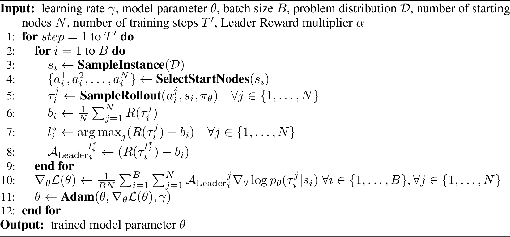
As mentioned in Section 4.1, applying different values of \(\alpha\) during training alters the extent to which the model explores, leading to a final model that tends towards being either aggressive or conservative. This approach can also be employed in the final training phase. Hence, we propose Algorithm 3, a method based on Leader Reward, to adjust the conservativeness of the model. This algorithm could enhance the model’s aggressiveness by setting \(\alpha = +\infty\) and balance the specific degrees of aggression and conservatism by adjusting the learning rate \(\gamma\), ensuring the model converges to an appropriate state. It just requires a small amount of training time, converging in just 100 epochs on TSP100, which is approximately one-thirtieth of the entire training process.
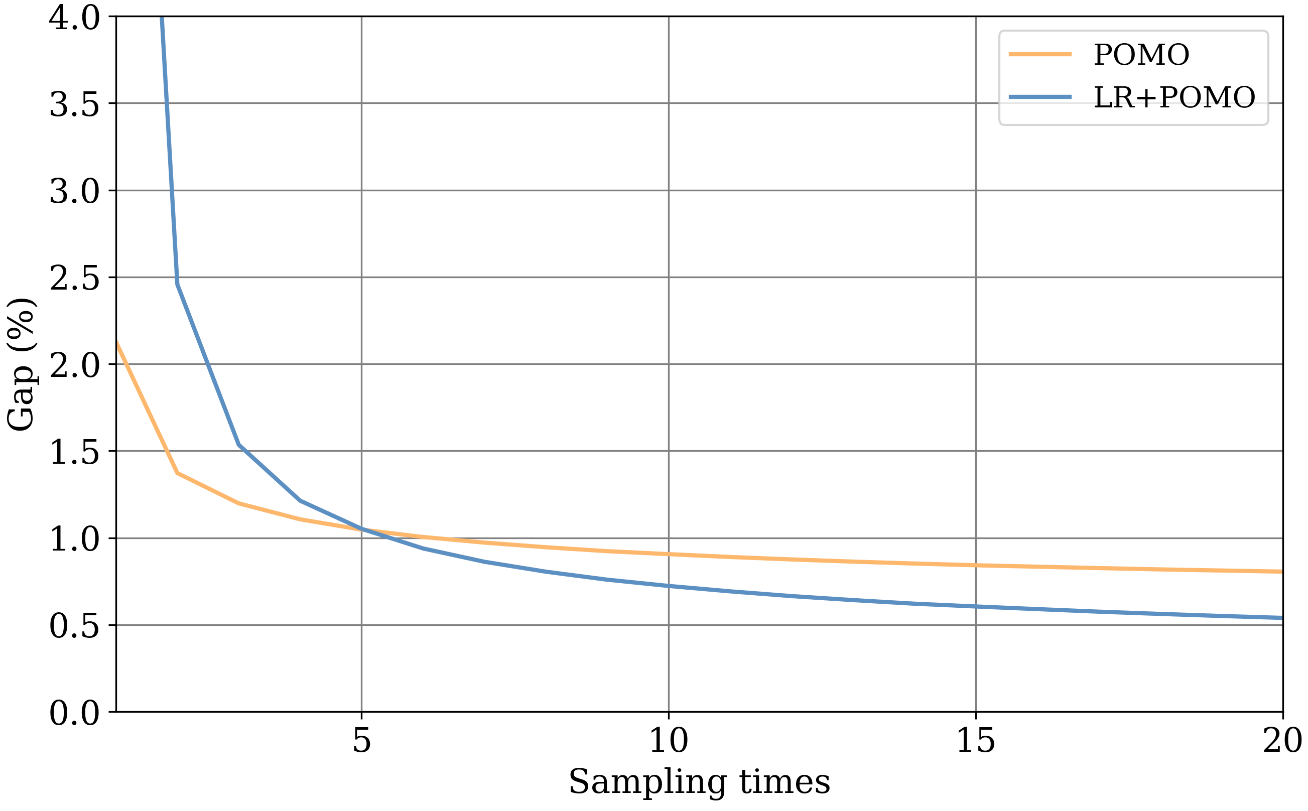
Figure 4 shows the gap between the solutions generated by the model and the optimal solution when applying Algorithm 3 to solve the same problem by sampling multiple times. It is observed that this algorithm results in a decline in the average quality of solutions produced by the model, as the gap of the solution provided by the model escalates from 2.13% to 8.52% when solving the problem just once. This escalation occurs because, when a model solves the same problem only a limited number of times, the emphasis is on the average quality of solutions it provides. Conversely, as the model solves the same problem more frequently, a more aggressive model becomes advantageous.
Given that POMO leverages the symmetry of solution representations and data augmentation, POMO-based methods typically involve solving the same problem a large number of times during the inference phase. Taking the TSP100 as an example, these methods will sample the same problem 800 times. This algorithm is designed to leverage POMO’s capability of repeated problem-solving, enhancing the model’s aggressiveness at the expense of deteriorating the average solution quality. The trade-off aims to improve the probability of generating high-quality, optimal solutions.
4.3 Leader Reward + SGBS + EAS↩︎
As POMO is a highly efficient construction method, recently numerous improvements have been made to enhance its performance. One such improvement is SGBS + EAS, an optimization strategy tailored for the POMO’s inference phase. Our method can also be applied to the inference phase and works well with SGBS + EAS, further reducing the gap between the model’s solution and the optimum.
SGBS is an inference phase technique that enhances the quality of solutions generated by the POMO model. During the solution generation process, it produces \(\beta \times (\gamma-1)\) directions at each step, and retains the best \(\beta\) among them through a greedy rollout mechanism. This method aims to generate the best \(\beta\) solutions at the same time, thereby improving the quality of the solutions generated by the model. Such an algorithm, capable of efficiently producing multiple solutions, enables us to attain a superior solution within a short inference time while also emphasizing the exploratory performance of the model. In contrast to the previous practice of pursuing a single greedy rollout to obtain a nearly approximate solution, we now, with the efficient inference strategy of SGBS, prefer the model to capitalize on the greater opportunities provided by SGBS to fully explore the potential of other solutions.
EAS is a method that trains on a test set by using POMO’s pre-trained model and updates the parameters during testing to enhance performance. It leverages the fact that the problem only requires an optimal solution and, given sufficient inference time, allows for tuning the model during this period. EAS accelerates the training process by updating only a subset of parameters. Since EAS involves training on a test set, it can be integrated with the approach described in Section 4.1. This integration treats EAS as the main training phase and uses Leader Rewards to guide the model in a correct new direction during training.
SGBS and EAS collaborate in a way that SGBS assists EAS by sharing incumbent solutions. SGBS helps EAS escape local optima by discovering superior solutions through efficient generative methods that leverage new paths explored by EAS during training. This method alternates between EAS and SGBS in sequence. However, SGBS has a significant time overhead, as one iteration of SGBS(4,4) on CVRP100 takes about 6 times longer than one iteration of EAS, and one iteration of SGBS(10,10) on TSP100 takes about 20 times longer than one iteration of EAS, which makes this strategy less viable when training time is limited. Experimentally, we found that increasing the number of iterations of EAS improves model performance when time is limited, but at the expense of making the model more likely to fall into a local optimum and perform worse in the long term. However, since EAS operates in the testing phase, where time is precious, we believe that sacrificing a little long-term performance for a reduction in short-term performance is worthwhile.
There are also lots of other works based on POMO, such as MatNet, Omni-VRP, and MVMoE. Our approach is an optimization of the POMO training approach, and we find that it simultaneously benefits these POMO-based models. The experimental results are shown in Section 5. This demonstrates the generalizability of our approach.
5 Experiments↩︎
The training and testing were conducted on a single Nvidia RTX 4090 GPU. To evaluate the effectiveness of Leader Reward (abbreviated as LR in the table), we modified POMO (MIT license) [1] and assessed its performance on the TSP and CVRP problems. We also applied our method to MatNet (MIT license) [22] and tested its performance on the FFSP problem to show our method’s applicability to models that utilize the symmetric representation of solutions in POMO. Since the SGBS+EAS optimization is relevant to all three problems, we also evaluated the performance after implementing SGBS+EAS (MIT license) [8] in the inference phase. To further demonstrate the applicability of our method to other POMO-based models, we tested Leader Reward on two additional models, MVMoE (MIT license) [10] and Omni-VRP (MIT license) [11]. The results can be found in Appendix 10. We also tested the performance of Leader Reward on the realistic datasets TSPLib [26] and CVRPLib [27]; details of these tests can be found in Appendix 11. As some of the results in the table were obtained from different hardware (v3-8 TPU or Nvidia A100 GPUs), we’ve marked their time consumption with \(*\) for a fair comparison.
5.0.0.1 TSP
The TSP problem can be considered one of the benchmark problems among CO problems, and many NCO models are tested for performance on the TSP problem. In the TSP, there are multiple points in a two-dimensional space, and the distance between any two points is measured using Euclidean distance. The goal is to find the minimal distance required to start from any one point, pass through each point exactly once, and return to the starting point. To maintain consistency with previous experiments, we used the test set generated by [8]. Specifically, 10,000 instances of TSP100 were generated using the random seed 1234, and 1,000 instances each of TSP150 and TSP200 were generated using the random seed 1235.
We use the results of exact-solver Concorde [28] as a standard for comparison, and we also give the results of LKH3. For the NCO method, we give results for DPDP [29], COMPASS [30], Poppy [31], and POMO. However, since our optimization is based on POMO, our main emphasis is on the magnitude of improvement in POMO. Just as POMO can be optimized using SGBS+EAS, we also present the results of combining Leader Reward with SGBS+EAS, as well as the results for different lengths of inference time.
As POMO trained a TSP100 model for a total of 3050 epochs, we also kept the overall training time consistent to ensure a fair comparison. Specifically, we use \(\alpha = 40\) when applying Leader Reward in the main training phase and trained POMO for 2900 epochs, in the final training phase we set \(\alpha = +\infty\) trained for 150 epochs. In the inference phase, we combined Leader Reward with SGBS+EAS. We selected the hyperparameters \(\beta = 10\) and \(\gamma = 10\) for SGBS. For EAS, we set the parameter of Leader Reward to \(\alpha=40\) and performed SGBS after every 20 EAS iterations.
Table 1 shows the performance of Leader Reward on the TSP problem. The result for LR+SGBS is not included in the table because we found that LR+SGBS+EAS performs better than LR+SGBS in terms of both time consumption and the gap. It can be found that Leader Reward can significantly improve the performance and generalization of the POMO model on the TSP. Specifically, Leader Reward reduces the POMO’s gap to the optimum by 10 times, and can be boosted up to 200 times when optimized with SGBS+EAS inference strategy. For generalization capabilities, Leader Reward can also reduce the gap by 97% and 84% on TSP150 and TSP200, respectively, which represents a huge improvement greater than that achieved by other studies.
| Method | Test (10K instances) | Generalization (1K instances) | |||||||
| TSP100 | TSP150 | TSP200 | |||||||
| Cost | Gap | Time | Cost | Gap | Time | Cost | Gap | Time | |
| Concorde | 7.765 | - | 82m | 9.346 | - | 17m | 10.687 | - | 31m |
| LKH3 | 7.765 | 0.000% | 8h | 9.346 | 0.000% | 99m | 10.687 | 0.000% | 3h |
| Poppy 16 | 7.770 | 0.07% | 1m* | 9.372 | 0.27% | 20s* | |||
| POMO | 7.776 | 0.144% | 1m | 9.397 | 0.544% | 14s | 10.843 | 1.459% | 31s |
| LR+POMO | 7.766 | 0.014% | 1m | 9.364 | 0.193% | 14s | 10.792 | 0.985% | 31s |
| POMO(sampling) | 7.771 | 0.078% | 3h* | 9.378 | 0.355% | 1h* | 10.838 | 1.417% | 3h* |
| DPDP | 7.765 | 0.004% | 2h* | 9.434 | 0.937% | 44m* | 11.154 | 4.370% | 74m* |
| COMPASS | 7.765 | 0.002% | 2h* | 9.350 | 0.043% | 32m* | 10.723 | 0.337% | 70m* |
| SGBS+EAS(short) | 7.770 | 0.063% | 37m | 9.368 | 0.236% | 11m | 10.764 | 0.718% | 29m |
| SGBS+EAS | 7.768 | 0.045% | 2h | 9.359 | 0.142% | 2h | 10.739 | 0.484% | 2h |
| LR+SGBS+EAS(short) | 7.765 | 0.0007% | 25m | 9.347 | 0.009% | 17m | 10.701 | 0.133% | 37m |
| LR+SGBS+EAS | 7.765 | 0.0002% | 2h | 9.346 | 0.005% | 2h | 10.695 | 0.075% | 2h |
5.0.0.2 CVRP
In the CVRP, multiple points are distributed across a two-dimensional space, each associated with a demand value. A vehicle may depart from the depot multiple times, pass through some of these points, and then return to the depot. The total demand of the points visited in each trip must not exceed the vehicle’s capacity. The goal is to find the shortest route that ensures each point is visited at least once.
We used the same test set setup as in the TSP problem, and we used the results of the heuristic solver HGS [32], [33] as the baseline for comparison. For the training process, we used \(\alpha = 10\) when applying Leader Reward in the main training phase and trained the POMO model for 28,500 epochs, and in the final training phase, we set \(\alpha = +\infty\). In the inference phase, we selected the hyperparameters \(\beta=4\) and \(\gamma=4\) for SGBS. For EAS, we set the parameter of Leader Reward to \(\alpha=10\) and performed SGBS after every 3 EAS iterations.
Table 2 displays the performance of Leader Reward on the CVRP problem. It is evident that Leader Reward enhances both the performance and generalization of the POMO model on this problem, reducing the gap by 35%, 27%, and 40% for CVRP100, CVRP150, and CVRP200, respectively.
5.0.0.3 FFSP
To demonstrate the applicability of Leader Reward to models that leverage the symmetry of the solution representation, we also applied it to MatNet and tested the performance on the FFSP problem.
The FFSP problem is modeled on the production scheduling process in a real manufacturing application, where each job must be performed sequentially across \(S\) stages. Each stage has \(M\) types of machines, and each job takes a different amount of time on each machine. Within the same stage, it is only necessary to work on any one of the \(M\) types of machines. The goal of the problem is to find the shortest possible time required to complete all jobs.
To maintain consistency with previous experiments, we used \(S=3\) and \(M=4\), and the possible time required for each job was a random integer from 2 to 9. We used the test set generated by [22] and tested how the model performed with \(N=\{20,50,100\}\) jobs. To ensure that the total training time is consistent, we chose \(\alpha=\{4, 4, 2\}\) and trained MatNet for \(\{50, 100, 150\}\) epochs. In the inference phase, we selected the hyperparameters \(\beta=5\) and \(\gamma=6\) for SGBS, and we performed SGBS after every 3 EAS iterations. We also give results for mixed-integer programming models CPLEX, and other heuristics methods.
Results in Table 3 show that the Leader Reward method outperforms both heuristic methods and NCO methods in solving the FFSP problem and significantly improves the performance of MatNet, demonstrating the effectiveness of our method for MatNet.
| Method | Test (10K instances) | Generalization (1K instances) | |||||||
| CVRP100 | CVRP150 | CVRP200 | |||||||
| Cost | Gap | Time | Cost | Gap | Time | Cost | Gap | Time | |
| HGS | 15.563 | - | 24h | 19.052 | - | 5h | 21.755 | - | 9h |
| LKH3 | 15.646 | 0.532% | 6d | 19.222 | 0.891% | 20h | 22.003 | 1.138% | 25h |
| Poppy 32 | 15.73 | 1.072% | 5m* | 19.50 | 2.350% | 1m* | |||
| POMO | 15.754 | 1.228% | 1m | 19.686 | 3.324% | 16s | 23.057 | 5.983% | 34s |
| LR+POMO | 15.729 | 1.064% | 1m | 19.682 | 3.306% | 16s | 23.012 | 5.775% | 34s |
| POMO(sampling) | 15.663 | 0.641% | 6h* | 19.478 | 2.235% | 2h* | 23.176 | 6.530% | 5h* |
| DPDP | 15.627 | 0.410% | 23h* | 19.312 | 1.363% | 5h* | 22.263 | 2.333% | 9h* |
| COMPASS(no aug) | 15.594 | 0.198% | 4h* | 19.313 | 1.369% | 2h* | 22.462 | 3.248% | 2h* |
| SGBS+EAS(short) | 15.605 | 0.271% | 2h | 19.227 | 0.920% | 1h | 22.274 | 2.382% | 3h |
| SGBS+EAS | 15.587 | 0.152% | 10h | 19.154 | 0.532% | 3h | 22.109 | 1.626% | 7h |
| LR+SGBS+EAS(short) | 15.588 | 0.158% | 2h | 19.160 | 0.566% | 1h | 22.106 | 1.611% | 3h |
| LR+SGBS+EAS | 15.579 | 0.099% | 10h | 19.126 | 0.389% | 3h | 21.966 | 0.967% | 7h |
| FFSP20 | FFSP50 | FFSP100 | |||||||
| Cost | Gap | Time | Cost | Gap | Time | Cost | Gap | Time | |
| CPLEX(60s) | 46.37 | 91.857% | 17h | \(\times\) | \(\times\) | ||||
| CPLEX(600s) | 36.56 | 51.268% | 167h | ||||||
| Genetic Algorithm | 30.57 | 26.484% | 56h | 56.37 | 16.851% | 128h | 98.69 | 12.036% | 232h |
| Particle Swarm Opt. | 29.07 | 20.278% | 104h | 55.11 | 14.239% | 208h | 97.32 | 10.480% | 384h |
| MatNet | 25.392 | 5.060% | 2m | 49.600 | 2.817% | 5m | 89.745 | 1.881% | 13m |
| LR+MatNet | 25.232 | 4.398% | 2m | 49.363 | 2.326% | 5m | 89.207 | 1.270% | 13m |
| MatNet(sampling) | 24.60 | 1.783% | 10h* | 48.78 | 1.117% | 20h* | 88.95 | 0.979% | 40h* |
| SGBS+EAS(short) | 24.467 | 1.233% | 3h | 48.837 | 1.235% | 6h | 88.980 | 1.013% | 10h |
| SGBS+EAS | 24.250 | 0.335% | 15h | 48.519 | 0.576% | 30h | 88.568 | 0.545% | 60h |
| LR+SGBS+EAS(short) | 24.395 | 0.935% | 3h | 48.596 | 0.736% | 6h | 88.455 | 0.417% | 10h |
| LR+SGBS+EAS | 24.169 | - | 15h | 48.241 | - | 30h | 88.088 | - | 60h |
6 Conclusion and Discussion↩︎
In this paper, we propose a new advantage function, Leader Reward, applicable to the POMO model and other models that leverage the symmetry of this solution representation. We analyze the specificity of the CO problem and apply Leader Reward during two different phases of training to improve models’ performance. Experiments show that this method performs well on various CO problems (TSP, CVRP, FFSP) and with different POMO-based models (MatNet, Omni-VPR, MVMoE). It is capable of further improving the model’s performance using inference strategies. Moreover, this performance enhancement incurs almost no additional computational overhead.
For potential societal impacts, we believe that the CO problem is closely related to practical challenges such as deliveries, vehicle routing, and production scheduling. With the development of NCO, models that provide solutions with greater accuracy and in less time can significantly enhance the efficiency of societal and productive activities. Therefore, we believe that the societal impacts of our work are mainly positive, with generally no negative societal impacts. In future work, we will attempt to dynamically adjust the parameter \(\alpha\) in the Leader Reward, aiming to better integrate it with other models and inference strategies.
Our code for the experiments can be found in the supplementary material.
7 Proof↩︎
Proof. Assume there are \(n\) actions \(\{z_1, z_2,\dots,z_n\}\) and the leader action is \(z_1\). The probability of each actions chosen by model \(\displaystyle p_i=\sigma(z_i)= \frac{e^{z_i}}{{\sum_{j=1}^n e^{z_j}}}\) and \(p_1<-\frac{1}{n}\sum_i p_i\).
We have that
\[\frac{\partial p_i}{\partial z_j} = p_i\cdot(\delta_{ij}-p_j),\]
where \(\delta_{ij}\) is the Kronecker delta. The entropy is calculate by \(H(p) = -\sum_{i=1}^n p_i\log(p_i)\).
As the original proposition is equivalent to \(\frac{\partial H(p)}{\partial z_1} >0\), we have that
\[\begin{align} \frac{\partial H(p)}{\partial z_1} &= \sum_{i=1}^n \frac{\partial H(p)}{\partial p_i}\cdot \frac{\partial p_i}{\partial z_1} \\ &= \frac{\partial H(p)}{\partial p_1}\cdot \frac{\partial p_1}{\partial z_1} + \sum_{i=2}^n \frac{\partial H(p)}{\partial p_i}\cdot \frac{\partial p_i}{\partial z_1} \\ &= (-\ln p_1 -1)\cdot p_1\cdot(1-p_1) + \sum_{i=2}^n (-\ln p_i -1)\cdot p_i(-p_1)) \\ &= p_1\cdot(- \ln p_1 +\sum_{i=1}^n p_i \ln p_i ) \\ &= p_1\cdot(- \ln p_1 -H(p)). \\ \end{align}\]
As the sum of the probabilities of all actions \(p_1+p_2+\cdots+p_n =1\) , we have that
\[\begin{align} \frac{\partial H(p)}{\partial z_1} &= p_1\cdot(- \ln p_1 -H(p)) \\ &= p_1\cdot(- (p_1+p_2+\cdots+p_n)\cdot\ln p_1 -H(p)). \\ \end{align}\]
The entropy \(H(p)\) will be maximum if and only if \(p_2=p_3=\cdots=p_n=\frac{1-p_1}{n-1}\), which implies that
\[\begin{align} \frac{\partial H(p)}{\partial z_1} &= p_1\cdot(- (p_1+p_2+\cdots+p_n)\cdot\ln p_1 -H(p)) \\ &> p_1\cdot(- (p_1+p_2+\cdots+p_n)\cdot\ln p_1 +p_1\ln p_1 + \frac{1-p_1}{n-1}\cdot\sum_{i=2}^n \ln \frac{1-p_1}{n-1}) \\ &= p_1\cdot(- (p_1+(n-1)\cdot \frac{1-p_1}{n-1})\cdot\ln p_1 +p_1\ln p_1 + \frac{1-p_1}{n-1}\cdot(n-1)\cdot \ln \frac{1-p_1}{n-1}) \\ &= p_1\cdot (1-p_1) \cdot(\ln \frac{1-p_1}{n-1} - \ln p_1) >0. \\ \end{align}\] ◻
8 Hyperparameter Experiments↩︎
8.1 Hyperparameter for the main training phase↩︎
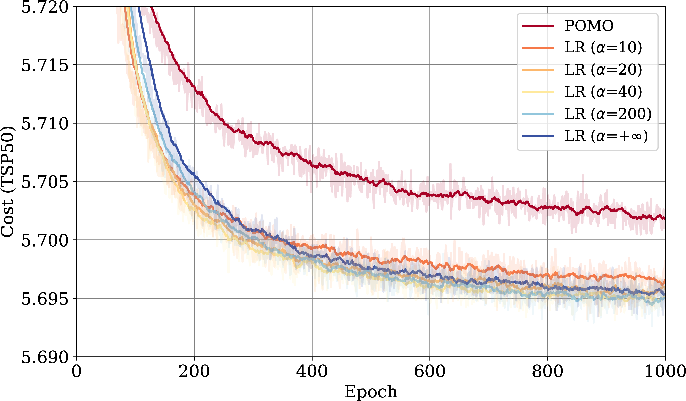
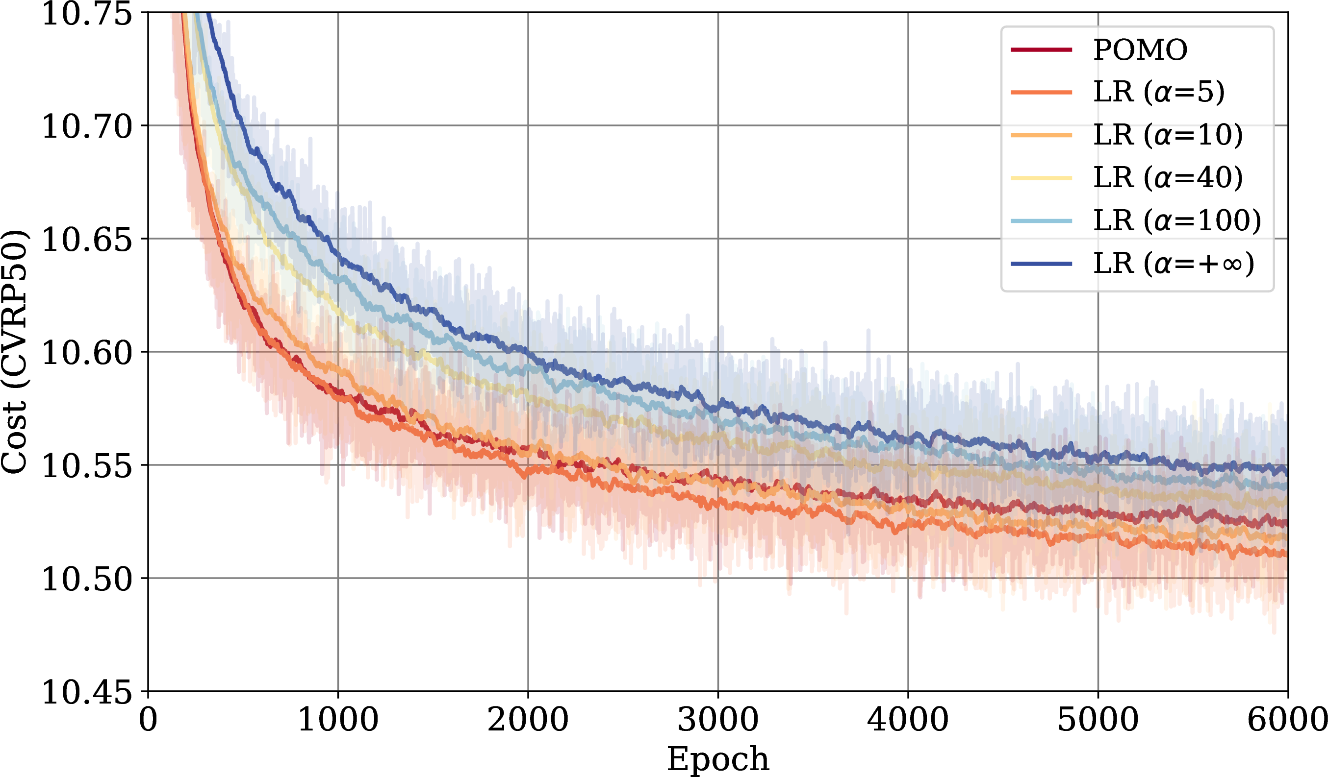
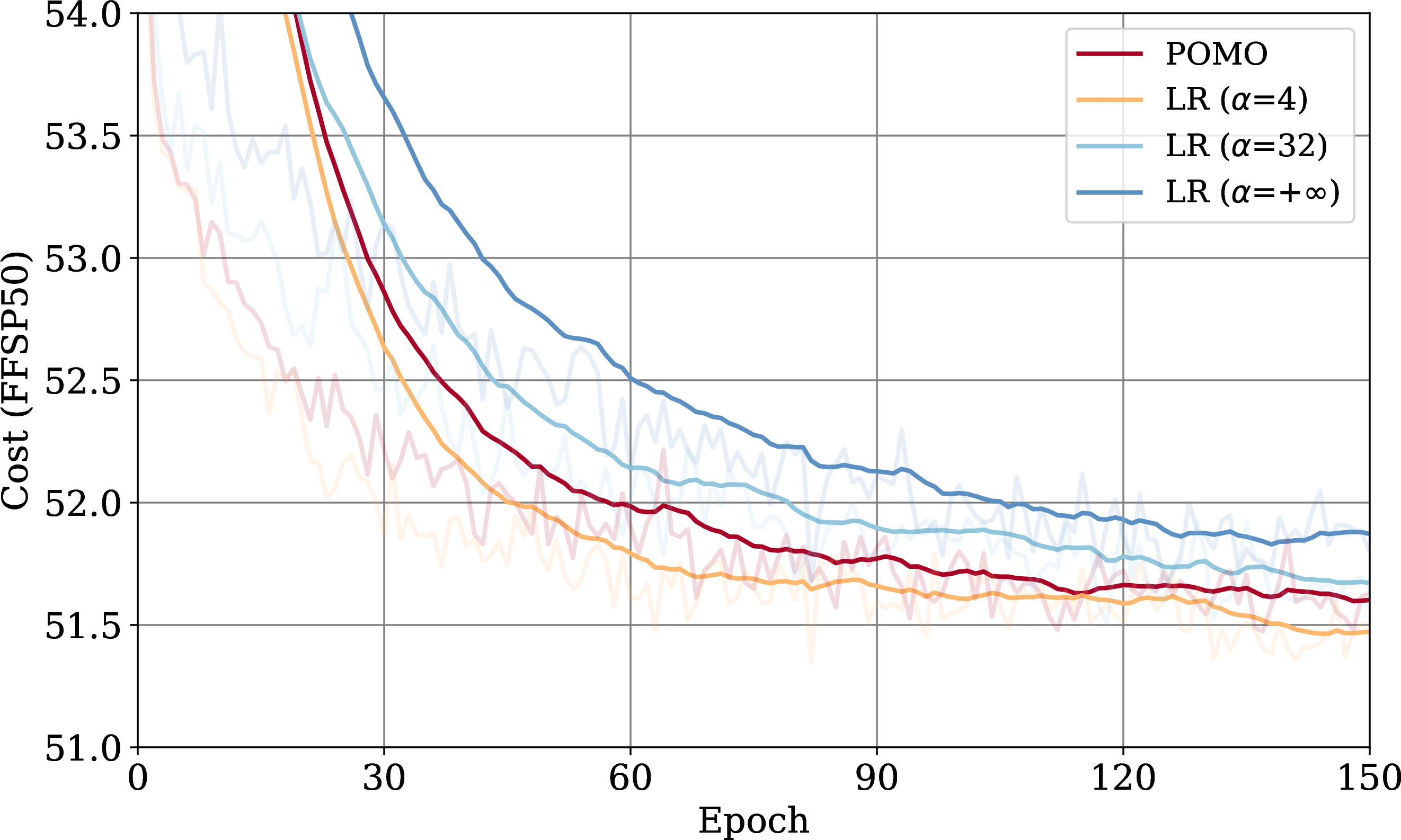
Figure 5: Comparison of learning curves when choosing different \(\alpha\) for Leader Reward during the main training phase on the TSP, CVRP, and FFSP problem.. a — TSP50, b — CVRP50, c — FFSP50
Figure 5 shows the learning curves on the TSP, CVRP, and FFSP problem in the case of using different \(\alpha\) as a parameter for Leader Reward in the main training phase. As experiments on problems of size 100 would be too computationally expensive, we give the results for problems of size 50. In TSP, Leader Reward can give a large boost to POMO’s performance and is robust to the hyperparameter \(\alpha\). As \(\alpha\) increases, the model gradually converges better, but there is a little negative lift when \(\alpha\) is particularly large. In CVRP and FFSP, using too large an \(\alpha\) will make the model perform worse instead. As we need to balance the exploration and exploitation of the model, a proper \(\alpha\) will make the best use of Leader Reward’s performance.
We also notice that Poppy [31] proposed the policy gradient for populations, which is a little bit like setting \(\alpha = +\infty\) in the Leader Reward when training only one population. However, as shown in the figure, this training method leads to poor model performance. Therefore, we consider poppy and Leader Reward to be two different methods, with the former emphasizing performance improvement through large populations and the latter emphasizing making the model value the leader.
8.2 Hyperparameter for the final training phase↩︎
In this section, we test the results of applying Leader Reward to POMO only in the final training phase. Table 4 shows the expected value of the cost, the mean, and the variance of 100 trajectories sampled from the TSP100 problem when choosing different learning rates \(\gamma\). The results show that our method has higher robustness to \(\gamma\), as the costs drop dramatically (from 0.32% to about 0.11%) as long as \(\gamma\) is within a reasonable range.
It’s worth noting that our method can significantly increase the variance of solutions (from about 0.05 to about 0.3) and ultimately improve the performance of the model, at the cost of reducing the average quality of the solution. Therefore, controlling \(\gamma\) within a reasonable range can maximize the performance of this method.
| Method | Cost(no aug.) | Gap | Mean \((\mu)\) | Variance \((\sigma)\) |
|---|---|---|---|---|
| POMO | 7.7891 | 0.316% | 7.837 | 0.048 |
| LR \((\gamma=1\times10^{-5})\) | 7.7739 | 0.121% | 7.904 | 0.229 |
| LR \((\gamma=5.5\times10^{-5})\) | 7.7726 | 0.104% | 7.938 | 0.314 |
| LR \((\gamma=1\times10^{-4})\) | 7.7728 | 0.106% | 7.955 | 0.349 |
| LR \((\gamma=1.5\times10^{-4})\) | 7.7733 | 0.113% | 7.974 | 0.379 |
9 Ablation Study↩︎
In order to demonstrate the effectiveness of Leader Reward in both phases, we further conduct an ablation study. Table 5 shows the cost and the gap in TSP, CVRP, and FFSP problems after removing some of the phases. The results show that both phases play a key role in improving the performance of the model.
| Method | TSP100 | CVRP100 | FFSP100 | |||
| Cost | Gap | Cost | Gap | Cost | Gap | |
| LR | 7.766 | 0.014% | 15.729 | 1.064% | 89.207 | 1.270% |
| w/o main phase | 7.766 | 0.025% | 15.732 | 1.085% | 89.294 | 1.369% |
| w/o final phase | 7.768 | 0.040% | 15.748 | 1.191% | 89.406 | 1.496% |
| w/o both phase | 7.776 | 0.144% | 15.754 | 1.228% | 89.745 | 1.881% |
10 Results on other POMO-based models↩︎
We further implement our method on MVMoE [10] and Omni-VRP [11]. We follow the default setting of the authors and the only change is applying Leader Reward to the advantage function during training. In both models, we set \(\alpha=5\) during the main phase. We also report the performance when the final phase is removed. As shown in Table 6 and Table 7, both phases bring significant improvement in performance.
| Problem | MVMoE | LR w/o final phase | LR | |||
| Cost | Gap | Cost | Gap | Cost | Gap | |
| CVRP | 10.427 | 0.890% | 10.423 | 0.846% | 10.416 | 0.785% |
| OVRP | 6.657 | 2.418% | 6.647 | 2.265% | 6.625 | 1.937% |
| VRPB | 8.167 | 1.495% | 8.159 | 1.395% | 8.149 | 1.275% |
| VRPL | 10.501 | 0.087% | 10.496 | 0.039% | 10.486 | -0.057% |
| VRPTW | 15.000 | 3.412% | 14.985 | 3.293% | 14.955 | 3.088% |
| OVRPTW | 8.964 | 3.217% | 8.941 | 2.949% | 8.916 | 2.662% |
| OVRPB | 6.111 | 6.333% | 6.093 | 6.016% | 6.065 | 5.536% |
| OVRPL | 6.653 | 2.502% | 6.641 | 2.323% | 6.624 | 2.053% |
| VRPBL | 8.175 | 1.808% | 8.162 | 1.655% | 8.151 | 1.513% |
| VRPBTW | 16.019 | 8.589% | 15.986 | 8.364% | 15.952 | 8.137% |
| VRPLTW | 14.927 | 2.362% | 14.913 | 2.253% | 14.888 | 2.071% |
| OVRPBL | 6.098 | 6.215% | 6.077 | 5.856% | 6.054 | 5.445% |
| OVRPBTW | 9.490 | 9.350% | 9.472 | 9.139% | 9.449 | 8.877% |
| OVRPLTW | 8.965 | 3.385% | 8.942 | 3.125% | 8.916 | 2.824% |
| VRPBLTW | 15.941 | 8.748% | 15.932 | 8.686% | 15.897 | 8.448% |
| OVRPBTW | 9.514 | 9.644% | 9.484 | 9.298% | 9.457 | 8.976% |
| (Size, Distribution) | Omni-VRP | LR w/o final phase | LR | |||
| Cost | Gap | Cost | Gap | Cost | Gap | |
| \((200, GM_2^5)\) | 9.027 | 2.773% | 8.991 | 2.353% | 8.965 | 2.068% |
| \((200, R)\) | 8.372 | 2.124% | 8.341 | 1.756% | 8.329 | 1.610% |
| \((200, E)\) | 8.240 | 1.845% | 8.216 | 1.546% | 8.215 | 1.528% |
| \((300, U)\) | 13.400 | 3.442% | 13.342 | 2.995% | 13.329 | 2.892% |
| \((300, GM_3^{10})\) | 9.845 | 3.941% | 9.797 | 3.439% | 9.784 | 3.307% |
| \((300, GM_7^{50})\) | 5.787 | 2.714% | 5.770 | 2.420% | 5.761 | 2.257% |
| \((300, R)\) | 10.162 | 3.774% | 10.114 | 3.287% | 10.101 | 3.149% |
| \((300, E)\) | 9.801 | 3.384% | 9.764 | 2.989% | 9.765 | 3.007% |
| \((500, R)\) | 13.428 | 8.366% | 13.356 | 7.788% | 13.315 | 7.459% |
| \((500, E)\) | 12.672 | 7.996% | 12.616 | 7.519% | 12.589 | 7.286% |
| \((1000, R)\) | 20.374 | 19.214% | 20.348 | 19.072% | 20.101 | 17.625% |
| \((1000, E)\) | 18.575 | 18.629% | 18.567 | 18.584% | 18.397 | 17.502% |
11 Results on TSPLib and CVRPLib↩︎
This section gives a performance evaluation of our method on TSPLib [26] and CVRPLib [27], where we choose instances with size \(N<250\). Both POMO and our model are pre-trained on \(N=100\) and evaluated in Table 1 and Table 2. In this experiment, we report results under greedy strategy and instance augmentation. As shown below, our method outperforms POMO on both datasets. See Table 8 and Table 9.
| Instance | Optimal | POMO | LR+POMO | ||
| Cost | Gap | Cost | Gap | ||
| berlin52 | 7542 | 7545 | 0.04% | 7544 | 0.03% |
| bier127 | 118282 | 128660 | 8.77% | 120606 | 1.96% |
| ch130 | 6110 | 6120 | 0.16% | 6117 | 0.11% |
| ch150 | 6528 | 6562 | 0.52% | 6559 | 0.47% |
| d198 | 15780 | 18508 | 17.29% | 18967 | 20.20% |
| eil101 | 629 | 641 | 1.91% | 640 | 1.75% |
| eil51 | 426 | 430 | 0.94% | 429 | 0.70% |
| eil76 | 538 | 544 | 1.12% | 544 | 1.12% |
| kroA100 | 21282 | 21370 | 0.41% | 21285 | 0.01% |
| kroA150 | 26524 | 26709 | 0.70% | 26783 | 0.98% |
| kroA200 | 29368 | 29831 | 1.58% | 30088 | 2.45% |
| kroB100 | 22141 | 22212 | 0.32% | 22210 | 0.31% |
| kroB150 | 26130 | 26435 | 1.17% | 26331 | 0.77% |
| kroB200 | 29437 | 29876 | 1.49% | 30004 | 1.93% |
| kroC100 | 20749 | 20787 | 0.18% | 20760 | 0.05% |
| kroD100 | 21294 | 21473 | 0.84% | 21412 | 0.55% |
| kroE100 | 22068 | 22167 | 0.45% | 22137 | 0.31% |
| lin105 | 14379 | 14454 | 0.52% | 14419 | 0.28% |
| pr107 | 44303 | 44585 | 0.64% | 44663 | 0.81% |
| pr124 | 59030 | 59246 | 0.37% | 59075 | 0.08% |
| pr136 | 96772 | 97521 | 0.77% | 97562 | 0.82% |
| pr144 | 58537 | 58802 | 0.45% | 59403 | 1.48% |
| pr152 | 73682 | 74596 | 1.24% | 75218 | 2.08% |
| pr226 | 80369 | 83281 | 3.62% | 87103 | 8.38% |
| pr76 | 108159 | 108159 | 0.00% | 108159 | 0.00% |
| rat195 | 2323 | 2512 | 8.14% | 2432 | 4.69% |
| rat99 | 1211 | 1234 | 1.90% | 1224 | 1.07% |
| rd100 | 7910 | 7910 | 0.00% | 7910 | 0.00% |
| st70 | 675 | 677 | 0.30% | 677 | 0.30% |
| ts225 | 126643 | 132623 | 4.72% | 128711 | 1.63% |
| tsp225 | 3861 | 4111 | 6.48% | 4093 | 6.01% |
| u159 | 42080 | 42480 | 0.95% | 42460 | 0.90% |
| Avg Gap | 2.12% | 1.95% | |||
| Instance | Optimal | POMO | LR+POMO | ||
| Cost | Gap | Cost | Gap | ||
| X-n247-k50 | 37274 | 42420 | 13.81% | 44217 | 18.63% |
| X-n242-k48 | 82751 | 89185 | 7.78% | 89669 | 8.36% |
| X-n237-k14 | 27042 | 31272 | 15.64% | 29363 | 8.58% |
| X-n233-k16 | 19230 | 21119 | 9.82% | 20979 | 9.10% |
| X-n228-k23 | 25742 | 29354 | 14.03% | 28758 | 11.72% |
| X-n223-k34 | 40437 | 43804 | 8.33% | 43877 | 8.51% |
| X-n219-k73 | 117595 | 122208 | 3.92% | 124756 | 6.09% |
| X-n214-k11 | 10856 | 11763 | 8.35% | 11741 | 8.15% |
| X-n209-k16 | 30656 | 32399 | 5.69% | 32410 | 5.72% |
| X-n204-k19 | 19565 | 20976 | 7.21% | 21284 | 8.79% |
| X-n200-k36 | 58578 | 62102 | 6.02% | 62272 | 6.31% |
| X-n195-k51 | 44225 | 50303 | 13.74% | 49632 | 12.23% |
| X-n190-k8 | 16980 | 18067 | 6.40% | 18389 | 8.30% |
| X-n186-k15 | 24145 | 25742 | 6.61% | 25709 | 6.48% |
| X-n181-k23 | 25569 | 26978 | 5.51% | 26606 | 4.06% |
| X-n176-k26 | 47812 | 52883 | 10.61% | 52644 | 10.11% |
| X-n172-k51 | 45607 | 50356 | 10.41% | 51538 | 13.00% |
| X-n167-k10 | 20557 | 21297 | 3.60% | 21649 | 5.31% |
| X-n162-k11 | 14138 | 14985 | 5.99% | 14969 | 5.88% |
| X-n157-k13 | 16876 | 18302 | 8.45% | 17692 | 4.84% |
| X-n153-k22 | 21220 | 24356 | 14.78% | 24050 | 13.34% |
| X-n148-k46 | 43448 | 47621 | 9.60% | 47861 | 10.16% |
| X-n143-k7 | 15700 | 16380 | 4.33% | 16533 | 5.31% |
| X-n139-k10 | 13590 | 14080 | 3.61% | 13906 | 2.33% |
| X-n134-k13 | 10916 | 11315 | 3.66% | 11334 | 3.83% |
| X-n129-k18 | 28940 | 29569 | 2.17% | 29373 | 1.50% |
| X-n125-k30 | 55539 | 58421 | 5.19% | 60122 | 8.25% |
| X-n120-k6 | 13332 | 14570 | 9.29% | 13882 | 4.13% |
| X-n115-k10 | 12747 | 13878 | 8.87% | 13351 | 4.74% |
| X-n110-k13 | 14971 | 15160 | 1.26% | 15149 | 1.19% |
| X-n106-k14 | 26362 | 26967 | 2.29% | 27423 | 4.02% |
| X-n101-k25 | 27591 | 29288 | 6.15% | 29878 | 8.29% |
| Avg Gap | 7.60% | 7.41% | |||
NeurIPS Paper Checklist↩︎
Claims
Question: Do the main claims made in the abstract and introduction accurately reflect the paper’s contributions and scope?
Answer:
Justification: They do.
Guidelines:
The answer NA means that the abstract and introduction do not include the claims made in the paper.
The abstract and/or introduction should clearly state the claims made, including the contributions made in the paper and important assumptions and limitations. A No or NA answer to this question will not be perceived well by the reviewers.
The claims made should match theoretical and experimental results, and reflect how much the results can be expected to generalize to other settings.
It is fine to include aspirational goals as motivation as long as it is clear that these goals are not attained by the paper.
Limitations
Question: Does the paper discuss the limitations of the work performed by the authors?
Answer:
Justification: There is a limitation on \(\alpha\) and \(\gamma\), and we discussed them in Section 4 and Appendix 8.
Guidelines:
The answer NA means that the paper has no limitation while the answer No means that the paper has limitations, but those are not discussed in the paper.
The authors are encouraged to create a separate "Limitations" section in their paper.
The paper should point out any strong assumptions and how robust the results are to violations of these assumptions (e.g., independence assumptions, noiseless settings, model well-specification, asymptotic approximations only holding locally). The authors should reflect on how these assumptions might be violated in practice and what the implications would be.
The authors should reflect on the scope of the claims made, e.g., if the approach was only tested on a few datasets or with a few runs. In general, empirical results often depend on implicit assumptions, which should be articulated.
The authors should reflect on the factors that influence the performance of the approach. For example, a facial recognition algorithm may perform poorly when image resolution is low or images are taken in low lighting. Or a speech-to-text system might not be used reliably to provide closed captions for online lectures because it fails to handle technical jargon.
The authors should discuss the computational efficiency of the proposed algorithms and how they scale with dataset size.
If applicable, the authors should discuss possible limitations of their approach to address problems of privacy and fairness.
While the authors might fear that complete honesty about limitations might be used by reviewers as grounds for rejection, a worse outcome might be that reviewers discover limitations that aren’t acknowledged in the paper. The authors should use their best judgment and recognize that individual actions in favor of transparency play an important role in developing norms that preserve the integrity of the community. Reviewers will be specifically instructed to not penalize honesty concerning limitations.
Theory Assumptions and Proofs
Question: For each theoretical result, does the paper provide the full set of assumptions and a complete (and correct) proof?
Answer:
Justification: We provide proof in Appendix 7.
Guidelines:
The answer NA means that the paper does not include theoretical results.
All the theorems, formulas, and proofs in the paper should be numbered and cross-referenced.
All assumptions should be clearly stated or referenced in the statement of any theorems.
The proofs can either appear in the main paper or the supplemental material, but if they appear in the supplemental material, the authors are encouraged to provide a short proof sketch to provide intuition.
Inversely, any informal proof provided in the core of the paper should be complemented by formal proofs provided in appendix or supplemental material.
Theorems and Lemmas that the proof relies upon should be properly referenced.
Experimental Result Reproducibility
Question: Does the paper fully disclose all the information needed to reproduce the main experimental results of the paper to the extent that it affects the main claims and/or conclusions of the paper (regardless of whether the code and data are provided or not)?
Answer:
Justification: We disclose it in Section 5.
Guidelines:
The answer NA means that the paper does not include experiments.
If the paper includes experiments, a No answer to this question will not be perceived well by the reviewers: Making the paper reproducible is important, regardless of whether the code and data are provided or not.
If the contribution is a dataset and/or model, the authors should describe the steps taken to make their results reproducible or verifiable.
Depending on the contribution, reproducibility can be accomplished in various ways. For example, if the contribution is a novel architecture, describing the architecture fully might suffice, or if the contribution is a specific model and empirical evaluation, it may be necessary to either make it possible for others to replicate the model with the same dataset, or provide access to the model. In general. releasing code and data is often one good way to accomplish this, but reproducibility can also be provided via detailed instructions for how to replicate the results, access to a hosted model (e.g., in the case of a large language model), releasing of a model checkpoint, or other means that are appropriate to the research performed.
While NeurIPS does not require releasing code, the conference does require all submissions to provide some reasonable avenue for reproducibility, which may depend on the nature of the contribution. For example
If the contribution is primarily a new algorithm, the paper should make it clear how to reproduce that algorithm.
If the contribution is primarily a new model architecture, the paper should describe the architecture clearly and fully.
If the contribution is a new model (e.g., a large language model), then there should either be a way to access this model for reproducing the results or a way to reproduce the model (e.g., with an open-source dataset or instructions for how to construct the dataset).
We recognize that reproducibility may be tricky in some cases, in which case authors are welcome to describe the particular way they provide for reproducibility. In the case of closed-source models, it may be that access to the model is limited in some way (e.g., to registered users), but it should be possible for other researchers to have some path to reproducing or verifying the results.
Open access to data and code
Question: Does the paper provide open access to the data and code, with sufficient instructions to faithfully reproduce the main experimental results, as described in supplemental material?
Answer:
Justification: We provide the code in the supplementary material.
Guidelines:
The answer NA means that paper does not include experiments requiring code.
Please see the NeurIPS code and data submission guidelines (https://nips.cc/public/guides/CodeSubmissionPolicy) for more details.
While we encourage the release of code and data, we understand that this might not be possible, so “No” is an acceptable answer. Papers cannot be rejected simply for not including code, unless this is central to the contribution (e.g., for a new open-source benchmark).
The instructions should contain the exact command and environment needed to run to reproduce the results. See the NeurIPS code and data submission guidelines (https://nips.cc/public/guides/CodeSubmissionPolicy) for more details.
The authors should provide instructions on data access and preparation, including how to access the raw data, preprocessed data, intermediate data, and generated data, etc.
The authors should provide scripts to reproduce all experimental results for the new proposed method and baselines. If only a subset of experiments are reproducible, they should state which ones are omitted from the script and why.
At submission time, to preserve anonymity, the authors should release anonymized versions (if applicable).
Providing as much information as possible in supplemental material (appended to the paper) is recommended, but including URLs to data and code is permitted.
Experimental Setting/Details
Question: Does the paper specify all the training and test details (e.g., data splits, hyperparameters, how they were chosen, type of optimizer, etc.) necessary to understand the results?
Answer:
Justification: We specify them in Section 5.
Guidelines:
The answer NA means that the paper does not include experiments.
The experimental setting should be presented in the core of the paper to a level of detail that is necessary to appreciate the results and make sense of them.
The full details can be provided either with the code, in appendix, or as supplemental material.
Experiment Statistical Significance
Question: Does the paper report error bars suitably and correctly defined or other appropriate information about the statistical significance of the experiments?
Answer:
Justification: The main experiment is based on a large number of inferences, generated from a fixed seed for consistency with previous work.
Guidelines:
The answer NA means that the paper does not include experiments.
The authors should answer "Yes" if the results are accompanied by error bars, confidence intervals, or statistical significance tests, at least for the experiments that support the main claims of the paper.
The factors of variability that the error bars are capturing should be clearly stated (for example, train/test split, initialization, random drawing of some parameter, or overall run with given experimental conditions).
The method for calculating the error bars should be explained (closed form formula, call to a library function, bootstrap, etc.)
The assumptions made should be given (e.g., Normally distributed errors).
It should be clear whether the error bar is the standard deviation or the standard error of the mean.
It is OK to report 1-sigma error bars, but one should state it. The authors should preferably report a 2-sigma error bar than state that they have a 96% CI, if the hypothesis of Normality of errors is not verified.
For asymmetric distributions, the authors should be careful not to show in tables or figures symmetric error bars that would yield results that are out of range (e.g. negative error rates).
If error bars are reported in tables or plots, The authors should explain in the text how they were calculated and reference the corresponding figures or tables in the text.
Experiments Compute Resources
Question: For each experiment, does the paper provide sufficient information on the computer resources (type of compute workers, memory, time of execution) needed to reproduce the experiments?
Answer:
Justification: We provide it in Section 5.
Guidelines:
The answer NA means that the paper does not include experiments.
The paper should indicate the type of compute workers CPU or GPU, internal cluster, or cloud provider, including relevant memory and storage.
The paper should provide the amount of compute required for each of the individual experimental runs as well as estimate the total compute.
The paper should disclose whether the full research project required more compute than the experiments reported in the paper (e.g., preliminary or failed experiments that didn’t make it into the paper).
Code Of Ethics
Question: Does the research conducted in the paper conform, in every respect, with the NeurIPS Code of Ethics https://neurips.cc/public/EthicsGuidelines?
Answer:
Justification: It does.
Guidelines:
The answer NA means that the authors have not reviewed the NeurIPS Code of Ethics.
If the authors answer No, they should explain the special circumstances that require a deviation from the Code of Ethics.
The authors should make sure to preserve anonymity (e.g., if there is a special consideration due to laws or regulations in their jurisdiction).
Broader Impacts
Question: Does the paper discuss both potential positive societal impacts and negative societal impacts of the work performed?
Answer:
Justification: We discuss them in Section 6.
Guidelines:
The answer NA means that there is no societal impact of the work performed.
If the authors answer NA or No, they should explain why their work has no societal impact or why the paper does not address societal impact.
Examples of negative societal impacts include potential malicious or unintended uses (e.g., disinformation, generating fake profiles, surveillance), fairness considerations (e.g., deployment of technologies that could make decisions that unfairly impact specific groups), privacy considerations, and security considerations.
The conference expects that many papers will be foundational research and not tied to particular applications, let alone deployments. However, if there is a direct path to any negative applications, the authors should point it out. For example, it is legitimate to point out that an improvement in the quality of generative models could be used to generate deepfakes for disinformation. On the other hand, it is not needed to point out that a generic algorithm for optimizing neural networks could enable people to train models that generate Deepfakes faster.
The authors should consider possible harms that could arise when the technology is being used as intended and functioning correctly, harms that could arise when the technology is being used as intended but gives incorrect results, and harms following from (intentional or unintentional) misuse of the technology.
If there are negative societal impacts, the authors could also discuss possible mitigation strategies (e.g., gated release of models, providing defenses in addition to attacks, mechanisms for monitoring misuse, mechanisms to monitor how a system learns from feedback over time, improving the efficiency and accessibility of ML).
Safeguards
Question: Does the paper describe safeguards that have been put in place for responsible release of data or models that have a high risk for misuse (e.g., pretrained language models, image generators, or scraped datasets)?
Answer:
Justification: The paper poses no such risks.
Guidelines:
The answer NA means that the paper poses no such risks.
Released models that have a high risk for misuse or dual-use should be released with necessary safeguards to allow for controlled use of the model, for example by requiring that users adhere to usage guidelines or restrictions to access the model or implementing safety filters.
Datasets that have been scraped from the Internet could pose safety risks. The authors should describe how they avoided releasing unsafe images.
We recognize that providing effective safeguards is challenging, and many papers do not require this, but we encourage authors to take this into account and make a best faith effort.
Licenses for existing assets
Question: Are the creators or original owners of assets (e.g., code, data, models), used in the paper, properly credited and are the license and terms of use explicitly mentioned and properly respected?
Answer:
Justification: We credit them and mention the license.
Guidelines:
The answer NA means that the paper does not use existing assets.
The authors should cite the original paper that produced the code package or dataset.
The authors should state which version of the asset is used and, if possible, include a URL.
The name of the license (e.g., CC-BY 4.0) should be included for each asset.
For scraped data from a particular source (e.g., website), the copyright and terms of service of that source should be provided.
If assets are released, the license, copyright information, and terms of use in the package should be provided. For popular datasets, paperswithcode.com/datasets has curated licenses for some datasets. Their licensing guide can help determine the license of a dataset.
For existing datasets that are re-packaged, both the original license and the license of the derived asset (if it has changed) should be provided.
If this information is not available online, the authors are encouraged to reach out to the asset’s creators.
New Assets
Question: Are new assets introduced in the paper well documented and is the documentation provided alongside the assets?
Answer:
Justification: We do not release new assets.
Guidelines:
The answer NA means that the paper does not release new assets.
Researchers should communicate the details of the dataset/code/model as part of their submissions via structured templates. This includes details about training, license, limitations, etc.
The paper should discuss whether and how consent was obtained from people whose asset is used.
At submission time, remember to anonymize your assets (if applicable). You can either create an anonymized URL or include an anonymized zip file.
Crowdsourcing and Research with Human Subjects
Question: For crowdsourcing experiments and research with human subjects, does the paper include the full text of instructions given to participants and screenshots, if applicable, as well as details about compensation (if any)?
Answer:
Justification: The paper does not involve crowdsourcing nor research with human subjects.
Guidelines:
The answer NA means that the paper does not involve crowdsourcing nor research with human subjects.
Including this information in the supplemental material is fine, but if the main contribution of the paper involves human subjects, then as much detail as possible should be included in the main paper.
According to the NeurIPS Code of Ethics, workers involved in data collection, curation, or other labor should be paid at least the minimum wage in the country of the data collector.
Institutional Review Board (IRB) Approvals or Equivalent for Research with Human Subjects
Question: Does the paper describe potential risks incurred by study participants, whether such risks were disclosed to the subjects, and whether Institutional Review Board (IRB) approvals (or an equivalent approval/review based on the requirements of your country or institution) were obtained?
Answer:
Justification: The paper does not involve crowdsourcing nor research with human subjects.
Guidelines:
The answer NA means that the paper does not involve crowdsourcing nor research with human subjects.
Depending on the country in which research is conducted, IRB approval (or equivalent) may be required for any human subjects research. If you obtained IRB approval, you should clearly state this in the paper.
We recognize that the procedures for this may vary significantly between institutions and locations, and we expect authors to adhere to the NeurIPS Code of Ethics and the guidelines for their institution.
For initial submissions, do not include any information that would break anonymity (if applicable), such as the institution conducting the review.