Active Exploration in Bayesian Model-based
Reinforcement Learning for Robot Manipulation
April 02, 2024
Abstract
Efficiently tackling multiple tasks within complex environment, such as those found in robot manipulation, remains an ongoing challenge in robotics and an opportunity for data-driven solutions, such as reinforcement learning (RL). Model-based RL, by building a dynamic model of the robot, enables data reuse and transfer learning between tasks with the same robot and similar environment. Furthermore, data gathering in robotics is expensive and we must rely on data efficient approaches such as model-based RL, where policy learning is mostly conducted on cheaper simulations based on the learned model. Therefore, the quality of the model is fundamental for the performance of the posterior tasks. In this work, we focus on improving the quality of the model and maintaining the data efficiency by performing active learning of the dynamic model during a preliminary exploration phase based on maximize information gathering. We employ Bayesian neural network models to represent, in a probabilistic way, both the belief and information encoded in the dynamic model during exploration. With our presented strategies we manage to actively estimate the novelty of each transition, using this as the exploration reward. In this work, we compare several Bayesian inference methods for neural networks, some of which have never been used in a robotics context, and evaluate them in a realistic robot manipulation setup. Our experiments show the advantages of our Bayesian model-based RL approach, with similar quality in the results than relevant alternatives with much lower requirements regarding robot execution steps. Unlike related previous studies that focused the validation solely on toy problems, our research takes a step towards more realistic setups, tackling robotic arm end-tasks.
1 INTRODUCTION↩︎
Robotic manipulation stands out as one of the most crucial application domains for robotics, offering potential benefits to various industries, including manufacturing, supply chain, and healthcare [1], [2]. In this paper, we tackle robotic manipulation problem through the lens of reinforcement learning which has shown a great potential to acquire complex behaviors from low-level data [3]–[5]. In reinforcement learning (RL), the robot learns a policy or controller that maximizes a reward signal while solving a specific task. Despite the widespread potential benefits of RL, the field of robotic manipulation introduces various ongoing challenges in RL such as coping with the high complexity of manipulation tasks and the ability to efficiently tackle several tasks and transfer or reuse knowledge [6], [7].
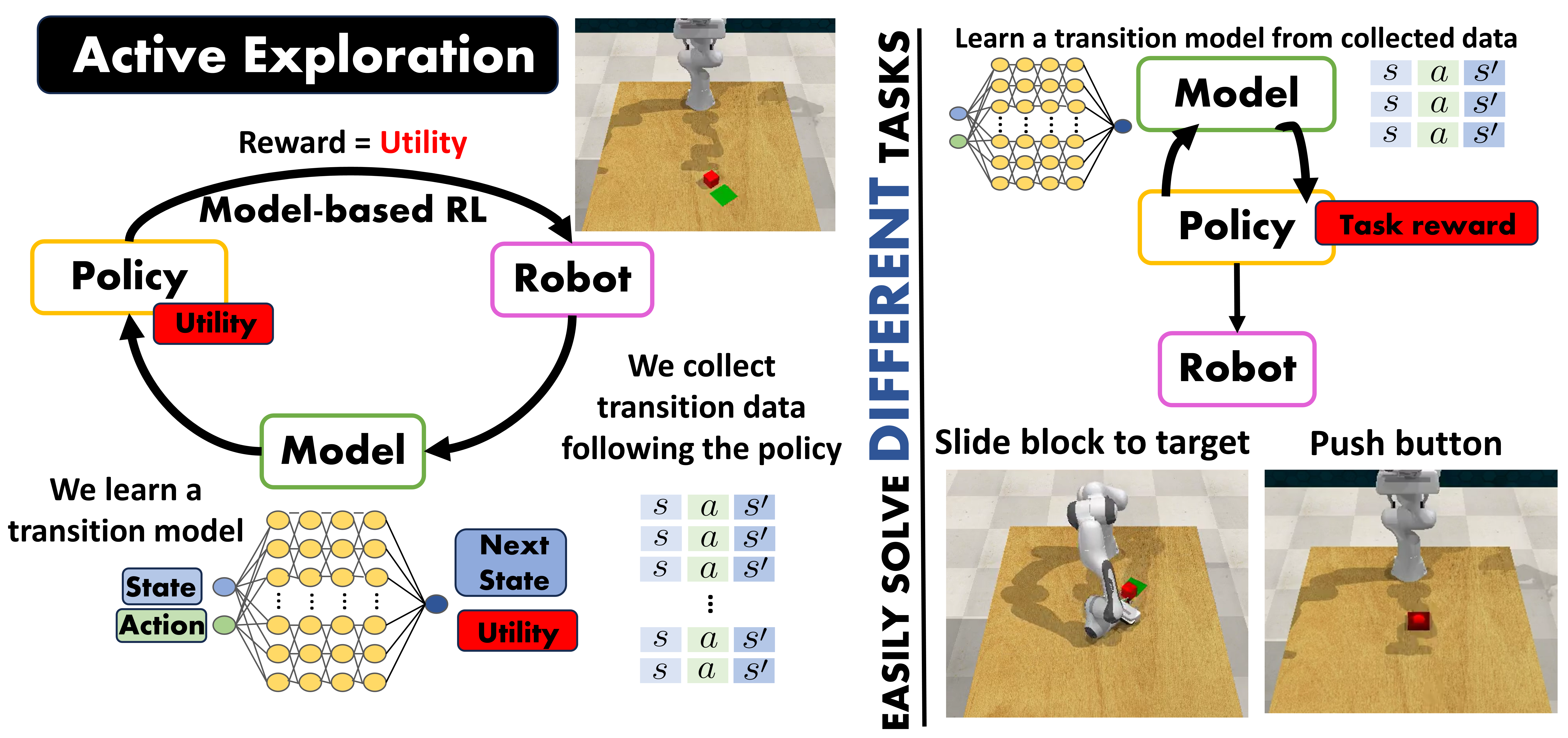
Figure 1: Overview of the active exploration problem through Bayesian model-based RL. The Bayesian model is responsible for predicting both the next state distribution and its degree of novelty. Lastly, we exploit the knowledge acquired during exploration to solve different tasks.
RL strategies are grouped in two main branches: (1) model-based approaches in which the policy is built from simulated episodes, using a model that has been previously learnt to emulate the dynamics of the robot and the environment -i.e., to predict the resulting state after taking an action from the current state- and (2) model-free strategies in which the policy is directly built from episode execution in the robotic platform.
Model-based RL (MBRL) approaches are more sample efficient than model-free strategies since they utilize a model of the environment, akin to human imagination, to predict the outcomes of various actions. By leveraging this predictive capability, MBRL can select appropriate actions without the need for extensive trial and error in the real robot, thereby reducing the associated costs in terms of sample requirements [8]. Furthermore, if we get a model that emulates the robot dynamics, we can leverage it to solve as many tasks as wanted, efficiently building a specific policy for each task.
To develop a model capable of simulating dynamics, it is essential to gather comprehensive data that accurately reflects these dynamics. This data collection is crucial for the model’s training and, consequently, for building useful policies. Active learning appears as a highly suitable tool for this exploration. Active learning states that if a learning algorithm is allowed to choose the data from which it learns, it can yield enhanced performance levels with reduced training requirements. In this work, we leverage active learning basis to guide the exploration towards the most unknown regions of the state space, so as to learn more about them. The main challenge in this setting is to define a reward or utility which measures the information gain of visiting a region, which intrinsically requires a way to capture the information or uncertainty that is captured in a model and the novel observations.
One approach for incorporating uncertainty in deep learning models is Bayesian deep learning (BDL), a branch of deep learning which leverages Bayesian statistics theory and enables to compute the information gain for observing new data. In this paper, we take advantage of BDL techniques to make our model Bayesian and, hence, exploit the uncertainty measure and compute the information utility of the exploration problem. Furthermore, quantifying how certain a deep learning model is about its prediction is essential in a vast amount of deep learning applications as it provides more robust predictions and is fundamental for safety related applications, such as medical applications or human-robot interaction.
To summarise, we propose how to combine some basis of BDL and active learning to efficiently explore the action and state spaces of a RL agent. Unlike other RL strategies that directly construct policies aimed at solving specific tasks, our approach is centered on thoroughly understanding the dynamics of the robot and the environment to, construct tailored policies for solving each of the diverse end-tasks with minimal interaction with the real robot. Our paper undertakes a comprehensive examination of diverse BDL techniques and information-based measures, showcasing superior performance, calibration, and efficiency compared to state-of-the-art methods across multiple environments. Remarkably, our work extends the demonstration to robotic arms, opening new lines of research in this domain. Figure 1 shows an overview of our work, with a specific focus on the robotic arm environment in which it will operate.
2 RELATED WORK↩︎
This work explores novel RL strategies for robotic manipulation using BDL. We next discuss key related works in model-based RL, centering on the exploration, as well as relevant prior work on BDL.
2.1 Model-based Reinforcement Learning↩︎
Among the various RL research directions, MBRL stands out as a promising avenue to enhance the sample efficiency, benefiting a wide range of applications such as trajectory sampling [9] or robot navigation [10]. In MBRL, a model is employed to learn the dynamics of state transitions. Current methodologies for constructing such models encompass both non-parametric such as Gaussian processes [11] or parametric, such as neural networks [12], [13] making either deterministic [14] or probabilistic predictions [15]. An alternative involves world models which leverage generative models to hallucinate its own environment [16], [17]. However, learning an accurate model in diverse DRL tasks with relatively complex environments as robotic manipulation is not a straightforward endeavor. Hence, our emphasis will be on pursuing a thorough exploration of the dynamics to obtain the most accurate model. In addition, MBRL based on Bayesian neural networks use deep ensembles which states to train N models with different architectures, hyperparameters, or initial weights [18]. This is a very effective method [19], [20] but computationally expensive due to the need for training multiple networks. In contrast, MC-dropout approximates the posterior distribution through sampling M forward passes, while maintaining dropout layers active during inference [21], thus requiring training the network only once. In contrast, the Laplace approximation tries to find a Gaussian approximation to the posterior distribution of the weights [22], which has great advantages for robotics applications and provides better calibrations.
2.2 Exploration and Active Learning in DRL↩︎
Most of the exploration algorithms in reinforcement learning are reactive exploration methods. These methods rely on chance discoveries to drive exploration [23], [24]. The agent explores the environment in a more random manner, hoping to accidentally find new and interesting areas. In contrast, a new trend is active exploration which exploits the active learning theory [25].
In the realm of machine learning, active learning (similarly to experimental design in other fields [26]) stands as a prominent strategy that optimizes the learning process by iteratively selecting the most informative instances from an unlabeled dataset [27]. Previous work have addressed exploration for Transition Query Reinforcement Learning where all transitions are available for querying directly [28]. However, in the general case in RL, most transitions are only available once the agent has reached a certain state, forcing to develop full active exploration policies instead of querying methods [26]. Active exploration is more efficient and effective in high-dimensional environments. This approach requires a novelty or information-based measure which existing formulations include visitation count [24], [29], prediction error [30], [31], learning progress [32] and diversity in the visited states [33], [34]. Other approaches leverage deep ensembles technique to compute the utility as either the variance [35] or the Jensen-Rényi Divergence [25] among samples. In contrast, we measure utility leveraging the entropy of the predictive distribution computed by Laplace Approximation.
3 BAYESIAN MODEL-BASED REINFORCEMENT LEARNING↩︎
Let the problem be represented as a Markov decision process (MDP) tuple \((\mathcal{S}, \mathcal{A}, t^*, R, \rho_0)\) where \(\mathcal{S}\) is the state space, \(\mathcal{A}\) is the action space, \(t^* = p_*(s'|s, a): \mathcal{S} \times \mathcal{A} \times \mathcal{S} \rightarrow [0,+\infty)\) is the transition function, possibly unknown, representing the probability of reaching next state \(s'\) given the current state \(s\) and taking action \(a\), \(R: \mathcal{S} \times \mathcal{A} \rightarrow \mathbb{R}\) is the reward function and \(\rho_0\) is the probability density function of the initial state. Without loss of generality, we are going to assume that both state and action spaces \((\mathcal{S}, \mathcal{A})\) are continuous.
In MBRL we build a probabilistic model to predict the distribution of the transition model, that is, \(p_{*}(s'| s, a)\). We will regard this model as a neural network with weights \(\mathbf{\theta}\). This neural network can output the parameters of a Gaussian distribution \((\mu_\mathbf{\theta}, \sigma_\mathbf{\theta})\) so as to predict the probability distribution \(p(s'| s, a, \mathbf{\theta})\). In mathematical terms, \[p (s' | s, a, \mathbf{\theta}) \sim \mathcal{N}(s' | \mu_\mathbf{\theta}(s, a), \sigma_\mathbf{\theta}(s, a)):=\mathcal{N}_\mathbf{\theta}.\]
This model is usually trained from a replay buffer of collected transitions \(\mathcal{D}\) -i.e., sequences of states and actions as inputs \(\{(s_{i}, a_{i})\}_{i=1}^{n}\) and next states as outcomes or labels \(\{s'_{i}\}_{i=1}^{n}\)- to find the maximum a posteriori (MAP) of their weights, \[\label{MAP} \mathbf{\theta}_{MAP} = \mathop{\mathrm{arg\,max}}_{\mathbf{\theta}} \log p(\mathbf{\theta}|\mathcal{D}) = \mathop{\mathrm{arg\,max}}_{\mathbf{\theta}} \log p(\mathcal{D}|\mathbf{\theta})p(\mathbf{\theta}),\tag{1}\] where, first, \(p(\mathcal{D}|\mathbf{\theta})\) is the likelihood and, second, the prior distribution of the weights is \(p(\mathbf{\theta}) \sim \mathcal{N}(0, 1/\gamma^2)\), where \(\gamma^2\) is the prior precision. As result, we get \(\mathcal{N}_{\mathbf{\theta}_{MAP}}\).
However, this strategy lacks proper uncertainty calibration because it captures only the uncertainty associated with the data, called aleatoric uncertainty, but it misses any model uncertainty, called epistemic uncertainty. A more reliable prediction is to compute a distribution over model parameters \(p(\mathbf{\theta}|\mathcal{D})\) and compute the transition function by marginalization of those parameters, that is: \[\label{eq:pred} p(s'| s, a) = \int_\Theta p(s'|s,a, \mathbf{\theta}) p(\mathbf{\theta}|\mathcal{D}) d \mathbf{\theta}.\tag{2}\] By capturing the epistemic uncertainty, we are able to determine how much knowledge a model has and, more importantly for exploration, how much knowledge can be incorporated by adding new data (Figure 2). However, this equation is intractable and we must rely on approximate solutions to estimate it as described next (Figure 3).
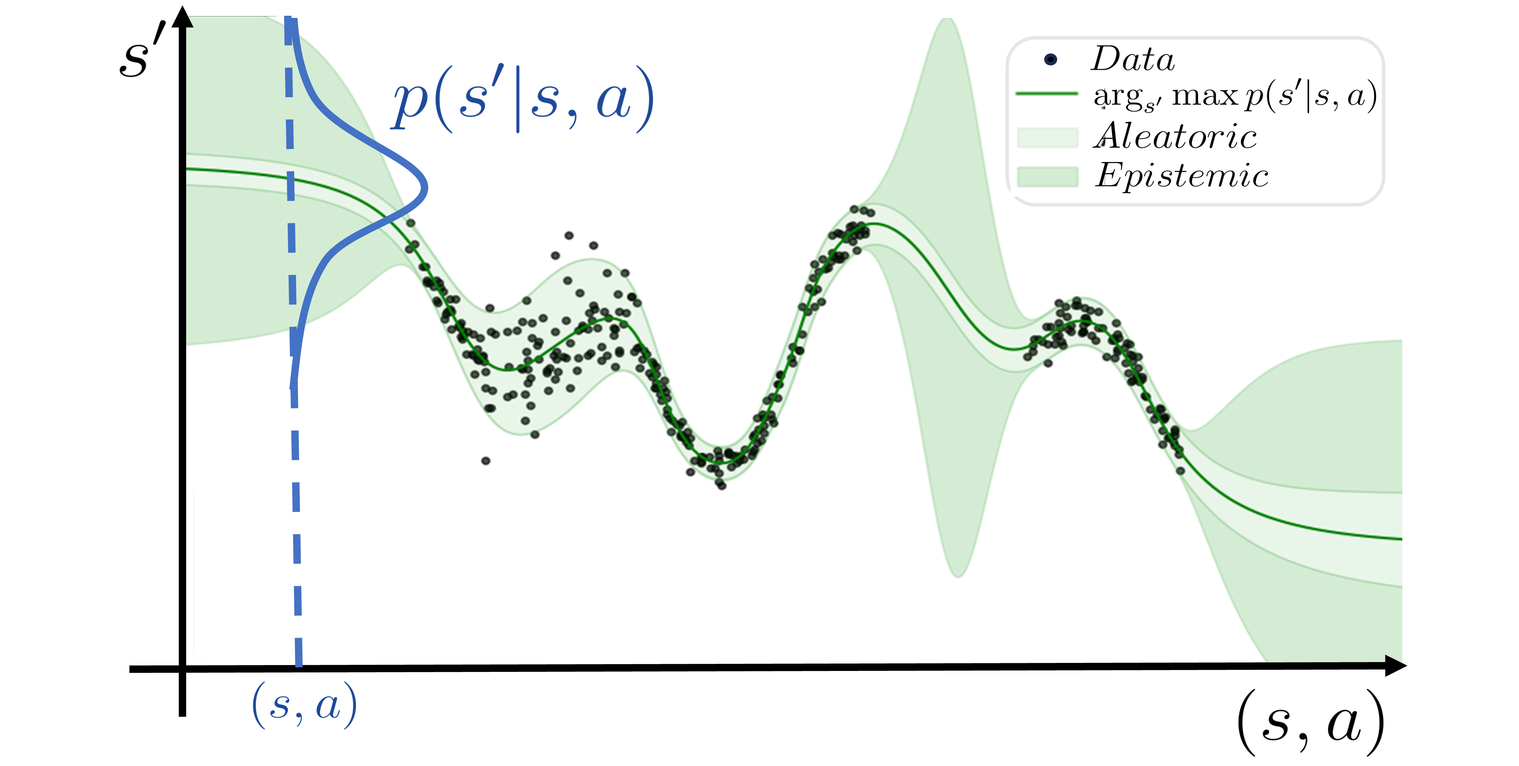
Figure 2: Scheme of our Bayesian model in a toy example. The plot shows the difference between the aleatoric and the epistemic uncertainty. Besides, it showcases the predictive distribution for a given pair \((s, a)\).
3.1 Approximate Bayesian inference↩︎
Previous works that rely on Bayesian deep learning for MBRL use deep ensembles for approximate inference [25], [35]. This method has become popular due to its predictive performance and simplicity to implement, as the Bayesian model is built using several networks trained from random initial parameters. The method is highly expensive both in terms on computing power, as the training process needs to be replicated multiple times, and in memory footprint, as the approach needs to manage and maintain several models at once. Furthermore, as the models need to be trained from random initializations, they cannot be pretrained or fine-tuned, limiting the transfer learning capabilities.
This work studies alternatives to deep ensembles in RL and robotics (Laplace approximation and Monte Carlo dropout) with the following characteristics: computationally efficient, excellent performance and the possibility of using pretrained networks. This makes these alternatives easy to integrate in an existing learning pipeline and aims to overcome the computational constraints associated with the deep ensembles technique.
Deep ensembles-. This method uses Bayesian model average through computing the predictive posterior by marginalization of the model weights \(\mathbf{\theta}\) trained on dataset \(\mathcal{D}\) [18]. Although strictly speaking, the deep ensemble samples are not generated from the full posterior distribution \(p(\mathbf{\theta}| \mathcal{D})\). The fact that they start from random locations may capture the multimodality of the predictive posterior distribution [19]. Hence, following [35] we randomly initialize \(N\) neural networks and train them to find their MAP estimates \(\left\{ \mathbf{\theta}_{1}, \ldots, \mathbf{\theta}_{N}\right\}\). Figure 4 shows an scheme of this method and the alternatives studied, described next.
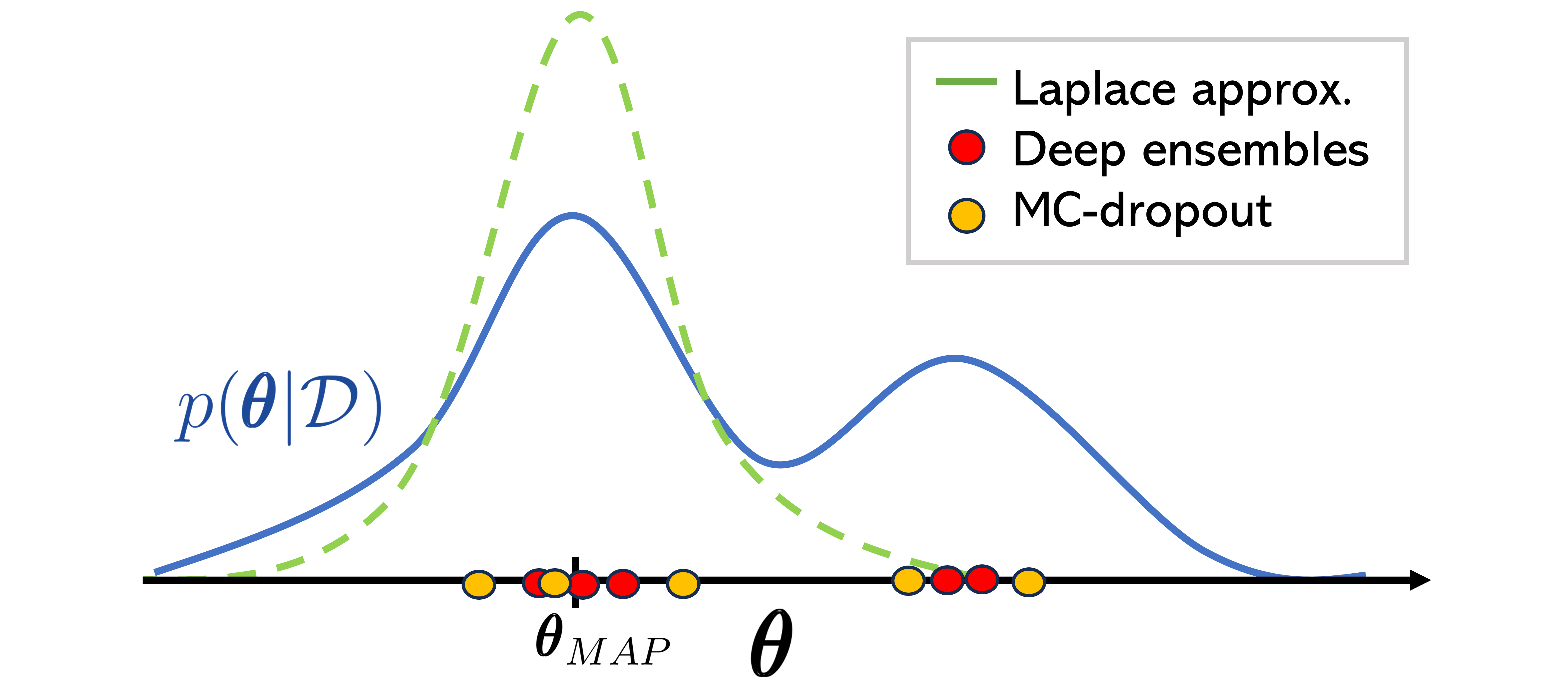
Figure 3: Differences among BDL methods for approximating the posterior distribution \(p(\mathbf{\theta}| \mathcal{D})\). While deep ensembles and MC-dropout both yield sampling approaches around the different local maxima of the posterior, Laplace approach estimates a Gaussian distribution around its peak \(\mathbf{\theta}_{MAP}\).
Monte Carlo dropout-. Monte Carlo dropout (MC-droput) approximates the posterior as the sample distribution of \(N\) forward passes during inference time, maintaining active the random dropout layers. In other words, the network includes some dropout layers which are kept active at inference time.
Laplace approximation-. Trying to cover the predictive distribution 2 in a more reliable way, we may approximate the posterior distribution of the weights through Laplace approximation [22] as a Gaussian distribution, \[\label{eq:LapApp} p(\mathbf{\theta}|\mathcal{D}) \approx \mathcal{N}(\mathbf{\theta}|\mathbf{\theta}_{MAP}, \mathbf{H}^{-1}),\tag{3}\] where \(\mathbf{H}=\nabla^{2}_{\mathbf{\theta}} \log p(\mathcal{D}|\mathbf{\theta})|_{\mathbf{\theta}_{MAP}}\) and, subsequently, translate this uncertainty into the predictive variable. A first-order Taylor approximation (linearization) allows us to get a Gaussian predictive distribution \[\label{eq:PredLap} p(s'| s, a) \approx \mathcal{N}(s' | \mu_{\mathbf{\theta}_{MAP}}, \mathbf{J}^{T}\mathbf{H}^{-1}\mathbf{J} + \text{diag}(\sigma_{\mathbf{\theta}_{MAP}})),\tag{4}\] where \([\mu_{\mathbf{\theta}_{MAP}},\sigma_{\mathbf{\theta}_{MAP}}] = f_{\mathbf{\theta}_{MAP}}(s,a)\) is the network prediction and \(\mathbf{J}=\nabla_{\mathbf{\theta}}\mu_{\mathbf{\theta}}(s, a)|_{\mathbf{\theta}_{MAP}}\). Nevertheless, when dealing with larger models, we are obliged to apply subnetwork inference. This technique considers as Bayesian weights only the \(n_{sub}\) weights with greatest absolute values; i.e, the \(n_{sub}\) weights that are theoretically more relevant [36]. Besides, to translate this uncertainty into the predictive distribution, we will leverage Monte Carlo. Specifically, we take \(N\) samples of the subnetwork weights from 3 and perform a forward pass per sample, setting the remaining weights with their MAP estimate value.
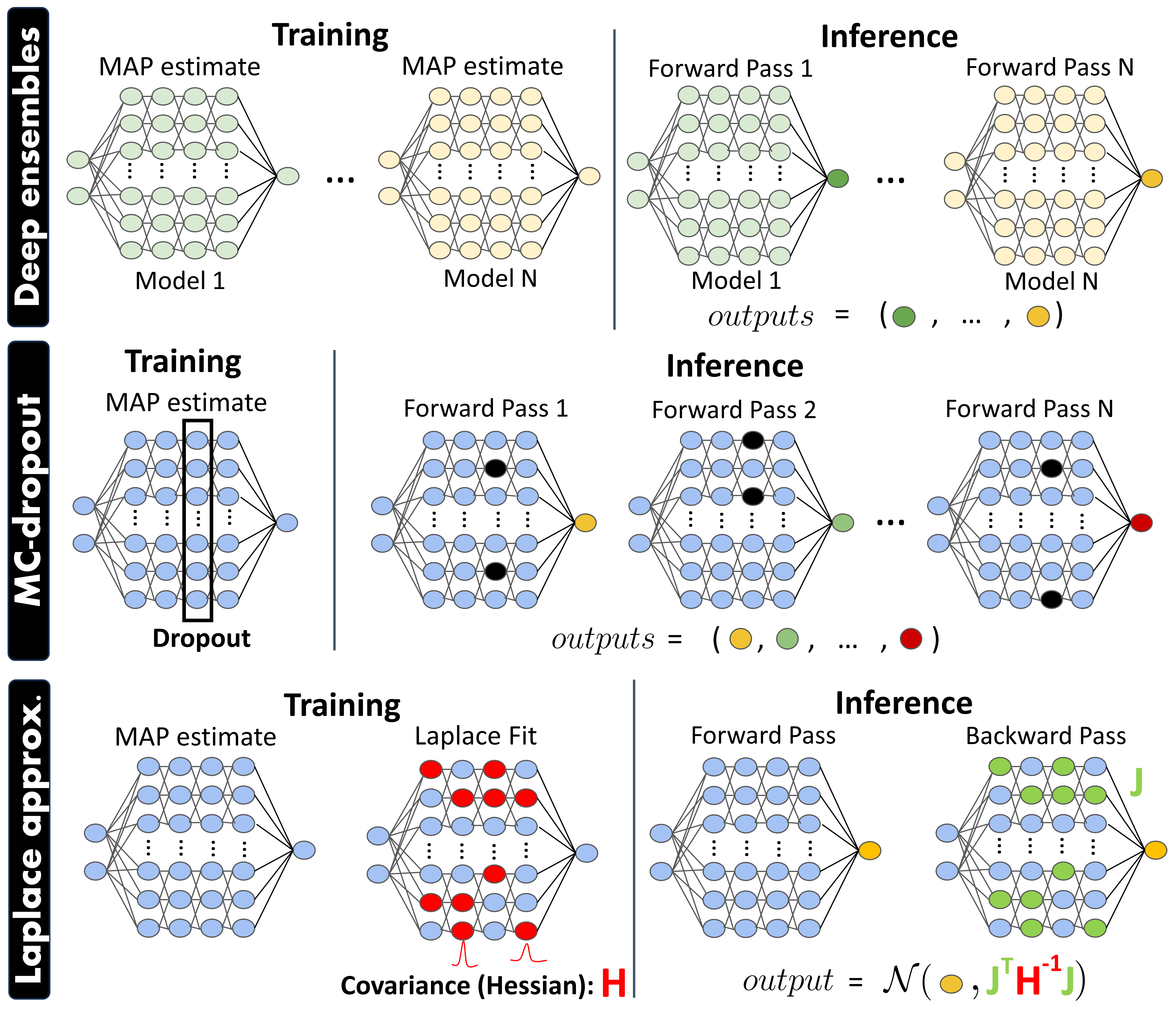
Figure 4: Scheme of BDL methods for approximating the predictive distribution in a neural network. While deep ensembles and MC-dropout get samples from multiple forward passes, Laplace method estimates a Gaussian through linearization technique (in the picture, the Laplace method is applied in a subnetwork).
4 EXPLORATION FOR MBRL↩︎
In the context of this work, we define the exploration problem as gathering valuable information in the replay buffer \(\mathcal{D}\) to learn the most accurate dynamic model \(p(s'|s,a)\). Therefore, we can pose the exploration problem as an active learning problem. However, contrary to pure query strategy [28], data cannot be queried independently since a given state can only be reached by querying a previous sequence of states and actions that reaches the target state. Thus, our exploration problem can be defined as a MDP \((\mathcal{S}, \mathcal{A}, t^*, u, \rho_0)\), similar to the one presented in Section 3, replacing the reward task by a utility function \(u\) that measures the novelty of the transition.
4.1 Exploration as experimental design↩︎
In our framework, we set an exploration MDP where the reward term is an experimental desing based utility. This utility is based on the expected information gain (IG) obtained by reaching and observing future state-action pair \((s,a)\). The information gain may be defined as the amount of information gained about a random variable or signal from observing another random variable. In our scenario, the information gain by a transition \(z = \{s, a, s'\}\) can be defined as the KL-divergence of the model posterior distribution after and before adding the transition data, that is: \[\label{eq:IG} IG(s, a, s') = D_{KL}\left(p(\mathbf{\theta}|\mathcal{D}\cup z) \;\Vert\; p(\mathbf{\theta}|\mathcal{D})\right),\tag{5}\] From this expression, the utility of an action is: \[\label{eq:Utility} u(s, a) = \int_{\mathcal{S}}IG(s, a, s')p(s'|s, a) ds',\tag{6}\] which can be used to compute the utility of a policy \[U(\pi) = \mathbb{E}_{p(\mathbf{\theta}|\mathcal{D})}\left[\mathbb{E}_{p(s,a|\pi,\mathbf{\theta})}[u(s, a]\right]\] where \(p(s,a|\pi,\mathbf{\theta})\) is the probability of being in state \(s\) and selecting action \(a\) by following the policy \(\pi\) and the transition model defined by \(\mathbf{\theta}\). Then, we can also define the action utility as the Jensen-Shanon (JS) divergence following the derivation of Shyam et al. [25]: \[u(s, a) = \mathcal{H}_{s'} \left(\mathbb{E}_{\mathbf{\theta}}\left[p(s'|s, a, \mathbf{\theta})\right]\right) - \mathbb{E}_{\mathbf{\theta}} \left[\mathcal{H}_{s'} \left( p(s'|s, a, \mathbf{\theta}) \right)\right]\] note that the first term corresponds to the entropy of \(\mathbb{E}_{\mathbf{\theta}}\left[p(s'|s, a, \mathbf{\theta})\right]\), which is exactly the predictive posterior as defined in equation 2 . Conceptually, it captures the total uncertainty (epistemic and aleatoric) of our model. The second term represents the expected entropy of the predictive distribution, that is, the aleatoric uncertainty. Therefore, we can see how the JS divergence is maximized where the epistemic uncertainty is maximized. This is consistent with the classical interpretation of epistemic uncertainty which captures the information or knowledge encoded in the model, contrary to the aleatoric uncertainty which encodes the data noise. Intuitively, the exploration is driven by data where we have high uncertainty because our model lacks information, not because the data themselves are noisy.
If we have a sample representation of our model \(\{\mathbf{\theta}_i\}_{i=1}^N\), like in the case of deep ensembles of MC-dropout, we can compute the utility as the utility of a mixture of Gaussians: \[\label{eq:js95sample} u(s, a) = \mathcal{H}\left(\frac{1}{N}\sum_{i=1}^{N}\mathcal{N}_{\mathbf{\theta}_{i}} \right) -\frac{1}{N}\sum_{i=1}^{N} \mathcal{H}\left( \mathcal{N}_{\mathbf{\theta}_{i}} \right).\tag{7}\] However, the first term is the Shanon entropy of a mixture of Gaussians which does not have analytical solution. Instead, we can use the generalized Rényi entropy \(\mathcal{H}_\alpha\) with \(\alpha=2\) which has a closed form [25]. Note that the Shanon entropy is \(\mathcal{H} = \lim_{\alpha \rightarrow 1} \mathcal{H}_\alpha\). The problem of Rényi entropy with \(\alpha > 1\) is that it is biased towards events of higher probability and ignores events of low probability.
One advantage of the Laplace approximation is that the posterior model is approximated as a Gaussian distribution with a predictive covariance \(\Sigma_{LA} = \mathbf{J}^{T}\mathbf{H}^{-1}\mathbf{J} + \sigma_{\mathbf{\theta}_{MAP}}(s, a))\). Thus, \[\begin{align} \label{eq:js95gaussian} \mathcal{H}_{s'} \left(\mathbb{E}_{\mathbf{\theta}}\left[p(s'|s, a, \mathbf{\theta})\right]\right) &\stackrel{c}{=} -\log|\Sigma_{LA}|\\ \mathbb{E}_{\mathbf{\theta}} \left[\mathcal{H}_{s'} \left( p(s'|s, a, \mathbf{\theta}) \right)\right] &\stackrel{c}{=} -\mathbb{E}_{\mathbf{\theta}} \left[\log|\sigma_{\mathbf{\theta}}(s, a))|\right] \end{align}\tag{8}\] where \(\stackrel{c}{=}\) represents equal up to a constant term. In general, the second term does not have analytical form. However, we can assume homoscedastic noise, that is, \(\sigma_\mathbf{\theta}\) is a constant value, independent of \((s, a)\). In practice, we found that even if we try to learn heteroscedastic noise dependent of the current state and action, the variability is negligible compared to other terms. Therefore, if we assume homoscedastic noise, we can simplify our utility function: \[u(s,a) \stackrel{c}{=} \mathcal{H}_{s'} \left(\mathbb{E}_{\mathbf{\theta}}\left[p(s'|s, a, \mathbf{\theta})\right]\right) \stackrel{c}{=} -\log|\mathbf{J}^{T}\mathbf{H}^{-1}\mathbf{J}|.\] This metric, which we call directly entropy metric, can be seen as a particular case of the idea commented before that epistemic uncertainty has to be the driving factor in exploration. This metric is also related to other metrics based on disagreement [35]. In fact, we can also define a metric based purely on the entropy of the predictive model using the sample approximation of MC-dropout or deep ensembles.
Starting from 7 , instead of approximating by Rényi entropy, we can approximate the mixture of Gaussians \(\left\{\mathcal{N}_{\mathbf{\theta}_{1}}, \ldots, \mathcal{N}_{\mathbf{\theta}_{N}} \right\}\) by a new Gaussian \(\mathcal{N}_{M}\) with mean \(\mathbf{\mu}_{M} = \frac{1}{N}\sum_{i=1}^{N} \mu_{\mathbf{\theta}_i}\) and covariance \(\Sigma_{M}\) defined as, \[\Sigma_{M} = \frac{1}{N} \sum_{i=1}^{N} \left( \text{diag}(\sigma_{\mathbf{\theta}_i}) + \mu_{\mathbf{\theta}_i}\mu_{\mathbf{\theta}_i}^T \right) - \mu_{M}\mu_{M}^T\] Then, if we also assume homoscedastic noise, we get a the entropy metric based on samples: \[u(s,a) \stackrel{c}{=} -\log \left| \frac{1}{N} \sum_{i=1}^{N} \mu_{\mathbf{\theta}_i}\mu_{\mathbf{\theta}_i}^T - \mu_{M}\mu_{M}^T \right|.\]
5 PIPELINE↩︎
The pipeline followed to explore and evaluate is inspired by Shyam et al. [25]. This section describes our pipeline main stages, which are summarized in Figure 5.

Figure 5: Summary of both exploration and evaluation pipelines with their key stages. The starting points are marked with Init. Particularly, the exploration begins collecting data from a random policy and the evaluation starts from the buffer of trajectories collected along the exploration.
5.1 Exploration Pipeline↩︎
First of all, the backbone and focus of this problem is the exploration algorithm. This may be summarized as follows:
The agent starts acting randomly along \(n^{ex}_{warm}\) steps. As our agent interacts with the environment, it collects trajectories of the form \(\{s_{i}, a_{i}, s_{i}'\}\) in the buffer \(\mathcal{D}\), where \(i\) denotes the number of exploration steps.
We train a model \(f^{ex}\) from \(\mathcal{D}\) that learns to simulate the dynamics of the robot. We leverage this model to build an exploration policy \(\pi^{ex}\) which uses the information gain measure as utility.
The agent acts along \(n_{pol}\) steps following policy \(\pi^{ex}\). We continue saving these steps \(\{s_{i}, a_{i}, s_{i}'\}\) in \(\mathcal{D}\).
We repeat stages 2-3 until the agent reaches \(n^{ex}_{steps}\) exploration steps. Meanwhile, each \(n_{eval}\) exploration steps, we evaluate the exploration accomplished up to that moment, entering in the evaluation pipeline with all the collected trajectories \(\mathcal{D}\) up to that moment.
5.2 Evaluation Pipeline↩︎
We will enter in this pipeline to evalute the exploration conducted. To achieve this goal, we will try to solve a task from the knowledge attained in the exploration pipeline. Theoretically, the more exhaustive the exploration, the better the performance trying to solve the task. Hence, the evaluation pipeline may be explained in the next steps:
For each task of the environment, we repeat \(n_{k}\) times the following stages in order to get a more accurate estimate of the agent’s performance.
We train a model \(f^{ev}\) with all the collected trajectories \(\mathcal{D}\) up to that moment to simulate the dynamics of the robot. We use this model to rapidly build an evaluation policy \(\pi^{ev}\) following the reward of the desired task.
The agent acts along \(n^{ev}_{steps}\) steps following policy \(\pi^{ev}\). The evaluation metric is either the sum or the maximum of the task reward along these steps.
For learning both pure exploration and task-specific policies from the model, we employed Soft-Actor Critic (SAC) which is the gold standard for reinforcement learning in robotics [37]. Specifically, we run \(n^{pol}_{eps}\) episodes along \(n^{pol}_{steps}\) steps, during which the trained model \(f\) forecasts the consequences of the taken actions.
This algorithm offers a significant efficiency advantage over model-free approaches, particularly in the total number of steps performed by the robot. For instance, employing SAC directly without a model would require \(n_{t}\cdot n_{k} \cdot n^{SAC}_{steps}\) real world interactions, where \(n_{t}\) denotes the number of tasks. In contrast, with this pipeline, the robot only needs to execute \(n^{ex}_{steps}\), which is substantially fewer than \(n^{SAC}_{steps}\), as we will observe in Section6. This difference arises because the model is responsible for simulating most of the steps, demonstrating an improvement in sampling efficiency.
6 Evaluation details↩︎
6.1 Environments↩︎
In order to evaluate our approach to model-based active exploration, we conducted experiments on several continuous environments of two widely used benchmarks such as OpenAI Gym [38] and RLBench [39]. First, the tasks of OpenAI Gym are built using the MuJoCo physics engine [40]. These are some commonly used environments in the RL literature, and consequently, we will utilize them for comparison with other studies. Second, RLBench is built around a CoppeliaSim/V-REP [41]. We also test our Bayesian approaches and information metrics in a realistic robot manipulation problem, increasing the task’s difficulty and consequently amplifying the challenge for the exploration algorithm. Specifically, the environments and tasks are the following ones:
HalfCheetah-. It is a MuJoCo based planar kinematic string whose state space (\(|\mathcal{S}|=17\)) consists of the positional and velocity values of different joints, while the action space contains 6 continuous torques applied to the robot’s joints. In this problem we considered two different tasks: (1) Running: move forward as faster as possible and (2) Flipping: perform flips.Coppelia-. We utilize the Panda robot, with a state space (\(|\mathcal{S}|=43\)) encompassing the position, velocity, and forces of both its joints and gripper. Moreover, its action space comprises \(8\) velocity joints. We employed two different RlBench tasks: (1) PushButton: approximating its grip towards a button and (2) MoveBlockToTarget: push a red block positioned stochastically on a table towards the goal. Both rewards have been redefined to be continuous, ranging from 0 to 100.
6.2 Experimental details↩︎
The base neural network consists of a multi-layer perceptron (MLP) with \(5\) layers and \(512\) neurons per hidden layer. The input and the output sizes of the the MLP are \(|\mathcal{S}|+|\mathcal{A}|\) and \(2|\mathcal{S}|\), respectively. We build the Bayesian approaches taking \(N=32\) models/forward passes/samples. Specifically, dropout is introduced in the middle hidden layer with a probability of \(p=0.25\) and Laplace approximation is applied only in the subnetwork comprised of the \(n_{subnet}=1k\) weights with highest absolute values. Regarding the utility measure, we will compare our entropy measure with respect to the Jensen-Rényi divergence [25].
Concerning the pipeline, we run \(n^{ex}_{steps}=20k\) exploration steps. From which the first \(n^{ex}_{warm}=256\) steps correspond to warm-up. Besides, we recompute the exploration policy each \(n_{pol}=25\) exploration steps and evaluate each \(n_{eval}=2000\) exploration steps. First, to compute the exploration policy, we run \(n^{pol}_{eps}=50\) episodes along \(n^{pol}_{steps}=50\) steps where the consequence of \(n_{act}=128\) actions are computed simultaneously. Second, to evaluate the specific task we run \(n_k=3\) evaluation episodes in which we start computing the task policy (\(n^{pol}_{eps}=250, \; n^{pol}_{steps}=100, \; n_{act}=128\)) and, afterwards, we run \(n^{ev}_{steps}=100\) steps.
The experiments were conducted with a Intel Core™ i7-12700K processor with 20 cores, and NVIDIA GeForce RTX 3090 GPU.
7 RESULTS↩︎
In this section, we conduct a comparative analysis of the diverse Bayesian models and utility measures under examination. In addition to reward comparisons, we delve into computational time and storage analyses for the various Bayesian models. The state-of-the-art works selected as baselines can be categorized into three distinct approaches to tackling the challenge:
Model-free RL: Utilizing SAC [37] which is the gold standard algorithm in model-free RL. We construct a policy for each task by executing the same steps on the robotic platform as our exploration process. Besides, we set an upper bound on performance by running SAC for a significantly greater number of steps.
Model-based Exploration: while maintaining the existing pipeline, we replace our exploration approach by a reactive exploration algorithm as PERX [30] and simple naive random exploration.
Model-based active Exploration (MAX) [25]: this work calculates the Jensen-Rényi divergence with a 32-deep ensemble based on equation 7 .
7.1 Rewards↩︎
Our focus is on evaluating the performance of our approaches and baselines concerning exploration. We quantify performance by examining the rewards achieved during the evaluation phase, understanding that a higher task reward corresponds to a more comprehensive understanding of the environment -i.e., indicative of effective exploration-. To ensure a fair comparison, we employ the same Bayesian model in the evaluation stage, uniquely varying the buffer (collected along the exploration) used for model training.
HalfCheetah-. Figure 6 shows how Bayesian model-based active exploration approaches clearly outperform the remaining methods. Specifically, those approaches where the Bayesian model is built from Laplace approximation and MC-dropout (ours) achieve a higher performance than those built from deep ensembles. Furthermore, these results indicate that our utility measure is more suitable for Laplace-based model, whereas deep ensembles fit better with Rényi entropy. Lastly, note that LapMCEnt approach overtakes the performance achieved by SAC despite of running x20 times more steps in the robot (20k vs 2\(\times\)200k).
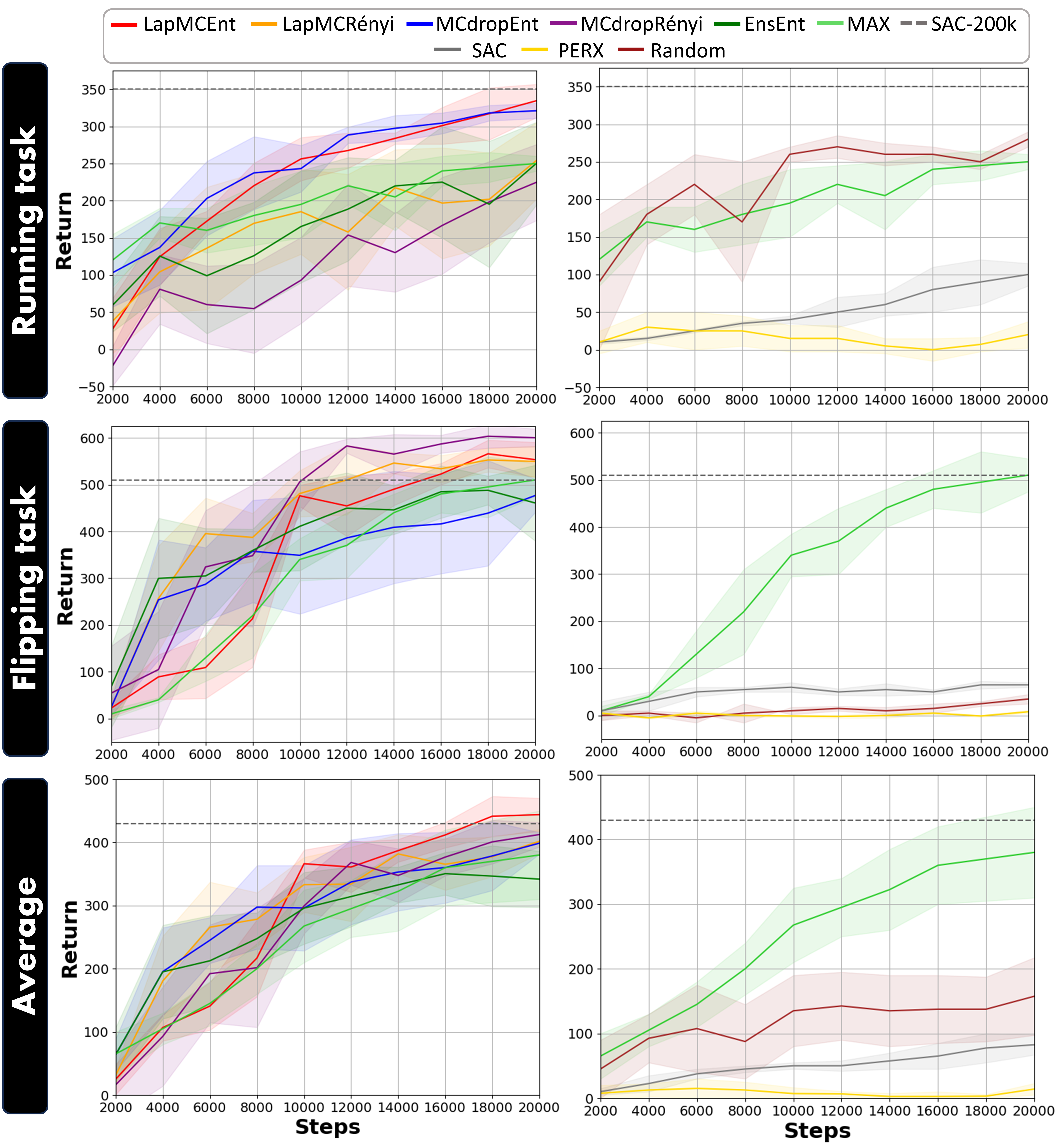
Figure 6: Results in HalfCheetah. First column model-based active exploration algorithms (ours + MAX). Second column, other approaches as presented in [25]. MAX and SAC trained for 200k steps are represented in both sides for reference. As can be seen both Laplace and MC-dropout outperform deep ensembles (MAX and EnsEnt) and the entropy metric is more consistent than the
Jensen-Rényi divergence with Laplace approximation.
Coppelia-. Leveraging the methods that have shown the best performance in HalfCheetah, we focus on our problem of interest: Coppelia. In this high-dimensional environment, we observe again how Bayesian
model-based active exploration approaches outperform the other approaches. These Bayesian approaches achieve a really similar performance. Besides, it is observed the difference in the task complexity. While these methods solve the PushButton task
in nearly all the evaluation episodes, they have some difficulties with MoveBlock task. The reason is that, to solve this task, it is needed to know the dynamics of the box and to get this, the model requires many data about it. Otherwise, it will
predict that the box is never moved. However, this data must be collected by querying a large sequence of states and actions that, finally, ends with an interaction robot-box. Therefore, the data collected along the exploration about the box dynamics does
not seem to be enough for learning its kinetics. Particularly, the peak in the average of both tasks is reached by LapMCEnt.
7.2 Calibration↩︎
From here on, our experiments focus on the HalfCheetah environment to study other interesting metrics. We have observed the significant role of uncertainty estimation in Bayesian models in guiding exploration towards less-explored regions.
It is crucial that this uncertainty aligns with the model’s lack of knowledge (error), i.e., it is well calibrated. To assess this alignment, we utilize the Area Under Sparsification Error curve (AUSE) metric [19]. Specifically, we will leverage the buffer stored at the end of the exploration (20k steps) to train each Bayesian model with the first 18k
steps and test with the last 2k steps. Thus, we will compare its model prediction errors with respect to their utility values. These results can be found in Table 1. Notably, Laplace-based model exhibit the highest calibration performance. MC-dropout and deep ensembles together with Rényi entropy (MAX) trail further in terms of calibration effectiveness.
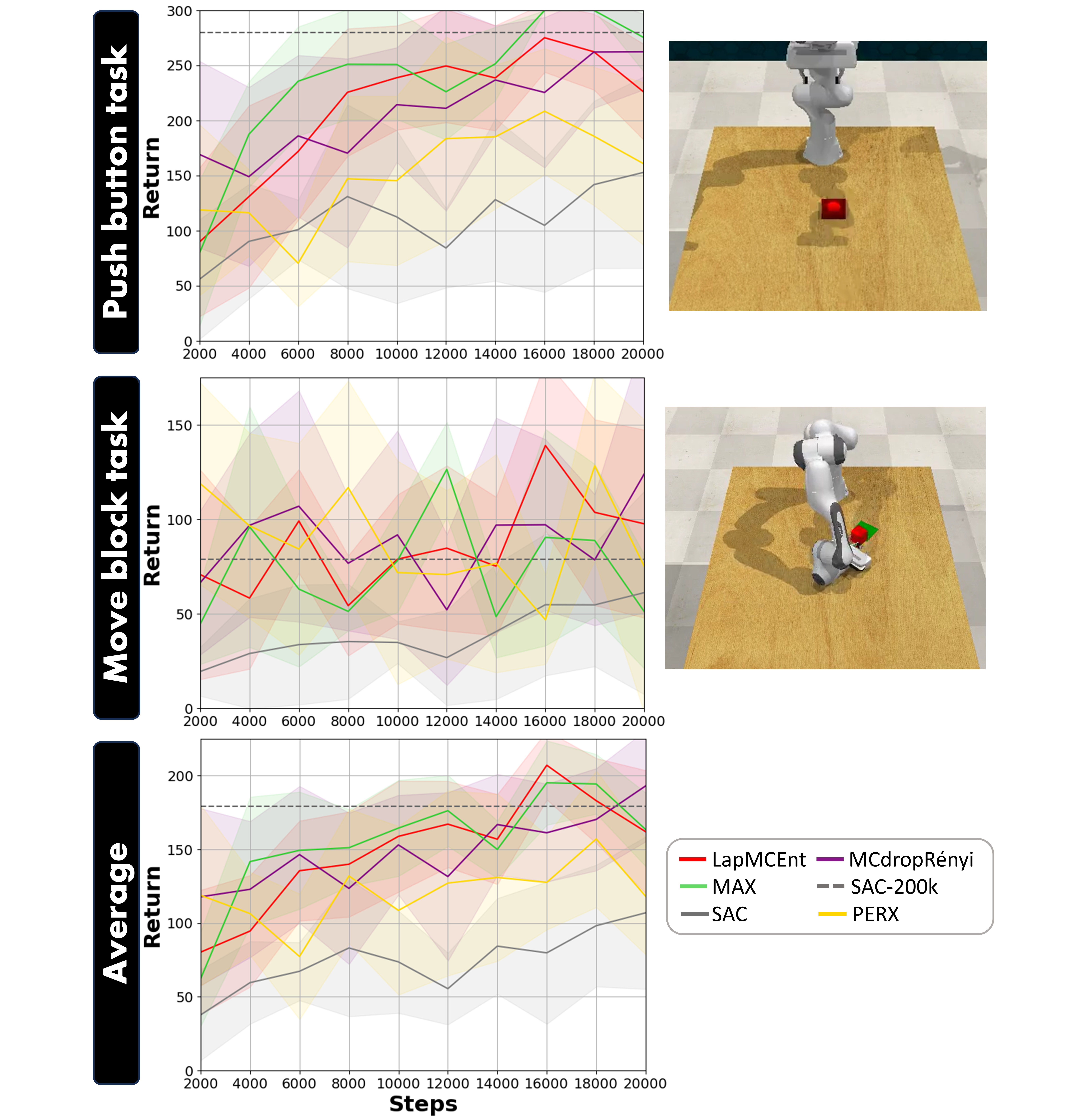
Figure 7: Results in Coppelia for the best approaches. As can be seen, the Laplace approximation with our entropy metric is more robust in the more difficult tasks (move block) due to its better support while sampling methods
overfit to straightforward tasks (push button).
| Model | AUSE \(\downarrow\) | Training (s) | Inference (s) \(\downarrow\) |
|---|---|---|---|
| MAX [25] | 0.075 | 122.75 | 6.25e-3 |
| LapMCEnt | 0.048 | 39.98 | 6.00e-3 |
| MCdropRényi | 0.085 | 34.35 | 6.91e-3 |
7.3 Computational time and load↩︎
Table 1 also includes a comparative assessment of the Bayesian models in terms of computational time and memory efficiency. First, we trained all models with identical training sets (18k buffer size) and measure the time spent in a forward pass (inference).
Remarkably, implementing MAX leads to an increase of training time since it requires to fit \(n_{ens}\) neural networks. Additionally, it is observed that Laplace Approximation introduces extra computational overhead compared to MC-dropout, since it must fit the covariance matrix of the posterior distribution 3 . Regarding inference times, there are no substantial distinctions among Bayesian models.
Finally, we evaluate the Bayesian models from the perspective of storage requirements. The storage demands of these models depend on several factors, including the number of weights (\(n_{weights}\)) in the model, the amount of neural networks (\(n_{ens}\)) stacked to construct deep ensembles, and the size of the covariance matrix for the Laplace Approximation distribution (\(n_{subnet}^{2}\)). We can express the storage cost as, \[Cost = \mathcal{O}\left(n_{ens} \cdot n_{weights} + n_{subnet}^{2}\right).\] In our scenario, wherein our MLP encompasses approximately \(n_{weights} \approx 1M\) of weights, opting for deep emsembles (MAX) leads to a memory overhead 32 times greater than that of MC-dropout and 16 times greater than that of Laplace Approximation, respectively.
8 CONCLUSIONS↩︎
This work demonstrates the benefits of model based RL for robotics systems, where sample efficiency is of paramount importance, by replacing expensive real world interactions by cheap model evaluations during policy training. Furthermore, we can perform active learning on the model reducing even further the need for real world interactions by carefully selecting the most informative ones. In addition, once the model is trained, it can be used for generalization of multiple tasks. The proposed Bayesian models not only pave the way for novel utility formulations but also offer enhancements in performance, calibration, and efficiency. Our research opens avenues for further exploration and application of Bayesian methodologies in addressing complex challenges in RL, such as robotic systems. We also highlight the potential of alternative Bayesian inference methods such as Laplace approximation or MC-dropout which have been barely investigated for robotics applications. In particular, the Laplace approximation presents interesting properties for robotic applications, such as open the posibility of using pretrained or foundational models or having a Gaussian posterior distribution with full support which can be used in posterior decision making.