1 Introduction↩︎

The standard \(\Lambda\)CDMcosmological model, incorporating a cosmological constant, \(\Lambda\), and cold dark matter (DM), has been remarkably successful in interpreting and predicting fundamental properties of the large-scale structure of the Universe. Despite potential tensions [1], [2], this success extends to temperature anisotropies of the cosmic microwave background (CMB), clustering of the distribution of galaxies, and deviations of galaxy motions from a purely Hubble flow [3]–[8]. On galactic scales, predicting the properties of the galaxy population and its evolution with redshift has been less straightforward. This complexity arises from the intricate nature of baryonic physics involved in star formation processes, including gas dynamics, heating and cooling mechanisms, and notably, the energetic feedback from supernovae (SN) and active galactic nuclei (AGNs) [9]–[15].

Prior to the era of the James Webb Space Telescope (JWST) [16], significant efforts have been invested in developing models of galaxy formation to adequately describe observations at low and moderately high redshifts (\(z~\rlap{<}{\lower 1.0ex\sim}10\)) [17].

Observations obtained with the JWST have significantly deepened our view of the universe, revealing galaxies as far back as a couple of hundred million years near the Big Bang. However, the JWST has also detected an unexpected excess of luminous galaxies at higher redshifts. While the initial findings from the JWST appeared to pose serious challenges for the standard \(\Lambda\)CDM model of structure formation, the severity of these discrepancies were significantly alleviated with more precise calibration and the availability of spectroscopic redshifts [18].

It should be emphasized that the star formation rates (SFRs) in high-redshift JWST galaxies are not particularly unusual in themselves [19], [20]. These galaxies exhibit SFRs that can be adequately sustained by cosmological gas accretion onto halos [21]. Matching the abundance of halos to the observed distribution of UV magnitudes (used as proxies for the SFRs) of galaxies at \(z\mathrel{\rlap{\lower 4pt\hskip 0.5pt\sim} \raise 1pt>}10\) implies that these galaxies should be hosted in halos of mass \(M_\textrm{h}\approx 5\times 10^{10}-10^{11}\, {\rm M}_\odot\) [21]–[23]. For such halos, the star formation efficiency \(f_\textrm{SF}\) (i.e. the fraction of accreting gas turning into stars) needed to account for the SFRs, is \(\gtrsim 0.13\) (see 3.2.1 below). At low redshifts (\(z\lesssim 4\)), the stellar-to-halo mass ratio (SHMR) inferred from abundance matching is in the range \(0.001-0.01\) for \(M_\textrm{h}\approx 10^{11}\, {\rm M}_\odot\) halos [24]–[27]. Assuming a global gas fraction \(f_\textrm{b}=0.157\) in galaxies [7], this implies an average star formation efficiency, \(f_\textrm{SF}\approx 0.06 -0.006\), which is at least a factor of two lower than the inferred value at \(z\gtrsim 10\).

An important aspect of star formation inside DM halos is their mass accretion history [11]. Halo accretion is directly linked to the availability of gas for star formation. Newly accreted gas replenishes the reservoir, which is subsequently converted into stars and may escape the galaxy through processes like SN and AGN feedback. In this paper, we assume that \(z\gtrsim 10\) galaxies indeed inhabit massive halos and aim to numerically investigate the assembly history of these halos. Numerical studies of individual objects typically rely on the methodology of zoom-in simulations [28]–[31]. In this type of simulations high resolution is employed only in a small region allowing a detailed study of its small scale dynamics while simultaneously capturing the interaction within the larger cosmic environment. In this paper we invoke an alternative approach of constrained simulations [32] to model the high redshift \(z>9\) accretion history of halos above \(M_\textrm{h}\approx 10^{11} \, {\rm M}_\odot\). We utilize the [33] method of constrained random realizations to generate initial conditions that are guaranteed to contain a halo in specified mass range, when evolved forward to a specified redshift, \(z\).

The technique of constrained simulations is very useful in large scale structure studies, especially for assessing uncertainties in parameter estimations realistically and in mitigating cosmic variance [34]. This approach has been used to derive simulation initial conditions from the observed peculiar velocities [35] and from the 2MRS redshift survey [8]. Initial conditions based on the galaxy distribution in the Sloan Digital Sky Survey (SDSS) survey have also been generated to run a constrained simulation to study the local Universe [36]. The same simulation has also been utilised to study the \(z\simeq 0\) descendants of galaxies at \(z\approx 8-9\) galaxies [23].

The structure of the paper is outlined as follows. In §2, we assess the abundance of halos and compare is with the luminosity function of galaxies at high redshifts. We underscore the advantage of constrained simulations based on the expected abundance of the host halos. The simulations are detailed in §3, which includes the method for generating suitable initial conditions. Additionally, this section contrasts the accretion history of halos in the simulations with observational data. In §4, a straightforward recipe for star formation is introduced. The recipes produces a higher ratio of stellar to halo mass at high redshifts compared to low redshift. A summary and discussion are provided in §5.

We adopt the standard flat \(\Lambda\)CDMcosmological model [7] with a total mass density parameter \(\Omega_m=0.311\), baryonic density \(\Omega_b=0.049\), Hubble constant \(H_0=67.7\, {\rm km }\, {\rm s}^{-1}\, \, \rm Mpc^{-1}\) and normalization \(\sigma_8=0.81\).

2 Halo abundance at high redshift↩︎

We employ a halo definition in terms of a spherical overdensity, where the halo virial radius \(r_\textrm{h}(t)\), at any given time \(t\) is determined such that the mean density within this radius equals \(200\) times the critical density of the universe, \(\rho_c(t)= 3H(t)^2/8\pi G\). Therefore, \[\begin{align} \label{eq:vir} r_\textrm{h}(t) & = 0.1 H(t)^{-1}V_c \; , \nonumber \\ M_\textrm{h}(t) & = 0.1 G^{-1} H(t)^{-1} V_c^3 \; , \end{align}\tag{1}\] where the circular velocity \(V_\textrm{c}=\sqrt{G M_\textrm{h}/r_\textrm{h}}\). At high redshifts where \(H\sim 1/t\), these relations yield \[\begin{align} \label{eq:virN} r_\textrm{h}(t) & = 13.1\, {\rm kpc }\left(\frac{11}{1+z}\right)^{3/2}\frac{V_c}{181\, {\rm km }\, {\rm s}^{-1}} \; , \nonumber \\ M_\textrm{h}(t) & = 10^{11}\, {\rm M}_\odot\left(\frac{11}{1+z}\right)^{3/2}\left(\frac{V_c}{181\, {\rm km }\, {\rm s}^{-1}}\right)^3 \; , \end{align}\tag{2}\]

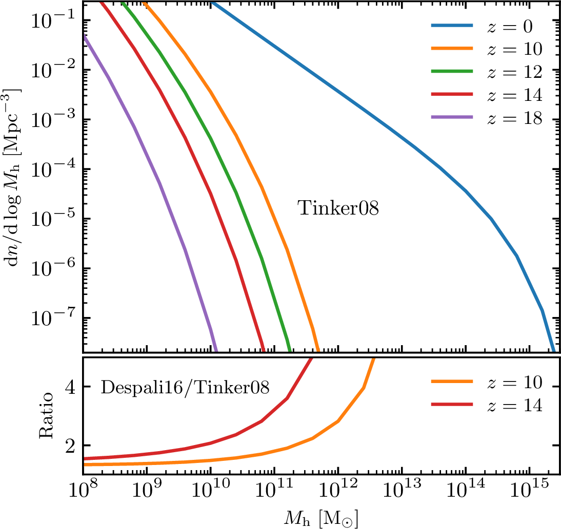
1 displays the abundance of DM halos per logarithmic mass bin per \(\, \rm Mpc^3\) at different redshifts. The plots are generated using the widely used halo mass function (HMF) outlined by [37] (hereafter Tinker08) for the \(\Lambda\)CDM cosmological model, as incorporated within the COLOSSUS cosmology Python package [38]. The curves corresponding to halos within the mass range \(M_\textrm{h}\mathrel{\rlap{\lower 4pt\hskip 0.5pt\sim} \raise 1pt>}10^{11} \, {\rm M}_\odot\) at redshifts \(z \mathrel{\rlap{\lower 4pt\hskip 0.5pt\sim} \raise 1pt>}9\) exhibit comparable abundance to large groups and clusters at \(z=0\). At the upper end of the mass range, the dependence on mass steepens significantly at such high redshifts. For instance, at \(z=9\), the abundance of halos with \(M_\textrm{h}=10^{12} \, {\rm M}_\odot\) is four orders of magnitudes lower that than halos with \(M_\textrm{h}=10^{11} \, {\rm M}_\odot\). A reasonable approximation to the HMF is given by \[\label{eq:tinker95app} \frac{{\rm d}n(z,M_\textrm{h})}{{\rm d}\log M_\textrm{h}} = \frac{10^{-5}{\, \rm Mpc}^{-3}}{\left[\left(\frac{M_\textrm{h}}{M_{-5}(z)}\right)^2+0.25 \left(\frac{M_\textrm{h}}{M_{{-5}}(z)}\right)^{0.8}(z)\right]^2}\; .\tag{3}\] The approximation is valid in the redshift range \(10<z<20\) with \(M_{-5}(z)\) is defined as, \[\log \left(M_{-5}/10^{11}\, {\rm M}_\odot\right)= 0.185(z-10)^{1.03} \; ,\] and is equal to the halo mass where \({\rm d}n/{\rm d}\log M =10^{-5}\, \rm Mpc^{-3}\). For \(M\mathrel{\rlap{\lower 4pt\hskip 0.5pt\sim} \raise 1pt>}M_{-5}(z)\), we have the steep dependence \({\rm d}n/{\rm d}\log M\sim M^{-4}\).

Various fitting formulae for the mass function are available in the literature [39]–[43]. Therefore, it is important to investigate whether discrepancies among these mass functions might be particularly notable when applied to high redshifts. The bottom panel of 1 compares the Tinker08 with another widely used HMF given in [44] (hereafter Despali16). The ratio between these HMFs increases with mass and redshift but remains within a factor of a few. Further, due to the steep dependence of the number density on halo mass, we shall see in 2 that differences in the halo mass function lead to minor changes in the estimation of halo masses by matching UV LF.

2.1 Abundance matching↩︎

[20] (hereafter H24) constrain the UV LF of high-\(z\) galaxies using 25 galaxies with spectroscopic redshifts spanning \(z\approx 8.61-13.20\). Their constraints align with various luminosity distributions derived from photometric redshifts [45]–[48]. H24 show that the observed UV LF can be effectively modeled by a double power-law function, denoted as \(\Phi_\textrm{UV}\).

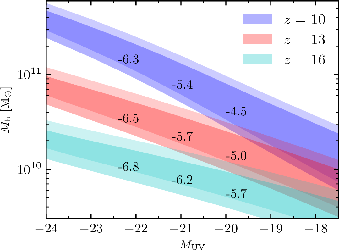
Using this double power-law fit, we conduct a straightforward abundance matching to associate galaxies with a UV magnitude, \(M_\textrm{UV}\), to halos of mass \(M_\textrm{h}\) The results of are summarized in 2 for three redshift values and for the HMFs of Tinker08 (dark shaded area) and Despali16 (light shaded). The width of each shaded area corresponds to variation in the normalization of the double power law fit, spanning a factor in between \(0.2\) and \(5\). While this should provisionally reflect the uncertainty in the measured UV LF of H24, it is important to note that the uncertainty in the observed luminosity in a single bin of one UV magnitude width could be be as large as two orders of magnitude. The results for the Tinker08 and Despali16 HMFs are remarkably consistent. This consistency is due to the steep dependence of the mass function on the mass of rare halos, approximately \(\sim M_\textrm{h}^{3.5-4}\), which implies weak sensitivity of \(M_\textrm{h}\) to the observed number of galaxies in a given UV bin.

At \(M_\textrm{UV} =-21\), the halo mass is in the range \(M_\textrm{h}=6\times 10^{10} - 1.5\times 10^{11}\, {\rm M}_\odot\) at \(z=10\), with a cumulative halo abundance (indicated by log the number density in the shaded areas) similar to massive groups and clusters at \(z=0\). Although galaxies with a fixed \(M_\textrm{UV}\) correspond to lower \(M_\textrm{h}\) as we move from low to high redshifts, the decrease in \(M_\textrm{h}\) is insufficient to maintain the same abundance. In fact, halos corresponding to a fixed \(M_\textrm{UV}\) become rarer.

At \(z\approx 10\), on average a single halo with \(M_\textrm{h}=2\times 10^{11}\, {\rm M}_\odot\) is expected in a box a \(100\, \rm Mpc\). While it is possible to employ zoom-in techniques for simulating massive halos at \(z\mathrel{\rlap{\lower 4pt\hskip 0.5pt\sim} \raise 1pt>}10\), this necessitates significant computational resources. Instead, we adopt a computationally friendlier approach, utilizing constrained random realizations to generate initial conditions that are guaranteed to contain a massive halo when evolved forward to a specified redshift, \(z\).

3 Simulations↩︎

In 3.1, we outline the method for generating constrained initial conditions. Using these initial conditions, simulations of DM particles were conducted in periodic boxes using the SWIFT cosmological code [49]. All simulations started at redshift \(z_{i}=80\) and concluded at \(z=9\). As we shall see below, the linear density contrast corresponding to the constraint is \(\delta_c=1.68\) at \(z=9\), and hence the corresponding density at the initial redshift \(z_i\) is \(0.02\), well within the linear regime. Furthermore, to capture any mild deviations from linear evolution at \(z_i\), the initial conditions are generated using the Zel’dovich approximation, rather than linear theory.

We performed nine simulations constrained to have halo masses of approximately \(M_\textrm{h}\approx 10^{11}\, {\rm M}_\odot\) in boxes of \(L=17.1 \, \rm Mpc\), along with one unconstrained simulation in a box of the same size. Additionally, two simulations were conducted with initial conditions constrained to include a halo mass of \(M_\textrm{h}\approx 10^{12}\, {\rm M}_\odot\) at \(z=9\), positioned at the center of cubic boxes of \(L=36.9 \, \rm Mpc\).

Each simulation consisted of \(512^3\) equal-mass particles, resulting in particle masses of \(10^7\, {\rm M}_\odot\) and \(10^6 \, {\rm M}_\odot\) in the large and small boxes, respectively. The maximum physical softening used in the simulations was \(100\ {\rm pc}\). Throughout each simulation run, the output of positions and velocities of all particles was retained at 18 different redshifts spanning from \(z=20\) to \(z=9\). Halos were identified from the simulation outputs utilizing the VELOCIraptorhalo finder [50]. This halo finder provides halo masses according to several definitions. Here we use VELOCIraptormasses that match the definition in 1 .

3.1 Constrained Initial Conditions↩︎

We formulate the condition (constraint) for the presence of a halo of a given mass as follows. Let \(\delta(\mathbf{x},z)\) be the linearly evolved density at redshift \(z\) and \(\delta_R(\mathbf{x},z)\) be its convolution with a top-hat window of comoving radius \(R\). We associate a halo of mass \(M_\textrm{h}\) with a comoving Lagrangian radius \(R_L=(3M_\textrm{h}/4\pi\rho_\textrm{m})^{1/3}\), where \(\rho_\textrm{m}\) is the background density in comoving coordinates.

The formation of a halo of mass \(M_\textrm{h}\) at redshift \(z\), located at position \(\mathbf{x}_0\) is determined by the condition \(\delta_{R=R_L}(\mathbf{x}_0,z)=\delta_c\simeq 1.68\) [51], [52]. Here, \(\delta_c\) is the critical threshold indicative of the virialization of DM halos. At \(z=10\), halos with masses \(M_\textrm{h}=10^{11}\, {\rm M}_\odot\)and \(M_\textrm{h}=10^{12}\, {\rm M}_\odot\)correspond to Lagrangian comoving radii of \(R_L=0.84 \, \textrm{Mpc}\) and \(1.82 \, \textrm{Mpc}\), respectively. In terms of the ratio \(\delta_c/\sigma_{R_L}\), these are equal to \(4.8\) and \(6.5\), providing a measure of halo formation likelihood under the specified conditions. This formulation is only approximate as the superposition of generic fluctuations on all scales and non-linear evolution will lead to deviations from the desired halo mass and position. Nonetheless, the prescription is reasonable for massive (rare) halos [53], [54], as is the case in the current study.

We adopt the methodology of [33] to generate gaussian random fields that satisfy the aforementioned condition. This method expresses the constrained random field, denoted by \(\delta_1\), in terms of an unconstrained random gaussian field, \(\delta^\textrm{unc}\), as follows \[\label{eq:hr1} \delta_1(\mathbf{x},z) = \delta^\textrm{unc}(\mathbf{x},z)-\langle \delta(\mathbf{x},z)|{\delta_{R_L}^\textrm{unc}}\rangle+\langle\delta(\mathbf{x},z)|{\delta_c}\rangle\;\tag{4}\] where \({\delta_{R_L}^\textrm{unc}}\) is the value of the filtered unconstrained field at \(\mathbf{x}_0\). The ensemble average of all \(\delta\) fields satisfying the constraint \(\delta_{R_{L}}(\mathbf{x}_0,z)=C\) is given by \[\label{eq:HR} \langle \delta(\mathbf{x})|C \rangle = \zeta(|\mathbf{x} - \mathbf{x}_0|) \frac{C}{\sigma_{R_L}^2}\; ,\tag{5}\] where \(\sigma^2_{R_L}\) is the variance of the smoothed density, \(\delta_{R_L}\).

3.2 Results↩︎

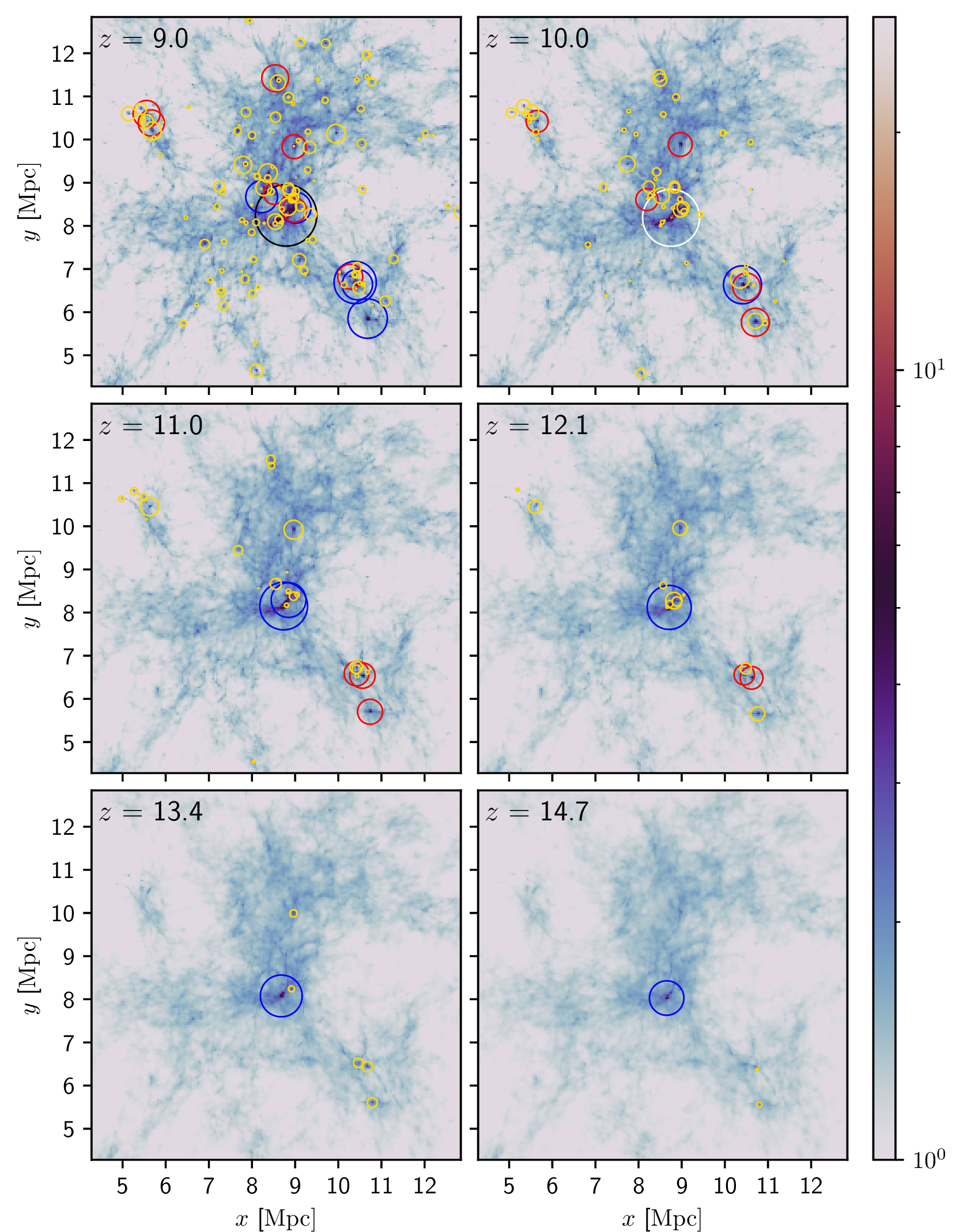
3 illustrates the projected (2D) density (in units of the mean 2D density value) for one of the \(M_\textrm{h}=10^{11}\, {\rm M}_\odot\)constrained simulations. The overlaid circles represent identified halos in different mass ranges, as described in the figure caption. Only halos above \(10^9\, {\rm M}_\odot\) are marked.

The displayed region of the box is focused around the center. As expected, the most massive halo (MMH) forms near the center. Additional massive halos are associated with the growth of the MMH, however, their masses are significantly lower than the MMH. Halos in the mass range \(5\times 10^9<M_\textrm{h}/\, {\rm M}_\odot<10^{10}\) (red circles) are present at \(z\simeq 12\). These halos are not considered rare, as their expected abundance is \(10^{-2}-10^{-3} \textrm{dex}^{-1} \, \rm Mpc^{-3}\) (see 1). Therefore, we expect to identify a few such halos even in our simulation box of \(L=17.1 \, \rm Mpc\).

Inspection of the panels at \(z=11\) and \(z=10\) reveals a major merger event with the two halos marked by two blue circles (\(10^{10}<M_\textrm{h}/\, {\rm M}_\odot<5\times 10^{10}\)) at \(z=11\) merging to form the larger halo indicated by the white circle (\(5\times 10^{10}<M_\textrm{h}/\, {\rm M}_\odot<10^{11}\)) at \(z=10\). There is a clear tendency of increasing halo mass as we move nearer to the MMH, particularly at the lowest redshifts.

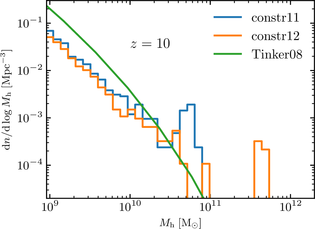
4 shows the abundance of halos from the simulations as a function of \(M_\textrm{h}\). At the high mass end, the simulated abundance significantly exceeds the predictions from the Tinker08 fitting formula (green curve). In both \(M_\textrm{h}=10^{11}\, {\rm M}_\odot\)and \(M_\textrm{h}=10^{12}\, {\rm M}_\odot\)constrained simulations, the MMH is accompanied by other relatively rare massive halos with abundance well above the green curve. The initial condition constraint ensures a massive halo in a small region, making the simulation box atypical for its volume. Consequently, the number density of massive halos in the simulation significantly exceeds the expected mean, explaining the enhanced abundance of high \(M_\textrm{h}\) halos compared to Tinker08. One pathway for the formation of these massive halos is through the accretion of smaller halos, leading to a modest depletion in the low \(M_\textrm{h}\) range. This explains why the simulated halo abundance at low \(M_\textrm{h}\) falls slightly below the green curve, typically by a factor of \(3-4\).

3.2.1 Halo Accretion History↩︎

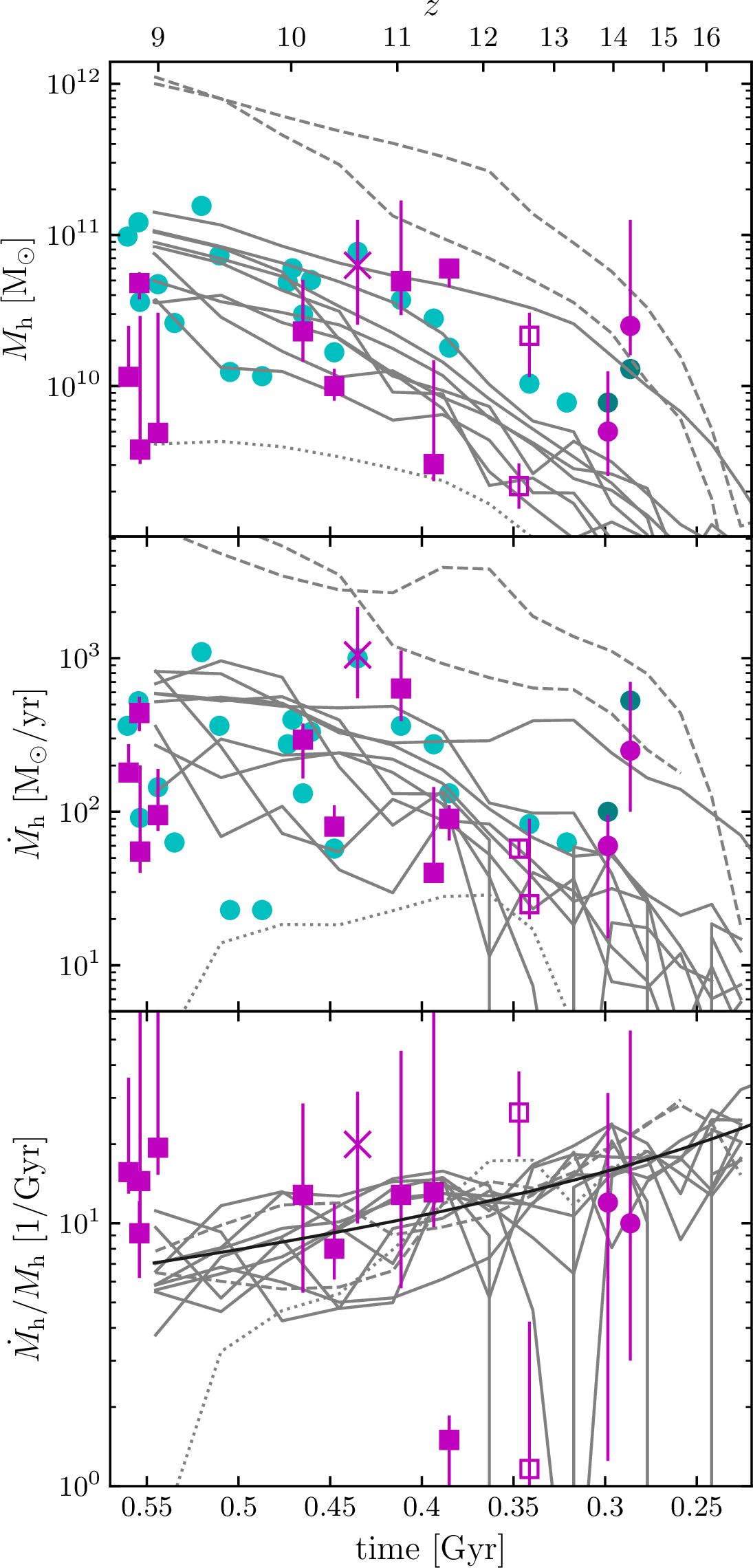
5 displays the evolution of MMH properties in simulations (continuous curves) and compares them with observational data (individual symbols). The figure is divided into three panels, each focusing on a different aspect of halo growth. The data symbols are as follows.

• Magenta symbols with error bars are based on stellar masses and SFRs inferred via SED fitting. The filled squares are taken from table 3 in H24. The open squares refer to the galaxy GS-z12 for which different values of redshift, SFR and \(M_\ast\) are reported in [55] and H24. Both sets of data are shown, with [55] being the point with the lower redshift (\(z=12.43\)). The cross is the galaxy GN-z11 [56]. The two highest redshift points represented by filled circles correspond to the two galaxies reported in [57].

  The observed stellar mass, \(M_*\), and SFRs, \({\dot{M}}_*\), are used to estimate halo masses and mass accretion rates assuming assuming \[\label{eq:mst95to95mh} M_\textrm{h}=f_\textrm{b}^{-1} f_\textrm{SF}^{-1} M_\ast= 50\left(\frac{0.13}{f_\textrm{SF}} \right) M_*\; ,\tag{6}\] and similarly for the relation between \({\dot{M}}_\textrm{h}\) and \({\dot{M}}_*\). As before, \(f_b\) is the global barynonic mass fraction, and the star formation efficient \(f_\textrm{SF}\) is a constant assigned a default value \(f_\textrm{SF}=0.13\), implying \(M_\textrm{h}=50 M_*\)

• Cyan circles are based solely on the observed \(M_\textrm{UV}\) provided in table 1 of H24. The dark cyan circles correspond to the two highest redshift galaxies, with \(M_\textrm{UV}\) taken from [57]. For these points, halo masses are inferred from \(M_\textrm{UV}\) via abundance matching from the observed UV magnitudes. From 2, the relative uncertainty in these points is a factor of \(\approx 2-3\), but we do not attach the corresponding error bars for the sake of clarity. The SFRs are deduced directly using \({\dot{M}}_\ast(\textrm{M}_\odot \, \textrm{yr}^{-1})= 1.15 \times 10^{-28} L_{UV}(\mathrm{erg\, s^{-1} \,Hz^{-1}}\) assuming a Salpeter IMF. The halo accretion rate is them estimated from 6 .

Top panel: halo mass vs. time. The grey curves correspond to \(M_\textrm{h}(t)\) of the simulated MMHs. The curves reveal that half of the simulated MMHs, including the unconstrained halo (dotted), have acquired 80% of their final masses in the last \(150 \, {\rm Myr}\). Only the dashed curves, corresponding to constrained simulations with \(M_\textrm{h}\approx 10^{12}\, {\rm M}_\odot\) and one of the nine solid curves, have acquired a mass \(\gtrsim 10^{10} \, {\rm M}_\odot\) by \(z=15\).

The Cyan circles fall within the range of solid curves corresponding to simulations constrained to contain a \(M_\textrm{h}\approx 10^{11}\) halo. The result is not entirely trivial since \(M_\textrm{h}\) of the MMHs been tuned to match the abundance at redshifts \(z\approx 9\) and not at higher redshifts. Indeed, at higher redshifts, the spread in halo masses between different simulations is becomes large, ranging from \(M_\textrm{h}\approx 10^{10}\, {\rm M}_\odot\) to \(10^{11}\, {\rm M}_\odot\) even at at \(z=10\), as indicated by the solid curves. This mass range is associated with more than a two-order-of-magnitude difference in the abundance of halos, as shown in 1.

The highest redshift data point represented by a magenta circle is well above all solid curves except one (yellow curve). Nonetheless, since we have only nine curves corresponding to the \(M_\textrm{h}=10^{11}\, {\rm M}_\odot\)simulations, we conclude that this data point is consistent with simulated accretion history.

At \(z\mathrel{\rlap{\lower 4pt\hskip 0.5pt\sim} \raise 1pt>}10\), the estimates from 6 (magenta) agree with both the \(M_\textrm{h}=10^{11}\, {\rm M}_\odot\)simulations and abundance matching results (cyan circles). However, at \(z\simeq 9\), these estimates fall below both simulations and abundance matching. This is in agreement with various models in the literature [18], [20], [58], [59] predicting an LF consistent with the observations at \(z~\rlap{<}{\lower 1.0ex\sim}9\), but underestimating the observed abundances at \(z\mathrel{\rlap{\lower 4pt\hskip 0.5pt\sim} \raise 1pt>}11\).

Middle panel: mass accretion rate. As in the previous panel, the curves correspond to the simulations. The \({\dot{M}}_\textrm{h}\) curves reveal significant variations between individual halos. Some halos exhibit highly fluctuating \(M_\textrm{h}\), while others (e.g., those represented by dashed and a few solid curves) show smoother evolution. However, even these smoother curves display fluctuations on timescales \(~\rlap{<}{\lower 1.0ex\sim}100\, {\rm Myr}\).

The magenta and cyan points agree with each other, but are not identical, as the SED fitting involves more detailed SFR modeling than UV magnitudes alone. Accretion rate curves from the \(M_\textrm{h}=10^{11}\, {\rm M}_\odot\)simulations are consistent with observations via \(M_\textrm{UV}\) (cyan) and SED-SFRs (magenta).

We emphasize that while both cyan and magenta points in top and middle panels rely on \(M_\textrm{UV}\), their methodologies differ: abundance matching for the top panel versus an empirical SFR-\(M_\textrm{UV}\) relationship for the middle panel.

Bottom panel: specific accretion rate. The specific halo accretion rates, \({\dot{M}}_\textrm{h}/M_\textrm{h}\), from simulations cluster around a simple fit denoted by a black line, represented by the equation \({{\rm d}{\rm ln}M_\textrm{h}}/{{\rm d}t} = 3.15 t_{\textrm{Gyr}}^{-4/3} \, {\rm Gyr}^{-1}\). This fit approximates the mean accretion rate for halos of mass \(M_\textrm{h}=10^{11}\, {\rm M}_\odot\) as proposed by [60].

The magenta points represent the sSFR, \({\dot{M}}_*/M_*\), from observations. Cyan circles are absent from this panel since only \({\dot{M}}_*\) can be directly derived from \(M_\textrm{UV}\).

At \(z>10\), there is a reasonable agreement between the observed sSFRs and the halo accretion rates from the simulations. This consistency corroborates the findings of [48], who noted that the sSFRs tend to follow the scaling \((1+z)^{2.5}\) proposed by [60] for the specific halo accretion rate at high redshift. However, the normalization of the specific halo accretion rate in [48] is higher by a factor of a few compared to the fit by [60].

At \(z<9\), the discrepancy between data and observations seen on the top panel is also evident here. While reducing \(f_\textrm{SF}\) by a factor of \(\approx 5-10\) (from \(f_\textrm{SF}=0.13\) to \(0.01-0.025\)) would reconcile the \(z\simeq 9\) with the \(M_\textrm{h}\) results in the top panel, it would not effect the halo specific accretion rate (assuming a constant \(f_\textrm{SF}\)). The is because, according to 6 , the specific accretion rate is equal to the sSFR, i.e. \({\dot{M}}_\textrm{h}/M_\textrm{h}=\dot{M}_\ast/M_\ast\), independently of \(f_\textrm{SF}\).

Note that \(M_\ast\propto M_\textrm{h}^\alpha\) (\(\alpha=const\)), then \({\dot{M}}_\textrm{h}/M_\textrm{h}=\alpha^{-1} \dot{M}_\ast/M_\ast\) [58]. Therefore, also for \(\alpha\ne 1\) curves of the sSFR and the specific halo accretion rate should trace each other, with a constant ratio between them. Thus, a mass-dependent \(f_\textrm{SF}\) would not resolve the discrepancy.

4 Boosting the star formation efficiency at high-\(z\)↩︎

A boost in \(f_\textrm{SF}\) to \(\approx 0.13\) at high-\(z\) yields reasonable agreement between simulated halos and observations, representing a mild increase relative to low-\(z\). We present a simple recipe explaining this enhancement, suggesting that star formation processes may not significantly differ across redshifts. We present a model explaining this enhancement, arguing that star formation processes may not significantly differ across redshifts. For a halo of mass \(M_\textrm{h}(t_z)\) at redshift \(z\), we model \(M_\ast\) and \(\dot{M}_\ast\) assuming star formation occurs in a rotationally supported disk governed by the Schmidt-Kennicutt (SK) law [61], [62]: \[\label{eq:SK} {\dot{\Sigma}}_\ast =A \Sigma_{g}^n ; ,\tag{7}\] where \({\dot{\Sigma}}_\ast\) is the SFR per unit disk area, \(n=1.54\), and \(A=10^{-3.95}\) [63]. \(\Sigma_\ast\) and \(\Sigma_{g}\) are in \(\textrm{M}_\odot ,\textrm{pc}^{-2}\). Disk gas partially converts to stars following the SK law, with stellar feedback expelling a fraction. The disk gas reservoir is simultaneously replenished and expanded through halo accretion.

The gas surface density evolution is described by, \[\label{eq:mass95balance} {\dot{\Sigma}}_g = {\dot{\Sigma}}_\textrm{acc}- {\dot{\Sigma}}_\ast -{\dot{\Sigma}}_\textrm{ej} \; ,\tag{8}\] where \({\dot{\Sigma}}_\textrm{acc}\) is accretion, \({\dot{\Sigma}}_\ast\) is star formation, and \({\dot{\Sigma}}_\textrm{ej}\) is feedback-driven ejection. For halos with \(M_\textrm{h}~\rlap{<}{\lower 1.0ex\sim}10^{12}M_\odot\), AGN feedback is subdominant [64]–[66].

Gas ejection is modeled via [11], [67]–[69], \[\label{eq:eject} {\dot{\Sigma}}_\textrm{ej}= \left(\frac{V_c}{V_{SN}}\right)^{-\gamma}{\dot{\Sigma}}_\ast \; ,\tag{9}\] with \(V_{SN}=240\, {\rm km }\, {\rm s}^{-1}\) and \(\gamma = 2.8\) [69]. This implies more effective stellar feedback in halos with shallow gravitational potential [9], [10].

The accreted gas mass in time \(\delta t\) is, \[\label{eq:dmacr} \delta M_\textrm{acc}=f_\textrm{b}{\dot{M}}_\textrm{h}\delta t\; .\tag{10}\]

Due to short crossing times and efficient cooling [18], [70], we assume rapid settling into an exponential disk: \[\label{eq:dsacr} \delta \Sigma_\textrm{acc}(t,R) = \delta \Sigma_0 e^{-R/R_d(t)}\; ,\tag{11}\] where \(R_\textrm{d}= 0.7 \lambda_\textrm{B}r_\textrm{h}\) [71], [72], and \(\lambda_\textrm{B}\) is the halo spin parameter [73]. Therefore, \[\label{eq:dSacr} {\dot{\Sigma}}_\textrm{acc}(t,R) = \frac{f_\textrm{b}\dot{M}_\textrm{h}}{2\pi R_\textrm{d}^2(t)} e^{-R/R_\textrm{d}(t)}\; .\tag{12}\]

Motivated by our simulations, we assume \({\dot{M}}_\textrm{h}/M_\textrm{h}\propto t^{-4/3}\), yielding: \[\label{eq:mh95fit} M_\textrm{h}(t)=M_\textrm{h}(t_z) \mathrm{e}^{A(t_z^{-\beta}-t^{-\beta})}; ,\tag{13}\] where \(A=-8.1\), \(\beta= 1/3\), and \(t\) is in Gyr.

We numerically integrate 7 12 from \(t=t_i\ll t_z\) to \(t=t_z\). Initial conditions are set as \(\Sigma_{\ast}(t_i,R)=10^{-3}\Sigma_{g}(t_i,R)\), with \(\Sigma_{g}(t_i,R)\) following an exponential profile. \(R_\textrm{d}(t_i)\) is determined by \(R_\textrm{d}= 0.7 \lambda_\textrm{B}r_\textrm{h}\) with \(r_\textrm{h}=r_\textrm{h}(t_i)\). The initial disk gas mass equals \(f_\textrm{b}M_\textrm{h}(t_i)\) minus the initial stellar mass. We use \(\lambda_\textrm{B}=0.035\) in all calculations.

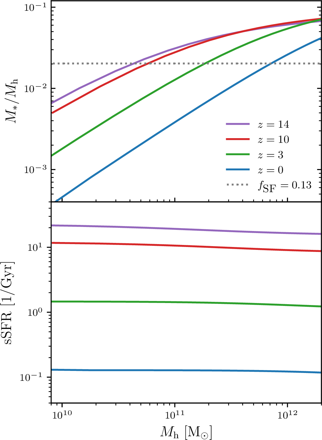
In the top panel of 6, the SHMR is plotted against halo mass for four redshift values, \(z\). The model agrees reasonably well with the observed local SHMR as estimated through abundance matching techniques [24]–[26], [74], [75].

The model SHMR acquires larger values at higher redshifts for a given mass. This is due to the relation \(V_c \sim M_\textrm{h}/t\), indicating that a higher circular velocity \(V_c\) occurs at earlier times for a fixed \(M_\textrm{h}\), leading to less efficient SN feedback and, consequently, a larger gas reservoir for star formation. The SHMR for \(M_\textrm{h}\approx 10^{11} \, {\rm M}_\odot\) increases by approximately a factor of five at high-\(z\) compared to \(z=0\), while for \(10^{10} \, {\rm M}_\odot\), the increase is about a factor of 25. In contrast, predictions from the UniverseMachine [76] suggest that the SHMR increases by about a factor of 10 from \(z=0\) to \(z=12\) for halos with \(10^{10} \, {\rm M}_\odot\) (their figure 12).

The SHMRs change very little between \(z=10\) and \(14\) with a weak dependence on \(M_\textrm{h}\). For the relevant mass range \(M_\textrm{h}\approx 5 \times 10^{10}- 10^{11}\, {\rm M}_\odot\) the SHMR is \(\approx 2\%\) corresponding to \(f_\textrm{SF}\approx 0.13\), the value used in figure 5.

For \(M_\textrm{h}\approx 10^{11}\, {\rm M}_\odot\), at \(z=3\), the SHMR changes by a factor of \(\approx 4-5\) compared to \(z=0\). This may seem at odds with observational analyses in the literature, which generally suggest a constant SHMR over this redshift range. We defer a detailed discussion of this issue to §5.

The sSFRs plotted in the bottom panel are close to the observed values at the corresponding redshifts [48] and depends weakly on \(M_\textrm{h}\).

These results suggest that the enhanced star formation efficiency in high-\(z\) galaxies can be explained by the fundamental physics of structure formation and feedback processes, without invoking drastically different star formation mechanisms compared to the local universe.

5 summary and discussion↩︎

We have presented a study of the accretion history of massive halos at redshifts \(z\gtrsim\), relevant to luminous galaxies observed at such high redshifts. Our approach is based on constrained simulations, which is highly beneficial for studying rare cosmological structures. Here we have only conducted simulations with constant resolution across the entire simulation box. However, a combination of zoom-in techniques and constrained initial conditions is most appropriate for resolving rare structures as well as capturing the gravitational influence of the large scale environment.

Growing evidence suggests highly variable star formation history at high redshifts [77], [78], potentially due to mergers, interactions, and environmental conditions. This variability could bias inferred UV luminosity distributions [21], [30], [79]–[81], as galaxies in low-mass halos may be preferentially detected during increased star formation phases. In the simulations, individual halo accretion curves exhibit both long-term fluctuations (\(\mathrel{\rlap{\lower 4pt\hskip 0.5pt\sim} \raise 1pt>}100 \, {\rm Myr}\)) and short-term variations. Examining 5 (middle panel) reveals a tendency for greater variability in lower mass halos at \(z=9\) compared to more massive ones, potentially leading to enhanced stochasticity in associated star formation rates. However, our output times do not capture variability at \(~\rlap{<}{\lower 1.0ex\sim}10 \, {\rm Myr}\) scales.

High-resolution simulations yield mixed results: SERRA simulations do not produce sufficient star formation rate variability [31], while FIRE-2 simulations show bursty star formation that explains the observed UV luminosity function (LF) [30]. However, stellar masses at \(z\mathrel{\rlap{\lower 4pt\hskip 0.5pt\sim} \raise 1pt>}10\) in these simulations [82] are lower than observed estimates from spectroscopically confirmed galaxies [20]. Nonetheless, stochasticity is clearly an important effect that should be considered.

In 5 we have seen that dividing the observed SFRs by a factor \(f_b f_\textrm{SF}=2\%\) (i.e. \(f_\textrm{SF}=0.13\)), leads to \({\dot{M}}_\textrm{h}\) that are consistent with the simulations constrained to include a halo of mass \(M_\textrm{h}\approx 10^{11} \, {\rm M}_\odot\). The agreement spans the entire considered redshift range, \(z>9\). Interestingly, dividing the observed stellar masses by the same factor yields a good match with the halo masses in the simulations, but this is only true for \(z\gtrsim 10\). For galaxies at \(z\simeq 9\), the factor required is smaller by a factor of \(\approx 5-10\) (\(f_\textrm{SF}\approx 0.025-0.01\)), closer to what is seen in low redshift galaxies.

This peculiar behaviour of the inferred \(M_\textrm{h}\) between \(z\approx 9\) and \(z\approx 10\) may stem from challenges in accurately estimating the stellar masses. Indeed, SFRs estimated from UV magnitudes are generally more reliable than stellar mass estimates, which require assumptions about the entire star formation history [83] SED fitting [31], [83]–[86]. A striking example is the galaxy GS-z12 (\(z=12.48\)). Its estimated mass varies by an order of magnitude depending on the method used: \(M_\ast = 4.3^{+1.8}_{-2} \times 10^8 \, {\rm M}_\odot\) using PROSPECTOR [20], [87] and \(M\ast = 4.36^{+1.8}_{-1.27}\times 10^7 \, {\rm M}_\odot\) using BEAGLE [55], [88]. Nonetheless, in the estimating the SFRs, the impact of potential uncertainties due to potential dust attenuation needs to be assessed [89]. However, dust attenuation is expected to be small in these high redshift galaxies [48], suggesting that the observed discrepancies could primarily be due to the complexities of stellar mass estimation.

Another possibility for this behaviour is an abrupt change in the conditions for star formation at \(z\approx 9-10\), similar to the suggestion of [90] although their model refers to transition at \(z\approx 6\).

Numerical simulations are computationally intensive for tracing the accretion history of a large ensemble of halos. Semi-analytic methods for generating constrained merger histories [91] offer a CPU-efficient alternative. These could be valuable for exploring variations in past accretion rates of rare halos at high redshifts. Currently, these methods have been applied to trace the growth of rare halos from \(z\approx 12\) to \(z=0\), rather than tracing rare halos at \(z\approx 10\) backward in time.

Numerous models aim to understand the formation of luminous high-\(z\) galaxies. [47] suggested that UV-inferred SFRs might be overestimated due to a top-heavy IMF at high redshift, which could arise naturally in low-metallicity environments. [18] noted this could account for a factor of 4 boost in UV luminosities, aligning their semi-analytic models with observations. [70] propose conditions for feedback-free star formation in \(\approx 10^7\, {\rm M}_\odot\) gas clouds at high redshifts, satisfied in \(10^{11}\, {\rm M}_\odot\) halos at \(z\approx 10\). Conversely, [90] invoke AGN positive feedback, suggesting short-lived AGN activity triggers vigorous star formation via momentum-conserving outflows. They predict a transition to energy-conserving flows at \(z\approx 6\), leading to gas depletion and quenched star formation at lower redshifts. [92] propose that decreased dust attenuation at high redshifts could explain the abundance of \(z\gtrsim 10\) galaxies, compensating for reduced host halo abundance. Modifications to the primordial mass power spectrum have also been explored [93]–[96].

In the approximate star formation recipe outlined in §4, we used the halo’s circular velocity, \(V_c\), as the parameter governing SN feedback. Combined with the local KS law, the recipe aims to demonstrate that negative feedback at high-\(z\) is naturally expected to be less efficient than at lower \(z\).

According 6 the recipe implies an evolving SHMR at moderate redshifts and a non-evolving one at \(z\gtrsim 10\). Observationally, within the uncertainties, a non-evolving SHMR is generally consistent with galaxy luminosity distributions up to \(z ~\rlap{<}{\lower 1.0ex\sim}5\). However, for the redshift range \(z \approx 0 - 10\), studies in the literature show divergent results. Some find weak to moderate redshift dependence [24], [25], [74], [97], [98], while others report significant evolution [99]–[101]. Notably, substantial differences exist between various SHMR estimates at similar redshifts and halo masses.

The evolution of the SHMR, inferred through abundance matching techniques, is sensitive to various factors, including the shape of the galaxy stellar mass function [102]. As highlighted by [27], uncertainties in observed stellar mass functions at redshifts \(z\lesssim 4\) can lead to differing interpretations regarding the evolution of the SHMR from \(z=0\) to \(z=4\). Depending on specific assumptions about the stellar mass function, the SHMR could exhibit either a decrease or an increase over this redshift range. Depending on the assumptions, the SHMR for a halo with \(M_\textrm{h}\approx 10^{11} \, {\rm M}_\odot\) could vary by two orders of magnitude due to different assumptions.

The recipe in §4 can be adapted to yield a nearly non-varying SHMR at \(z\lesssim 5\) through several modifications. For example, the adopted expression for \(M_\textrm{h}(t)\) is approximate and neglects variations between halos, which can be significant according to 5. The expression motivated by our high-\(z\) simulation results. A recipe with slower accretion at moderate redshifts would yield a less varying SHMR at \(z\lesssim 5\).

Furthermore, following [69], we have adopted a gas ejection expression determined by \(V_c\). However, the maximum circular velocity (the peak of the rotation curve), \(V_{\textrm{max}}\), is likely more relevant since it better reflects the depth of the gravitational potential of the halo.

In the regime of stable clustering, \(V_{\textrm{max}}\) is expected to remain constant over long cosmic epochs. Thus, employing \(V_{\textrm{max}}\) instead of \(V_c\) in the model should result in a more constant SHMR over extended periods. We have run the recipe with \(V_\textrm{max}\) instead of \(V_c\) in 9 , where the dependence on \(M_\textrm{h}\) and \(z\) follows the formula obtained by [103] by fitting the median growth of halos in MultiDark N-body simulations. This has yielded closer curves for the SHMR at \(z=0\) and \(z=3\), while leaving the curves at \(z=10\) and \(14\) virtually unchanged.

6 Data availability↩︎

New numerical simulation data have been generated and analyzed.

7 acknowledgements↩︎

The author has benefited from fruitful conversations with Andrew Benson, Enzo Branchini, Stephane Charlot, Avishai Dekel and Joe Silk. This research is supported by a grant from the Israeli Science Foundation and a grant from the Asher Space Research Institute. The research in this paper made use of the SWIFT open-source simulation code (http://www.swiftsim.com, [104]) version 1.0.0.

References↩︎