Bounded-Confidence Models of Opinion Dynamics with Neighborhood Effects
February 08, 2024
Abstract
People are influenced by the people with whom they interact. As their opinions change, their social networks typically coevolve with them. People are often more susceptible to influence by people with similar opinions than by people with dissimilar opinions. In a bounded-confidence model (BCM) of opinion dynamics, interacting individuals influence each other through dyadic influence if and only if their opinions are sufficiently similar to each other. In the present paper, we introduce “neighborhood BCMs” (NBCMs) that include both the usual dyadic influence and a transitive influence, which models the effect of friends of a friend when determining whether or not an interaction with a friend influences an individual. In this transitive influence, an individual’s opinion is influenced by a neighbor when, on average, the opinions of the neighbor’s neighbors are sufficiently similar to their own opinion. We formulate both neighborhood Deffuant–Weisbuch (NDW) and neighborhood Hegselmann–Krause (NHK) BCMs. We simulate our NDW model on time-independent networks and find that it can yield interesting opinion states, such as opinion jumping and pseudo-consensus, that cannot occur in an associated baseline DW model. We also simulate our NDW model on adaptive networks that coevolve with opinions by changing its structure through “transitive homophily". In this network evolution, an individual that breaks a tie to one of its neighbors and then rewires that tie to a new individual, with a preference for individuals with a mean neighbor opinion that is closer to that individual’s opinion. We explore how the qualitative opinion dynamics and network properties of our time-independent and adaptive NDWM models change as we adjust the relative proportions of dyadic and transitive influence. Finally, we study a two-layer opinion–disease model in which we couple our NDW model with disease spread through a shared adaptive network that can change both on the opinion layer (e.g., by breaking ties through disagreement) and on the disease layer (e.g., through quarantining), and we examine how the opinion dynamics affect disease spread.
1 Introduction↩︎
Social interactions, human opinions, and human behavior influence each other in inextricable ways. Moreover, social interactions typically follow the principle of homophily, as individuals tend to interact more with individuals who are similar to themselves than with those who differ from them [1]. Human opinions, and the manner and time scales over which they evolve, play an important role in many real-world settings, such as decision-making[2], misinformation and disinformation campaigns [3], referendums [4], and political polarization [5].
There are myriad models of opinion dynamics [6], [7], which encode opinions and how they evolve in a variety of ways. Some opinion models (e.g., voter models [8]) have discrete-valued opinions and other opinion models have continuous-valued opinions. Models with continuous-valued opinions include the DeGroot consensus model [9], [10], the Friedkin–Johnson model [11], bounded-confidence models (BCMs) [12], [13], and models with explicit radicalization dynamics [14]. Much of the literature on opinion dynamics has focused on conditions for consensus, in which opinions converge to a single value, but it is also important to study phenomena such as polarization (in which there are two major opinion clusters), fragmentation (in which there are three or more major opinion clusters), and others.
In a traditional BCM, interacting agents interact and change their opinions if and only if their current opinions are sufficiently similar. Two agents influence each other if the difference between their opinions lies within a confidence bound. The two foundational BCMs are the Hegselmann–Krause (HK) model (which uses synchronous updates of agent opinions) [15] and the Deffuant–Weisbuch (DW) model (which uses asynchronous opinion updates) [16]. In the HK model, interactions take place in groups, with each agent changing their opinion to the mean of the opinions of their neighboring agents whose opinions are within the confidence bound. By contrast, in the DW model, interactions are pairwise (i.e., dyadic), with a single pair of agents interacting at each discrete time. If the difference between their opinions lies within the confidence bound, they compromise their opinion by some amount when they interact. Extensions of BCMs include models that incorporate leaders [17], stubborn agents [18], heterogeneous confidence bounds [19], smooth interactions (e.g., through sigmoidal functions) [14], [20], BCMs with coevolving opinions and networks [21], [22], and polyadic agent interactions (i.e., with three or more agents interacting simultaneously) instead of only dyadic ones [23], [24].
By studying BCMs on networks, researchers examine how network structure influences opinion dynamics [25]. Most BCMs consider only direct influence, in the sense that interact agents only consider each other’s opinion when determining whether or not to update their opinion. However, humans are influenced not only directly but also through transitive influence (e.g., through friends of friends) [26]. They are thus influenced by neighbors of adjacent agents. Such transitive influence is notably prevalent in interactions on social media [27], which has low barriers to interacting with friends of friends. Moreover, individuals can be influenced not only by the friends of their friends (i.e., individuals who are two steps away), but also by individuals who are even farther away in a network. In their studies of influence on social networks, Nicholas Christakis and James Fowler [28] have posited the idea of “three degrees of influence" to illustrate how many steps away from an agent in a network yield robust influence on their behavior and opinions. Researchers have also noted the importance of extended neighborhoods in empirical network data (e.g., in Facebook [29]) and in the design of algorithms (e.g., for local community detection [30]).
In the present paper, we study opinion models that capture transitive influence from friends of friends. We formulate neighborhood BCMs (NBCMs), in which an agent can change its opinion based both on dyadic interactions with adjacent nodes and on the mean opinion of the neighbors of those adjacent nodes. We refer to this mean opinion as the “mean neighbor opinion". For the dyadic influence, we employ the usual confidence bound of BCMs, so two interacting agents compromise their opinions by some amount if they are sufficiently similar to each other (i.e., if their opinions differ by less than a confidence bound). The two agents also experience transitive influence, in which an agent is influenced by an agent with whom it interacts if that agent’s mean neighbor opinion is within the confidence bound (i.e., if the mean opinion of its neighboring nodes is sufficiently similar). Although the mean neighbor opinion influences whether or not an agent updates its opinion, the magnitude of opinion changes are affected only by the opinion of the interacting agents themselves. We explore the qualitative behavior of our NBCMs for different relative proportions of direct influence (i.e., through dyadic interactions) and transitive influence (i.e., through neighborhood effects). Because of the transitive influence (and unlike in conventional BCMs), a node in our NBCMs can update its opinion due to an interaction with an adjacent node without requiring that the adjacent node also update its opinion, even when both nodes have the same confidence bound. In particular, this asymmetry can arise when all nodes have the same constant confidence bound. Additionally, because of transitive influence, two interacting nodes can influence each other even when their opinions differ by more than the confidence bound.
We are not aware of any existing BCMs that consider such neighborhood effects. However, there does exist a DeGroot model [31] in which agents update their opinions so that they are closer to the opinions of agents that are neighbors of neighbors. The neighborhood effects in our NBCMs model transitive homophily (i.e., neighborhood-based homophily) and differ in a key way from the neighborhood effects in [31]. In our model, changes in opinions are based only on the opinions of their neighbors (i.e., by agents that are one step away in a network and hence are adjacent to them). However, neighbors of neighbors (i.e., agents that are two steps away) influence whether or not an agent changes its opinion in the first place. Our NBCMs also inherit the desirable property that individuals have heterogeneous tolerances towards others’ opinions. Notably, this heterogeneity arises even when for a constant, homogeneous confidence bound.
Changes in opinions can lead to changes in relationships between agents, which in turn can lead to changes in the structure of a network. See [32] for a review of coevolving (i.e., adaptive) network models. A variety of adaptive-network models have been developed to study the coevolution of opinions and network structure. Examples include adaptive voter models [33], [34], adaptive BCMs and related opinion models [21], [22], [35]–[37], and others. In an adaptive opinion model, there is typically a mechanism for agents to remove ties to agents with whom they disagree (or with whom they disagree sufficiently) and then establish ties with other agents, perhaps (for convenience) in a way that preserves the density of ties (i.e., edges). In our paper, we also study an NBCM that coevolves (i.e., adapts) with network structure. Our adaptive NBCM has two notions of homophily: agents with similar opinions are more likely have social ties with each other (i.e., “birds of a feather flock together") and agents are more likely to be influenced by agents whose mean neighbor opinion is similar to their own opinion (i.e.,”you are who you know"). We employ an edge-rewiring strategy that is based on transitive homophily and is similar to the strategy in [22]. When an agent breaks an edge, it rewires this edge to another agent with a probability that is proportional to the similarity between its own opinion and the mean neighbor opinion. This rewiring strategy explicitly considers the neighborhoods of nodes. Given network adaptation through transitive homophily, we study how the network structure and opinions coevolve for different relative importances of dyadic influence (i.e., opinion similarity between adjacent agents) and transitive influence. We quantify this relative importance through a neighborhood-tuning parameter. Our NBCM simulations reveal unexpected and nonmonotic dependence of various network measures (such as assortativity and the spectral gap) on the neighborhood-tuning parameter.
We also investigate how transitive influence (through the NBCM) and transitive homophily (through the rewiring mechanism) can affect the spread of an infectious disease on a network. One of the most important areas of research in the modeling of disease spread is the incorporation of human behavior (e.g., through information spread and opinion dynamics) [38]. There have been many efforts to do this; see, for example, [39]–[45]. In studying the coupling of opinion dynamics and disease spread, it is convenient to use a multilayer-network framework [46], with opinions and disease states on different layers. We consider an adaptive multilayer opinion–disease model with our NBCM on one layer and a susceptible–infectious–recovered (SIR) model [47] of disease spread on another layer. We suppose that the two layers interact through a shared contact network, which changes with time through opinion dynamics (e.g., through the “unfriending” of individuals whose opinions are discordant) and disease dynamics (e.g., through the isolation of infected individuals and their subsequent reintroduction into a social network after they recover). When the network changes, the disease dynamics and opinion dynamics continue on the modified network, irrespective of which of the network’s layers has changed.
Our paper proceeds as follows. In Section 2, we discuss BCMs on networks. In Section 3, we introduce our NBCMs. In Section 4, we introduce an adaptive-network NBCM with rewiring through transitive homophily. In Section 5, we examine the behavior of our adaptive NBCM. In Section 6, we introduce a two-layer model in which we couple our NBCM with a compartmental model of disease spread. In Section 7, we examine the behavior of our multilayer opinion–disease model. Finally, in Section 8, we summarize our results and discuss various extensions of our research. Our code is available at https://bitbucket.org/neighborhood-bounded-confidence-model-of-opinion-dynamics.
2 Bounded-confidence models on networks↩︎
In a BCM, an agent is receptive to the opinions of another agent if and only if their opinions are sufficiently close (i.e., if they lie within some confidence bound) [12], [13]. Consider an unweighted and undirected network (i.e., graph) \(G\) with \(N\) agents. Each agent \(i\) is a node of the network. We denote the network’s associated adjacency matrix by \(A\), where \(A_{i,j} = 1\) if there is an edge between agent \(i\) and agent \(j\) and \(A_{i,j} = 0\) if there is no edge between them. When we consider a pair of nodes, \(i\) and \(j\), we refer to this pair as a “dyad". For simplicity, we assume that the network is unweighted, but we can consider weighted networks by letting \(A_{i,j}\) be the weight of the edge between nodes \(i\) and \(j\). Suppose that each agent \(i\) has a continuous-valued opinion \(x_i(t) \in [0,1]\) at discrete time \(t\). The vector of opinions of the \(N\) agents is the”opinion profile” \(X(t) = (x_1(t),\ldots, x_N(t))\) at time \(t\). A subset of nodes such that the opinions of consecutive nodes (which we order by their opinion values) is within \(\epsilon\) of each other is an “opinion cluster”. An opinion cluster is in “consensus" when all of its nodes have the same opinion. However, it is also possible for an opinion cluster to be in a different state, such as a pseudo-consensus (see Section 5.1).
In the DW model, opinion updates are asynchronous. At each discrete time, one chooses an edge uniformly at random, and the nodes that are attached (i.e., incident) to that edge potentially compromise their opinions. Suppose that nodes \(i\) and \(j\) interact at time \(t\). They update their opinions according to the rule \[\begin{align} \label{eq:DW} x_i (t + 1) &= x_i(t) + \rho (x_j(t) - x_i(t)) \mathbb{1}_{d_{\text{BC}}(i,j) < \epsilon_{i,j}} \,, \notag \\ x_j (t + 1) &= x_j(t) + \rho (x_i(t) - x_j(t)) \mathbb{1}_{d_{\text{BC}}(i,j) < \epsilon_{i,j}}\,, \end{align}\tag{1}\] where the distance between the opinions of agents \(i\) and \(j\) is \(d_{\text{BC}}(i,j) = |x_i(t) - x_j(t) |\), the indicator function \(\mathbb{1}_b = 1\) if condition \(b\) holds and \(\mathbb{1}_b = 0\) if condition \(b\) does not hold, \(\epsilon_{i,j}\) is the confidence bound, and \(\rho \in (0,0.5]\) is a constant (which is sometimes called a “convergence parameter"). The value \(\rho = 0.5\) corresponds to an exact opinion compromise, with an agent changing its opinion to the mean of its opinion and the opinion of the agent with which it is interacting. The confidence bound \(\epsilon_{i,j}\) is symmetric in most studies, but one can make it asymmetric (i.e., \(\epsilon_{i,j} \neq \epsilon_{j,i}\)) if one desires. For a symmetric confidence bound, opinion updates are symmetric for \(i\) and \(j\) because \(d_{\text{BC}}(i,j) = d_{\text{BC}}(j,i)\). For simplicity, we suppose that the confidence bound is homogeneous, so \(\epsilon_{i,j} = \epsilon\) for all \(i,j \in \{1,2, \ldots, N\}\). Therefore, when we discuss a confidence bound in the rest of our paper, we refer to it as”the" confidence bound. When adjacent nodes have opinions that differ by less than the confidence bound, we say that these nodes are “directly receptive" to each other.
In the HK model, opinion updates are synchronous and hence deterministic. At each discrete time, an agent interacts with all of its neighboring agents. Each agent updates its opinion to the arithmetic mean of the opinions of all neighbors with opinions within the confidence bound. That is, \[x_i (t + 1) = x_i(t) + \frac{\rho}{| \Gamma_i|}\sum_j A_{i,j} x_j(t) \mathbb{1}_{d_{\text{BC}}(i,j) < \epsilon)} \,, \label{eq:HK}\tag{2}\] where \({\Gamma}_i = \{j | A_{i,j} = 1 \quad \text{and} \quad |x_i - x_j| < \epsilon \}\) is the set of adjacent agents (i.e., neighbors) of agent \(i\) whose opinions are within the confidence bound. Given a network and an initial opinion profile, the HK model is deterministic. This is convenient for mathematical analysis.
Consider the HK model on a connected network (i.e., a network in which there exists a path from any node to any other node) with a homogeneous confidence bound \(\epsilon\). Some of its properties are the following [15], [48]:
Opinion updates do not change the ordering of opinions. That is, \(x_i(t) \leq x_j(t)\) at any time \(t\) implies that \(x_i(\tau) \leq x_j(\tau\)) for all \(\tau\). (See Section 3D of [15].)
If the opinion difference between two nodes exceeds the confidence bound \(\epsilon\) at time \(t\), those two nodes cannot subsequently have opinions that differ by less than the confidence bound. (See Section 3D of [15].)
A necessary condition to achieve a consensus opinion, which entails that \(|x_i(T) - x_j(T)| \rightarrow 0\) for all \(i\) and \(j\), in a finite time \(T\) is that removing all edges between adjacent nodes that are not directly receptive to each other (i.e., neighboring nodes whose opinions differ by at least the confidence bound) yields a connected pruned network. If the pruned network is disconnected at time \(t\), it remains disconnected for all subsequent times.
In matrix form, Eq. 2 is \({X(t + 1)} = W(t)X(t)\), where the opinion-update matrix \(W\) is related to the adjacency matrix and we recall that \(X(t)\) is an opinion profile. The matrix \(W\) is row-stochastic and type-symmetric (i.e., \(\mathrm{sign}(W_{i,j}) = \mathrm{sign}(W_{j,i})\) and \(W_{i,j} = 0\) if and only if \(W_{j,i} = 0\)) with nonzero diagonal entries and positive nonzero entries. Therefore, by Theorem 2 of [48], the opinion profile converges to an opinion profile with at least one opinion cluster and consensus in each cluster.
These properties are nice mathematically, but they differ markedly from typical real-life observations of opinion dynamics. Additionally, the opinion updates in these models do not incorporate neighborhood effects. In Section 3, we generalize the HK and DW models to incorporate neighborhood effects. The properties of these extended models differ from the properties above.
3 Neighborhood Bounded-Confidence Models↩︎
We introduce neighborhood bounded-confidence models (NBCMs) that generalize the HK and DW models. Some of the properties of the traditional HK and DW models differ from real-world opinion dynamics, and we seek to explore such richer features in opinion models. We incorporate neighborhood effects to investigate how an agent’s proclivity to change its opinion depends not only on the opinions of other agents, but also on the opinions of the neighbors of the agents with whom they interact. This idea encompasses the notion that “you are who you know". For example, consider a mildly liberal agent \(i\) that is adjacent to two agents, \(j\) and \(k\), that have the same centrist political opinion as each other but have different neighborhoods. Suppose that most nodes in \(j\)’s neighborhood are liberals but that most nodes in \(k\)’s neighborhood are conservatives. It seems plausible that agent \(i\) is influenced differently by nodes \(j\) and \(k\), perhaps with greater influence from \(j\) because their neighborhood has a political opinion that is closer to \(i\)’s opinion. We extend both the HK and DW models to incorporate these neighborhood effects.
In our neighborhood DW (NDW), opinion updates are asynchronous. At each discrete time \(t\), we choose \(f = nN\) edges uniformly at random without replacement. If \(nN\) is not an integer, we take \(f = \lceil nN \rceil\) [where \(\lceil \cdot \rceil\) is the ceiling function) to round up to the nearest integer. (For all reported numerical computations, \(nN\) is an integer.) For each of the \(f\) edges, its two incident nodes interact with each other dyadically. We perform opinion updates sequentially; a node that updates its opinion uses its new opinion for subsequent interactions at the time \(t\).
Suppose that \(i\) and \(j\) are the two nodes that are attached (i.e., incident) to a chosen edge. They update their opinions according to the rule
\[\begin{align} \label{eq:NBC95DW} x_i (t + 1) &= x_i(t) + \rho (x_j(t) - x_i(t)) \mathbb{1}_{\sigma d_{\text{BC}}(i,j) + (1 - \sigma) d_{\text{NBC}}(i,j) < \epsilon} \,, \notag \\ x_j (t + 1) &= x_j(t) + \rho (x_i(t) - x_j(t)) \mathbb{1}_{\sigma d_{\text{BC}}(i,j) + (1 - \sigma) d_{\text{NBC}}(i,j) < \epsilon} \,, \end{align}\tag{3}\]
where the distance \(d_{\text{NBC}}(i,j) = |x_i(t) - \frac{\sum_k A_{jk} w_k x_k(t)}{|\Gamma_j|}|\) and \(w_k\) is the weight of node \(k\). Node weights can take a variety of possible values and heterogenous node weights can capture ideas like heterogeneous importances or activity levels [49], but we suppose for simplicity that \(w_k = 1\) for all \(k\). The neighborhood-tuning parameter \(\sigma \in [0,1]\) controls the relative weights of the proclivity of an agent \(i\) to compromise its opinion with the opinion of its neighbor \(j\) due to (1) the similarity between their opinions and (2) the similarity between node \(i\)’s opinion and node \(j\)’s mean neighbor opinion 1 (i.e., a neighborhood-based transitive influence). With \(\sigma = 1\), we recover the baseline DW model 1 . With \(\sigma = 0\), we obtain a “pure” NDW model 3 . Intermediate values of \(\sigma\) combine the influence of opinion similarity between individual agents and opinion similarity that is based on neighborhoods. The convergence parameter \(\rho\) controls the amount that interacting agents compromise in one opinion-update step. The value \(\rho = 0.5\) corresponds to an exact opinion compromise. Importantly, although the term \(d_{\text{BC}}\) depends symmetrically on agents \(i\) and \(j\), the term \(d_{\text{NBC}}\) depends asymmetrically on the two agents. Agent \(i\) looks at \(j\)’s neighbors to determine whether or not it is influenced by \(j\), whereas agent \(j\) looks at \(i\)’s neighbors to determine whether or not it is influenced by \(i\). In some prior research, such as in investigations of opinion dynamics with DeGroot models [50], [51], influence is interpreted as a notion of trust. With such an interpretation, one can regard the amount of trust that \(i\) places in \(j\) as relating directly to \(j\)’s neighborhood.
In our neighborhood HK (NHK) model, opinion updates are synchronous. Opinions update according to the equation
\[x_i(t + 1) = x_i(t) + \frac{\rho}{| \Gamma_i|} \sum_j A_{i,j} x_j(t) \mathbb{1}_{\sigma d_{\text{BC}}(i,j) + (1 - \sigma) d_{\text{NBC}}(i,j) <\epsilon} \,. \label{eq:NBC95HK}\tag{4}\]
The opinion updates between two nodes, \(i\) and \(j\), can be asymmetric (or even unidirectional) because \(d_{\text{NBC}}(i,j)\) and \(d_{\text{NBC}}(j,i)\) need not be equal even if nodes \(i\) and \(j\) have equal confidence bounds. In fact, it is typically true that \(d_{\text{NBC}}(i,j) \neq d_{\text{NBC}}(j,i)\). Setting \(\sigma = 0\) yields a “pure” NHK model.
Given a network and an initial opinion profile, the opinion updates in our NHK model are deterministic. Properties of this model include the following:
Unlike in the traditional HK model, the ordering of node opinions in our NHK model can change with time. That is, \(x_i(t) \leq x_j(t)\) for some time \(t\) does not imply that \(x_i(t + \tau) \leq x_j(t + \tau)\) for all times \(\tau > 0\). Switches in node-opinion ordering can occur because two nodes can compromise their opinions even if their opinions differ by more than the confidence bound (i.e., even if \(|x_i - x_j| > \epsilon\), for a homogeneous confidence bound \(\epsilon\)) if their neighborhood’s mean opinion lies within the confidence bound. In the NHK model, it is also possible for a node’s opinion to “jump” from one opinion cluster to another. Such “opinion jumping” also arises in BCMs with polyadic interactions [23], although it occurs for a different reason.
If the opinion difference between two nodes does not lie within a confidence bound at a certain time, these nodes can still influence each other through their neighborhoods. Their opinions can subsequently evolve to lie within the confidence bound.
In our NHK model, connectedness of the pruned network (i.e., a network that we obtain by removing edges between nodes whose opinions differ by more than the confidence bound) is no longer a necessary condition for consensus (as it was in the HK model). If the pruned network becomes disconnected at some time, it can potentially become connected again later.
Define the “neighborhood-pruned network" of a network to be the subnetwork that we obtain by removing all edges whose incident nodes satisfy the property that the mean neighbor opinion of at least one of the incident nodes is not within the confidence bound of the other node. In the pure NHK model, a necessary condition for consensus is that the neighborhood-pruned network is connected at all times. In the general NHK model 4 , one obtains a necessary condition for consensus by weighting the associated necessary conditions for consensus in the HK and pure NHK models using the neighborhood-tuning parameter \(\sigma\).
The opinion-update matrix \(W\) is not type-symmetric because neighborhood-based influence is not symmetric (as node \(i\) can influence node \(j\) even when node \(j\) does not influence \(i\)). That is, \(d_{\text{NBC}}(i,j) = 0\) does not imply that \(d_{\text{NBC}}(j,i) = 0\). Therefore, the NHK model does not satisfy the conditions in Theorem 2 of [48] for convergence to a nonzero number of opinion clusters with consensus within each cluster.
4 Network adaption through opinion dynamics↩︎
We study our NDW model on a network that adapts its structure at each discrete time based on the node opinions and considers neighborhood to determine which edges to rewire. At each discrete time, we choose \(f = nN\) edges uniformly at random without replacement. (We take \(f = \lceil nN \rceil\) if \(nN\) is not an integer.) For each chosen edge, if the opinions of one or both of its incident nodes are within the confidence bound of each other, then the opinions update according to Eq. 3 . We then rewire the edge if
\[\begin{align} \min\{\sigma d_{\text{BC}}(i,j) + (1 - \sigma) d_{\text{NBC}}(i,j),\sigma d_{\text{BC}}(j,i) + (1 - \sigma) d_{\text{NBC}}(j,i)\} > \zeta \, , \label{eq:zeta} \end{align}\tag{5}\]
where \(i\) and \(j\) are the two nodes that are incident to the edge. An edge that satisfies the inequality 5 is a “discordant" edge, so \(\zeta \in [0,1]\) is a discordance threshold. A larger value of \(\zeta\) entails less tolerance of different opinions and a more stringent requirement to maintain an edge. If \(\zeta \geq \epsilon\), it is only possible to sever an edge if the distance between the opinions of its incident nodes is at least as large as the confidence bound \(\epsilon\). When \(\zeta = \epsilon\), we rewire any chosen edge in which at least one of the incident nodes does not compromise its opinion. The asymmetry in 5 is important. It is possible to sever the edge between nodes \(i\) and \(j\) if node \(i\)’s opinion is sufficiently different from \(j\)’s opinion, even if node \(j\)’s opinion is not far enough from \(i\)’s opinion to reach the discordance threshold.
When we remove an edge, we select one of its incident nodes, with equal probability of each, to rewire to a new node. Suppose that we select node \(i\). Node \(i\) considers each node \(k\) in the set \(K\) of nodes that are not currently in its neighborhood, including the node that it just unfriended. We employ one of the following rewiring strategies:
Random rewiring: Node \(i\) explores a friendship with a random new individual (irrespective of the opinion of that individual). In this random rewiring strategy, node \(i\) chooses node \(k \in K\) uniformly at random. Henceforth, whenever we use the term “random rewiring", we mean this uniform-at-random rewiring strategy.
Homophilic rewiring: Node \(i\) chooses a new node \(k \in K\) with probability \[P (i \rightarrow k) = \frac{1 - (\sigma d_{\text{BC}}(i,k) + (1 - \sigma) d_{\text{NBC}}(i,k))}{\sum_k (1 - (\sigma d_{\text{BC}}(i,k) + (1 - \sigma) d_{\text{NBC}}(i,k)))} \,. \label{eq:opn95rewiring}\tag{6}\] We set \(P(i \rightarrow i) = 0\) to prevent self-edges. For progressively larger distance \(\tilde{d} := \sigma d_{\text{BC}}(i,k) + (1 - \sigma) d_{\text{NBC}}(i,k))\) between nodes \(i\) and \(k\), there is a progressively smaller probability that node \(i\) rewires to connect to \(k\). The neighborhood-tuning parameter \(\sigma\) allows us to interpolate between two different types of homophily.
Dyadic homophilic rewiring: Node \(i\) is more likely to become friends with nodes whose opinions are closer to its opinion (as in the rewiring strategy in [22]).
Transitive homophilic rewiring: Node \(i\) is more likely to become friends with nodes with a mean neighbor opinion that is closer to its opinion.
We consider purely dyadic homophilic rewiring by setting \(\sigma = 0\); this captures the idea that individuals are more likely to befriend somebody who they perceive as similar to themselves. We consider purely transitive homophilic rewiring by setting \(\sigma = 1\); this captures the idea that individuals are more likely to befriend somebody with friends that they perceive as similar to themselves.
5 Numerical simulations of our adaptive NDW model↩︎
5.1 Opinion dynamics↩︎
In our simulations, we consider the following types of opinion states:
Consensus: We say that a system is in consensus at a given time if all agents have a single opinion value at that time.
Polarization: We say that a system is polarized at a given time if there are two opinion clusters at that time. Our notion of polarization does not consider the sizes of these clusters (no matter how small they are).
Fragmentation: We say that a system is fragmented at a given time if there are three or more opinion clusters at that time. We again to not consider the sizes of these clusters.
Pseudo-consensus: We say that nodes with opinions that converge to values within each others’ confidence bounds but not to the exact same opinion, with a tolerance of 0.001 (two opinions that are separated by less than the tolerance are “the same" opinion), are in”pseudo-consensus”. In a pseudo-consensus, the opinions are very close to each other, but they are not precisely the same. (Our use of the term “pseudo-consensus” has some similarities with the usage in [22], but it is not exactly the same.) Polarized and fragmented states can have opinion clusters in pseudo-consensus.
Our NDW models (both with and without network adaptation) can exhibit a variety of dynamics. Examples of such dynamics are the following:
Convergence: There exists a time \(T\) such that the opinion profile \(X(T) = X(T + t)\) for all \(t \geq 0\).
Pseudo-convergence: There exists a time \(T\) such that the opinion profile \(X(T) = X(T + t)\) for all \(t \in [0, \tau)\) but \(X(T) \neq X(T + \tau)\).
Temporary consensus: Nodes with opinions that reach a single opinion value at some time but then fall out of consensus at a later time are in temporary consensus when they have the same opinion.
Opinion jumping: An node’s opinion changes by a value that is more than the confidence bound \(\epsilon\) in a single time step. When a node’s opinion jumps, the node can move from one opinion cluster to another. Opinion jumping can also occur in DW models with polyadic interactions [23].
Opinion crossing: Consider two nodes \(i\) and \(j\) with opinions \(x_i(t)\) and \(x_j(t)\) at time \(t\). If \(x_i(t) > x_j(t)\) but \(x_i(t + \tau) < x_j(t + \tau)\) for some \(\tau > 0\), then the opinions cross each other. Opinion crossing can occur in both our NDW and NHK models. It can also occur in the standard DW model, but it cannot occur in the standard HK model.
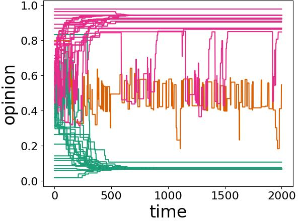
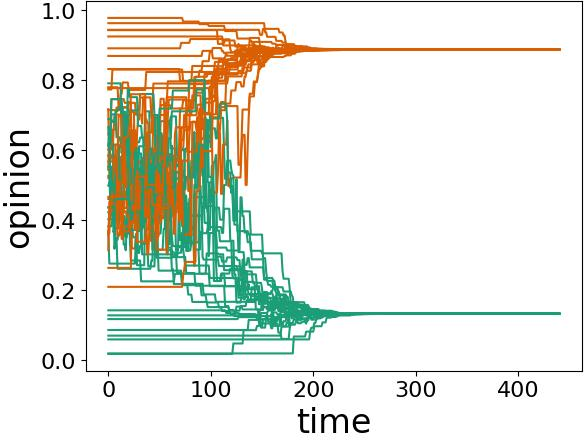
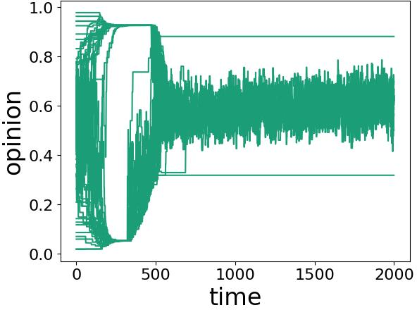
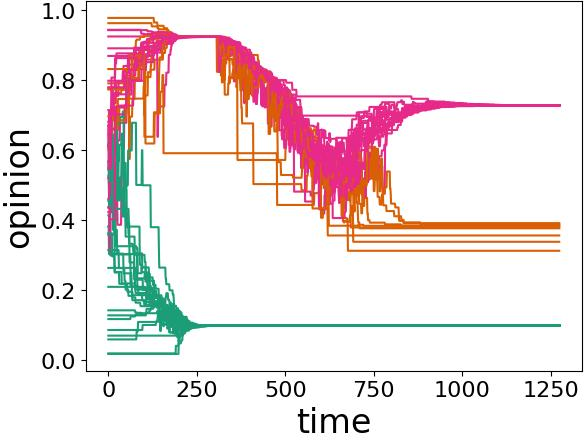
Figure 1: Several examples of opinion dynamics in our neighborhood DW (NDW) model with homophilic rewiring. In each panel, we show one simulation on a network. The neighborhood-tuning parameter \(\sigma\), the confidence bound \(\epsilon\), and the discordance threshold have the values (a) \(\sigma = 0\), \(\epsilon = 0.1\), and \(\zeta = 0.4\); (b) \(\sigma = 0.1\), \(\epsilon = 0.2\), and \(\zeta = 0.2\); (c) \(\sigma = 0\), \(\epsilon = 0.2\), and \(\zeta = 0.4\); and (d) \(\sigma = 0.1\), \(\epsilon = 0.1\), and \(\zeta = 0.3\). At each discrete time, we consider \(f = 0.2 N\) dyads, where \(N = 100\) is the size (i.e., the number of nodes) of the network. The convergence parameter is \(\rho = 0.3\). We choose edges uniformly at random; if an edge is discordant, we rewire it using the homophilic rewiring strategy 6 . It is possible for the same node to rewire multiple times. We initialize the network to be a \(G(N,p)\) Erdős–Rényi (ER) graph with an independent, homogeneous probability \(p = 0.3\) of an edge between each pair of nodes. We initialize each node opinion to a uniformly random value in the interval \([0,1]\). All depicted simulations use the same initial network and the same set of initial opinions. We terminate a simulation either when it reaches our stopping criterion or when \(t_{\text{max}} = 2000\) time steps have elapsed (whichever occurs first). We color the opinion trajectories of each node according to its opinion value at the end of a simulation. Any two nodes whose opinions differ by at least the confidence bound \(\epsilon\) are in different colors..
In Fig. 1, we show examples of various behaviors in our NDW model 3 . We color opinions according to their final opinion clusters. In each simulation, we initialize a network to be a \(G(N,p)\) Erdős–Rényi (ER) graph with \(N = 100\) nodes and an independent, homogeneous probability \(p = 0.3\) of an edge between each pair of nodes. We initialize the node opinions uniformly at random in the interval \([0,1]\). In each discrete time, we repeat a three-step process on \(f = nN\) distinct edges (as before, we take \(f = \lceil nN \rceil\) if \(nN\) is not an integer), which we choose uniformly at random without replacement. For each selected edge, we update the opinions of the incident nodes according to the opinion-update rule 3 . If the edge is discordant, we rewire it using one of the strategies in Section 4. (In Fig. 1, we use the homophilic rewiring strategy 6 .) We end a simulation either when it satisfies a stopping criterion or after \(t_{\text{max}} = 2000\) time steps (whichever occurs first). Our stopping criterion is that no node changes its opinion by more than \(10^{-3}\) in any time step for 200 consecutive time steps.
In Fig. 1 (a), we show a fragmented state with pseudo-consensus in the pink opinion cluster (top) and green opinion cluster (bottom). The orange opinion cluster (middle) has not converged after 2000 time steps. We observe opinion jumping at approximately times \(600\) and \(1900\); some opinion values (in pink) change by more than the confidence bound \(\epsilon\) in a single time step. In Fig. 1 (b), we show an example of polarization. In this simulation, there are also several opinion crossings. In Fig. 1 (c), two opinion clusters have converged (to opinions with values of approximately \(0.9\) and \(0.3\)) and one opinion cluster has not converged after 2000 time steps. The opinions in this last cluster oscillate wildly between values of about \(0.45\) and \(0.75\). In Fig. 1 (d), we observe a variety of interesting behaviors. These behaviors include fragmentation into three opinion clusters, pseudo-consensus in the orange opinion cluster (middle), consensus in the pink (top) and green (bottom) clusters, opinion crossing (which is most visible at early times), and opinion jumping (which is most visible in orange). Additionally, the pink opinion cluster has a temporary consensus between the approximate times \(250\) and \(350\).
5.2 Network dynamics through opinion-driven adaptation↩︎
In our adaptive NDW model, the structure of a network can change at each discrete time. These structural changes, in turn, affect the opinion dynamics on the network. In Fig. 2, we show the time evolution of the network properties in an adaptive network with homophilic rewiring 6 . We compare our NDW model to a baseline DW model for different values of the neighborhood-tuning parameter \(\sigma \in [0,1]\), where \(\sigma = 1\) corresponds to standard DW opinion updates and rewiring that depends only on dyadic homophily and \(\sigma = 0\) corresponds to pure NDW opinion updates and rewiring that depends only on transitive homophily. As we will illustrate, the network properties depend in an interesting way on \(\sigma\). We initialize the network to be a \(G(N,p)\) ER graph with \(N = 50\) nodes and an independent, homogeneous probability \(p = 0.3\) of an edge between each pair of nodes, and we initialize the node opinions uniformly at random in \([0,1]\). We indicate the other parameter values in the caption of Fig. 2. Each plot is a mean of 20 simulations with the same parameter values but different randomizations, including both different ER graphs and different sets of initial opinions, with standard errors indicated by the shaded regions.
In Fig. 2 (a), we plot the time evolution of the number of discordant edges. We observe a marked difference between the baseline DW model, in which the number of discordant edges decreases almost monotonically as a function of time, and the pure NDW model, in which the number of discordant edges tends to increase early in simulations (after a small initial dip) and subsequently decreases almost monotonically. In Fig. 2 (b), we show the time evolution of the spectral gap of the adjacency matrix \(A\). The spectral gap is the absolute value of the difference between the two largest eigenvalues of \(A\). For a time-independent network, the spectral gap is inversely proportional to the relaxation time of the mixing of a standard random walk on a network [52], [53]. Notably, the behavior of the NDW model with \(\sigma = 0.5\), which assigns equal importance to the distances from the NDW and DW models, does not linearly interpolate between the two extreme cases. In Fig. 2 (c), we plot the time evolution of the degree-assortativity coefficient, which is equal to the Pearson correlation coefficient of the node degrees between pairs of neighboring nodes [54]. Positive values of assortativity indicate a positive correlation between nodes of similar degrees. We observe that assortativity tends to increase with time for all cases, as expected for homophilic rewiring. However, it appears to saturate for the pure NDW model (i.e., when \(\sigma = 0\)). It is also much smaller for the pure NDW model than for the other examined situations.
In Fig. 2 (d), we plot the time evolution of the fraction of the \(f\) chosen edges in a time step that we rewire due to discordance. Recall that we consider \(f\) edges (i.e., \(f\) dyads) at each discrete time, but we only rewire the discordant edges. We observe a pattern that resembles the one in Fig. 2 (a), although Fig. 2 (d) is much noisier. In Fig. 2 (e), we examine the time evolution of the fraction of the nodes in the chosen dyads that update their opinions. It is sensible but still worth remarking that the fraction of edges that are discordant is not inversely correlated with the fraction of opinion updates. Edge discordance and opinion updates are governed by different parameters. Interestingly, although the pure NDW model initially has the fewest opinion updates, it eventually has the most opinion updates. It is also relevant to compare the total amount by which opinions change for different values of the neighborhood-tuning parameter \(\sigma\). We consider \(\sigma \in \{0,0.5,1\}\) and observe noticeable differences in dynamics for the different values of \(\sigma\).
In Fig. 2 (f), we plot the time evolution of the mean number of connected components of the networks. The pure NDW model our baseline DW model both typically yield the same mean number of connected components (usually \(1\)), although the pure NDW model eventually produces more components than the baseline DW model. Interestingly, we eventually obtain the largest mean number of connected components for \(\sigma = 0.5\), which uses a mixture of the NDW and standard DW opinion-update rules.
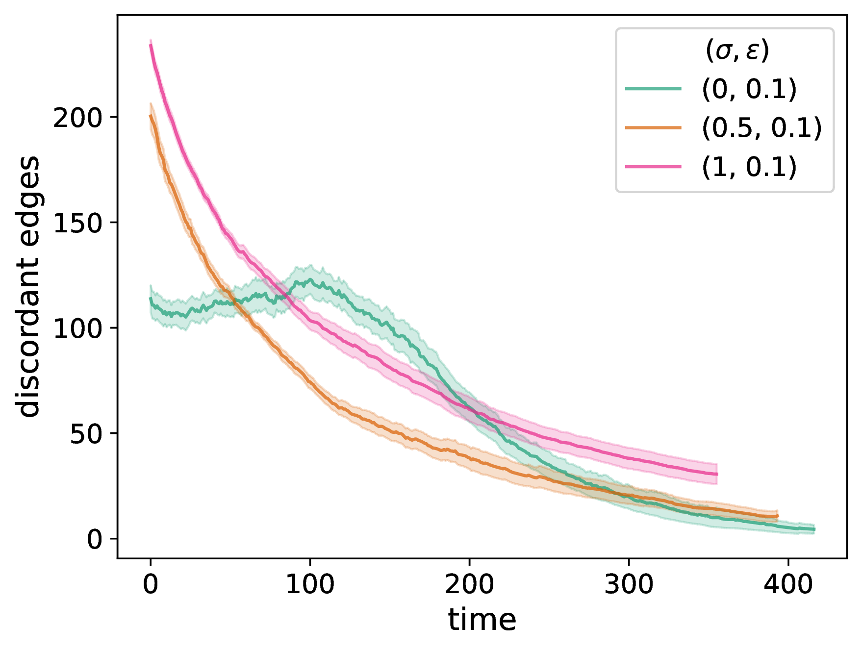
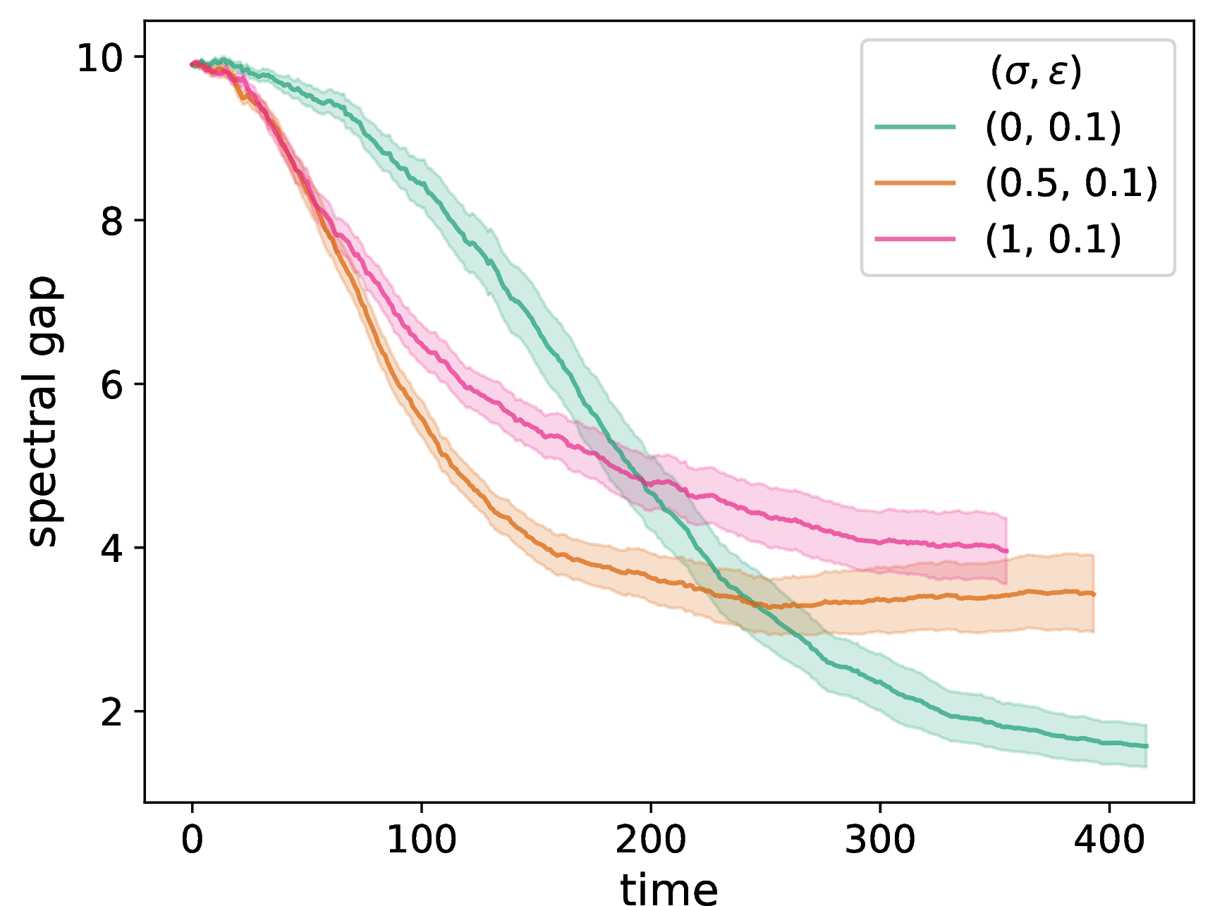
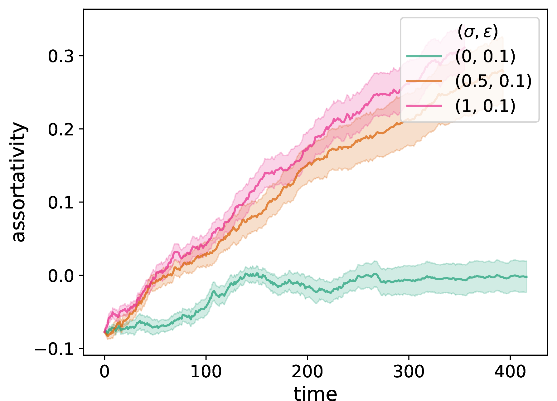
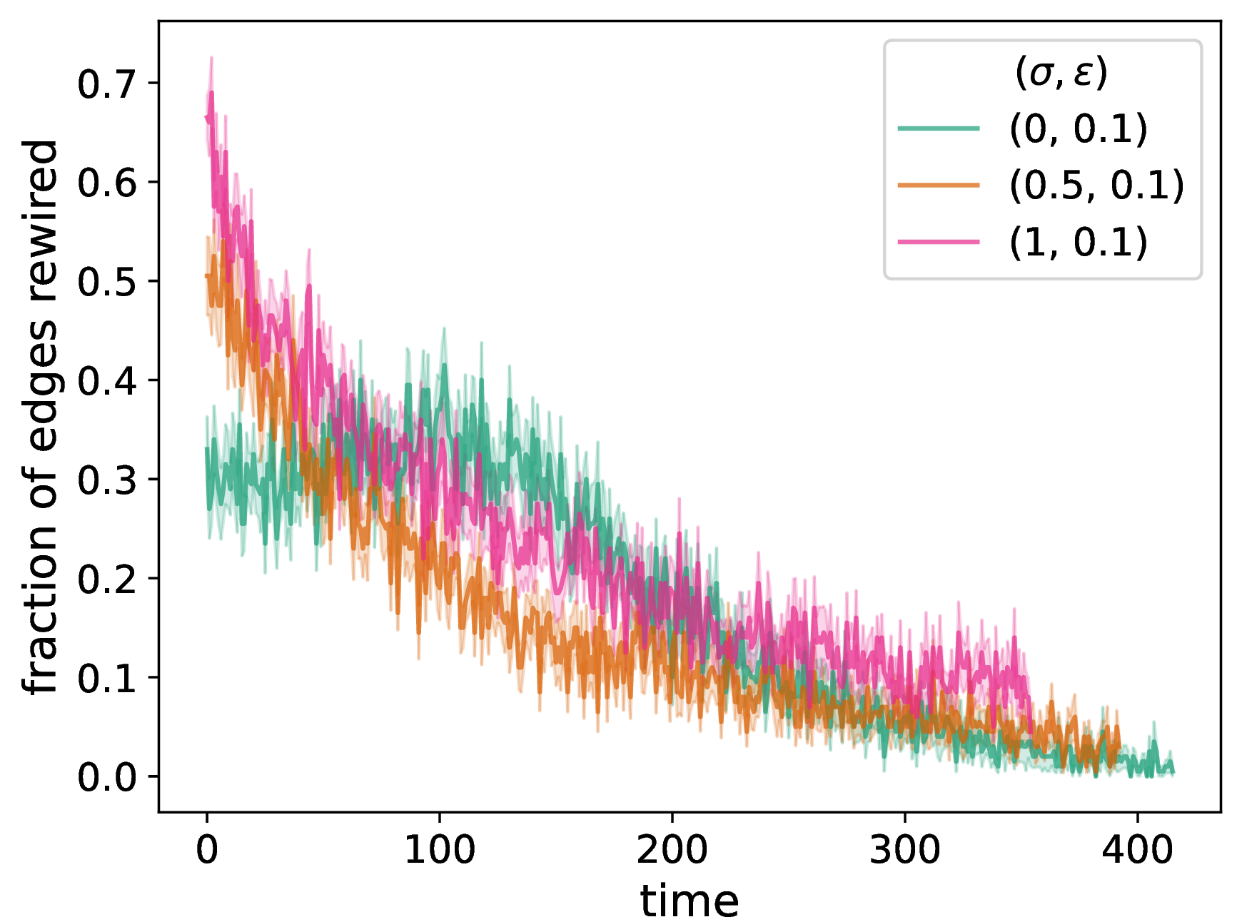
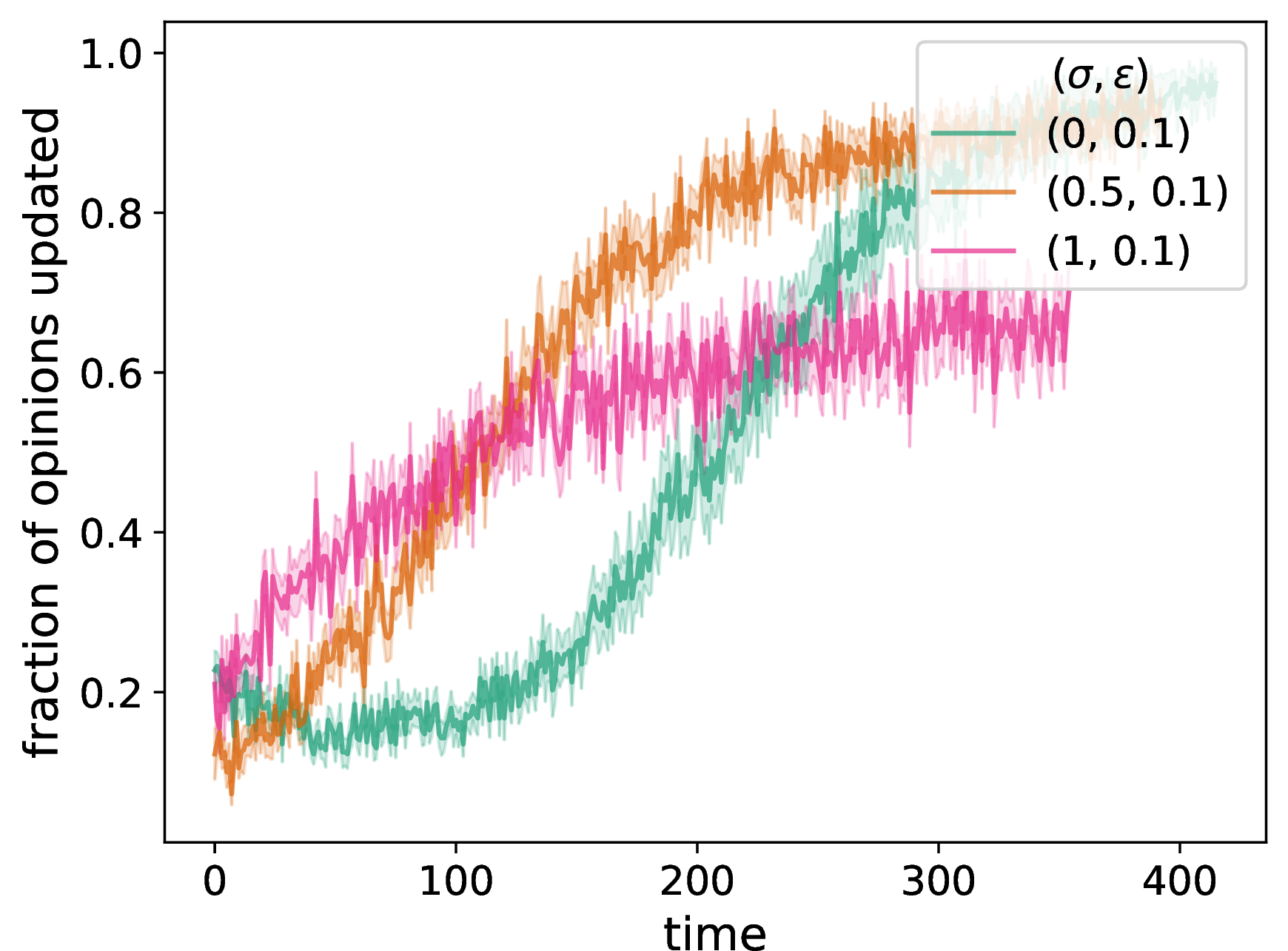
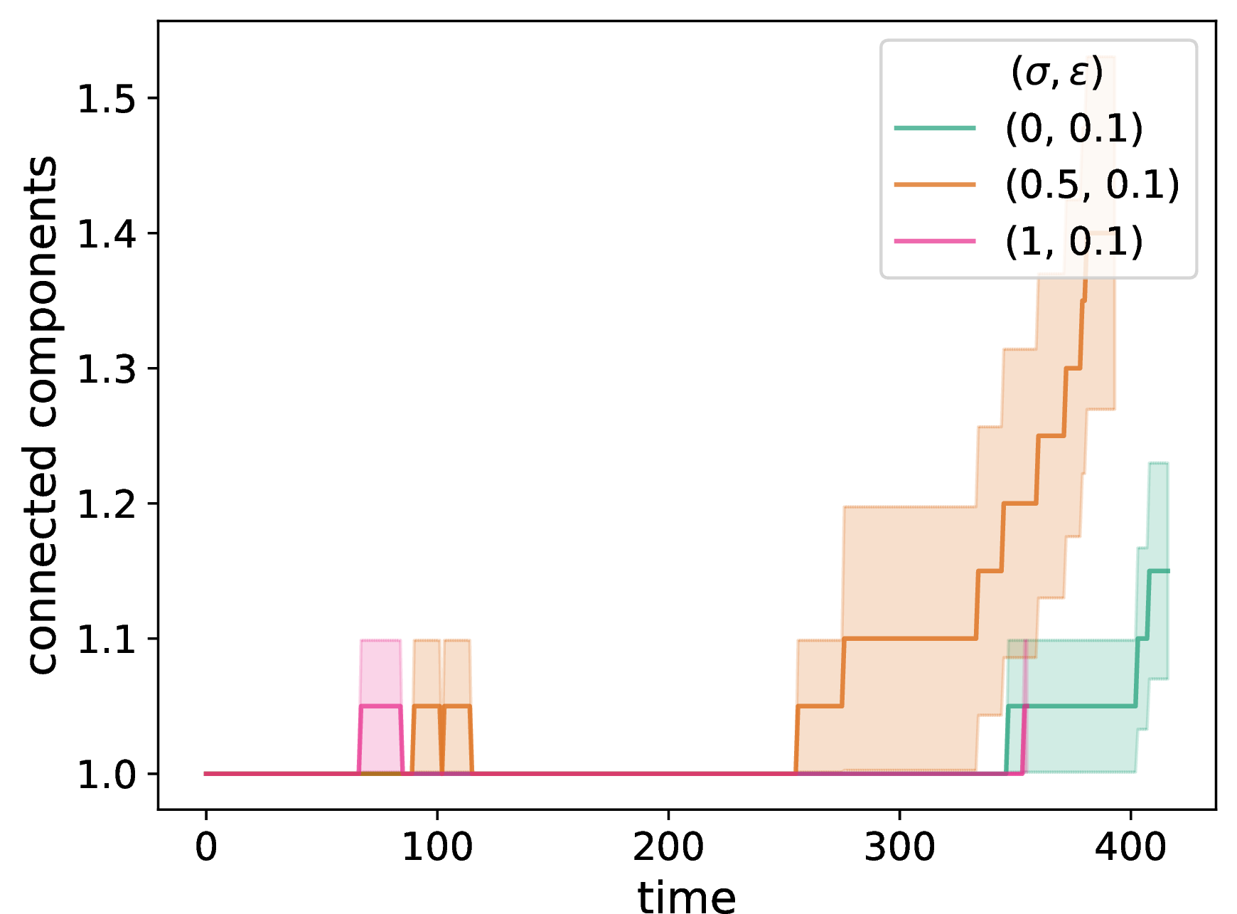
Figure 2: We examine network adaptation as a function of time in our NDW model by plotting (a) the number of discordant edges in the network, (b) the spectral gap of the adjacency matrix, (c) a degree-assortativity coefficient, (d) the fraction of edges in the chosen dyads that rewire (i.e., that are discordant), (e) the fraction of nodes in the chosen dyads that update their opinion, and (f) the mean number of connected components of the networks. We compare the network properties for a pure DW opinion-update rule (i.e., \(\sigma = 1\)), a mixed DW and NDW opinion-update rule with \(\sigma = 0.5\), and a pure NDW opinion-update rule (i.e., \(\sigma = 0\)). We initialize each network to be a \(G(N,p)\) ER network with \(N = 50\) nodes and an independent, homogeneous probability \(p = 0.3\) of an edge between each pair of nodes. For each network, we initialize each node opinion to a uniformly random value in \([0,1]\). We plot means of 20 simulations, with the same 20 initial networks and sets of initial opinions for each curve and each panel. The shaded regions indicate the standard error. The confidence bound is \(\epsilon = 0.1\), the discordance threshold is \(\zeta = 0.2\), the number of chosen edges at each discrete time for interaction is \(f = 0.2 N\), and the convergence parameter is \(\rho = 0.3\). We terminate a simulation either when it reaches our stopping criterion or when \(t_{\text{max}} = 2000\) time steps have elapsed (whichever occurs first)..
6 A multilayer model of coevolving opinions and diseases↩︎
The study of diseases and how they spread is (of course) extremely important, and it is essential to consider the interplay between human behavior and disease spread [38], [39], [42]. We investigate the effects of our NDW model with network adaptation on disease spread by combining opinion dynamics and disease dynamics in a two-layer opinion–disease model. We place our NDW model on one layer and a compartmental disease-spread model on the other layer. We couple these models through an adaptive contact network, on which the opinions change and the disease spreads. The network adaptation itself can occur both through changes in both opinion states (e.g., through homophilic rewiring) or through changes in disease states (e.g., quarantining of an infected agent).
Suppose that the agents of a network are connected in a graph \(G = (V,E)\) with a time-independent set \(V\) of nodes and a time-dependent set \(E = E(t) \subset V \times V\) of edges. The corresponding adjacency matrix at time \(t\) is \(A(t)\). The contact network \(G\) is shared by both layers; its structure can change at each discrete time both through changes in opinions and through changes in disease states. Each time step has a four-step process:
Opinion spreading: We use our NDW model (see Section 3) of opinion dynamics. We select \(f = nN\) edges uniformly at random without replacement and update the opinions of the associated nodes using Eq. 3 .
Opinion-driven network rewiring: If a chosen edge is discordant, we rewire it. The rewiring (see Section 4), which changes the structure of \(G\), can be uniformly at random or homophilic [see Eq. 6 ].
Disease spreading: We simulate one instantiation of a disease-spread model on the new network. We use an SIR model, but one can alternatively consider other models of disease spread. See Section 6.1 for more details about the disease dynamics.
Disease-driven network rewiring: The network structure changes as a result of disease-driven network adaption. We remove edges from newly infected nodes and add edges to newly recovered nodes. The rewiring can be uniformly at random or homophilic. See Section 6.2 for more details of the disease-driven rewiring.
We outline our four-step process in Algorithm 1. In the subsections below, we describe step [step323] (which specifies the disease dynamics) and step [step324] (which specifies disease-driven network adaptation) in detail. We think of each edge as representing an in-person contact between two agents. A change in these contacts affects both the opinion dynamics and the disease dynamics. For example, if neighboring agents disagree strongly with each other and sever the edge between them, they cannot subsequently spread an infectious disease to each other unless they reestablish the edge. Additionally, the isolation of an infected agent severs many of their edges to other agents, so they no longer have these in-person contacts to influence other agents or be influenced by them. In practice, isolated agents can certainly share their opinions online, but we are assuming for simplicity that both layers have the same network structure and that edges capture only in-person interactions. It is, of course, interesting to generalize our multilayer model to consider different network structures in the two layers.
6.1 Disease-spread model↩︎
We model the spread of an infectious disease using an SIR compartmental model, which is studied commonly on networks [47], [55], including on adaptive networks [32].
At each discrete time, each node of a network is in the susceptible (S), infected (I), or recovered (R) compartment (i.e., disease state). In our simulations, we choose 5% of the nodes uniformly at random to start in compartment I. All other nodes are initially in compartment S. If there is an edge between a susceptible node and an infected node, at each discrete time, the susceptible node is infected through that contact with transmission probability \(\beta\). Additionally, at each time, an infected node recovers spontaneously (and hence moves to compartment R) with recovery probability \(\gamma\). There are no other possible transitions between compartments. Recovered nodes are immune to the disease, so they cannot be reinfected.
6.2 Disease-driven network adaptation↩︎
In an SIR model, the disease states (i.e., compartments) of agents can change in two ways. Agents in compartment S can become infected and move to compartment I, and agents in compartment I can recover and move to compartment R. The network structure changes (i.e., there is disease-driven network adaptation) when agents change compartments.
When an individual becomes infected (i.e., moves from compartment S to compartment I), we expect them to interact less with other individuals. The removal of such in-person contacts can arise from a quarantine, caution, reduction in social activity, or something else [56]. In our simulations, we suppose that a newly infected node removes \(m\) edges to susceptible nodes to reduce the risk of spreading the disease. As we describe below, we choose susceptible nodes to which to remove an edge either uniformly at random or in a way that depends on node opinions and neighborhood opinions [see Eq. 7 ]. If the newly infected node has fewer than \(m\) contacts to susceptible nodes, then it removes all such contacts. Because recovered nodes have permanent immunity and infected nodes are already infected, we assume that infected nodes do not change their interactions with recovered or infected nodes. An interesting alternative scenario to consider is a newly infected node removing contacts with some fraction of its contacts, irrespective of their compartments. In our model, it is only newly infected nodes that sever connections; in particular, a susceptible node does not take initiative to remove a connection to an infected node.
When a node recovers (i.e., moves from compartment I to compartment R), it resumes interacting with susceptible and recovered nodes. To do this, it adds contacts to \(m\) nodes (either uniformly at random or following a homophilic strategy) to susceptible and recovered nodes, with the nodes in the two compartments treated on equal footing. We attach a total of \(m\) edges from the newly recovered nodes to nodes in compartments S or R. The newly recovered nodes do not attach to infected nodes.
We now describe the network adaptation mathematically. At each discrete time \(t\), nodes can stay in the same compartment, move from compartment S to compartment I, or move from compartment I to compartment R. Let \(y_i(t) \in \{\text{S}, \text{I}, \text{R}\}\) be the disease state of node \(i\) at time \(t\). Network adaptation on the disease layer occurs in two ways:
Removal of edges: Consider a node \(i\) that becomes infected at time \(t\) (i.e., \(y_i(t - 1) = \text{S}\) and \(y_i(t) = \text{I}\)). Consider the set \(Z_i\) of nodes that are adjacent to node \(i\) and susceptible at time \(t\). Choose \(m\) nodes by removing — either uniformly at random or in a way that preferentially removes nodes with different opinions and different neighborhood opinions [see Eq. 7 ] — edges from nodes \(j \in Z_i\) to these \(m\) nodes.
Addition of edges: Consider a node \(i\) that recovers at time \(t\) (i.e., \(y_i(t - 1) = \text{I}\) and \(y_i(t) = \text{R}\)). Consider the set \(Y_i\) of nodes that are not adjacent to node \(i\) and are either susceptible or recovered at time \(t\). Choose \(m\) nodes by adding — either uniformly at random or homophilically 8 — edges to nodes \(j \in Y_i\).
In our coupled opinion–disease model, the disease-driven network adaptation can depend on node opinions through homophilic adaptation. For instance, a newly recovered node may choose to connect preferentially to nodes with opinions that are similar to its opinion (through dyadic homophily) or to nodes whose mean neighbor opinion is similar to its opinion (through transitive homophily). Analogously, a newly infected individual may choose to sever connections preferentially from nodes whose opinions are dissimilar to its opinion (through dyadic homophily) or from nodes whose mean neighbor opinion is similar to its opinion (through transitive homophily). Additionally, edge removal and addition due to a change in a disease state models situations, such as quarantining and re-entry into society, that change a contact network, thereby affecting the ability of nodes to affect the opinions of others.
We consider two different rewiring strategies for choosing the probability distributions for addition and removal of edges. These strategies are as follows:
Random rewiring: A node \(i\) that has just entered a new disease state chooses \(m\) nodes from the set of nodes in allowed compartments uniformly at random to break an edge from (for edge removal) or add an edge to (for edge addition). When a node becomes infected, the allowed compartment is S; when a node recovers, the allowed compartments are S and R.
Homophilic rewiring: In the removal of edges, a newly infected node \(i\) breaks an edge from a node \(j \in Z_i\) with probability \[P(i \not \to j) = \frac{\sigma d_{\text{BC}}(i,j) + (1 - \sigma) d_{\text{NBC}}(j,i)}{\sum_j (\sigma d_{\text{BC}}(i,j) + (1 - \sigma) d_{\text{NBC}}(j,i))} \,, \label{eq:rewire95SI}\tag{7}\] where \(\sigma\) is the neighorhood-tuning parameter. The newly infected node is more likely to break edges from nodes whose opinions are dissimilar to its opinion and from nodes whose mean neighbor opinion is dissimilar to its opinion.
Analogously, in the addition of edges, a newly recovered node \(i\) forms an edge to a node \(j \in Y_i\) with probability \[P(i \to j) = \frac{1 - (\sigma d_{\text{BC}}(i,j) + (1 - \sigma) d_{\text{NBC}}(j,i))}{\sum_j (1 - (\sigma d_{\text{BC}}(i,j) + (1 - \sigma) d_{\text{NBC}}(j,i)))} \,. \label{eq:rewire95IR}\tag{8}\] The newly recovered node is more likely to add edges to nodes whose opinions are similar to its opinion and to nodes whose mean neighbor opinion is similar to its opinion.
For both removing and adding connections, the homophilic disease-driven rewiring captures a notion of transitive homophily. It resembles the homophilic opinion-driven rewiring strategies in Section 4. The edge-addition strategy is the same in both types of rewiring.
None
Figure 3: No caption
7 Numerical simulations of our two-layer opinion–disease model↩︎
We now present the results of numerical simulations of our multilayer opinion–disease model. We discuss results for network dynamics, opinion dynamics, and disease dynamics.
7.1 Network dynamics in our multilayer model↩︎
At each discrete time, the network changes twice. As outlined in Section 6, it first changes through opinion-driven rewiring (see step [step322] of a time step) and it then changes through disease-driven rewiring (see step [step324]). We examine how several properties of the network structure evolve with time.
In Fig. 4, we show the time evolution of several network properties in our two-layer opinion–disease model with homophilic adaptation in both the disease layer and the opinion layer. We use our NDW model on the opinion layer and an SIR compartmental model on the disease layer. We initialize the network to be a \(G(N,p)\) ER graph with \(N = 50\) nodes and an independent, homogeneous probability \(p = 0.3\) of an edge between each pair of nodes. We initialize opinions to uniformly random values in the interval \([0,1]\). (We specify the other parameters in the caption of Fig. 4.) We choose 5% of the nodes uniformly at random to be in the infected state; all other nodes start in the susceptible state. Each plot is a mean of 20 simulations with the same parameter values but different ER networks and a different set of initial opinions, with standard errors indicated by the shaded regions. We examine various network properties as a function of the neighborhood-tuning parameter \(\sigma \in [0,1]\) (with the other parameters fixed). By considering different values of \(\sigma\), we compare results for our pure NDW model, our baseline DW model, and a situation that interpolates between these two extreme cases.
In Fig. 4, we observe results that are very similar to those of our adaptive NDW model with homophilic adaptation but without disease dynamics (see Fig. 2). The most noticeable difference arises in our plot of the time evolution degree assortativity; see Figs. 2 and 4. For the multilayer opinion–disease model [see Fig. 4 (c)], the case \(\sigma = 0.5\) seems interpolates roughly halfway between the two extreme cases (i.e., the pure NDW model and our baseline DW model). By contrast, for the opinion-only model [see Fig. 2 (c)], the \(\sigma = 0.5\) curve is much closer to the NDW curve than to the baseline DW curve. In the multilayer opinion–disease model, we also observe (as in the opinion-only model) that transitive homophily results in interesting and nontrivial dependence of network structure on \(\sigma\), with \(\sigma = 0.5\) often yielding qualitatively different curves than \(\sigma \in \{0,1\}\).
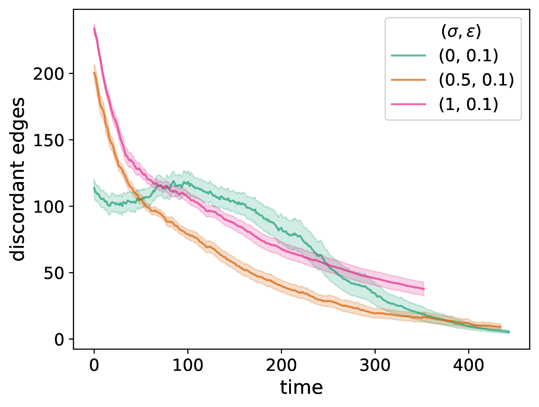
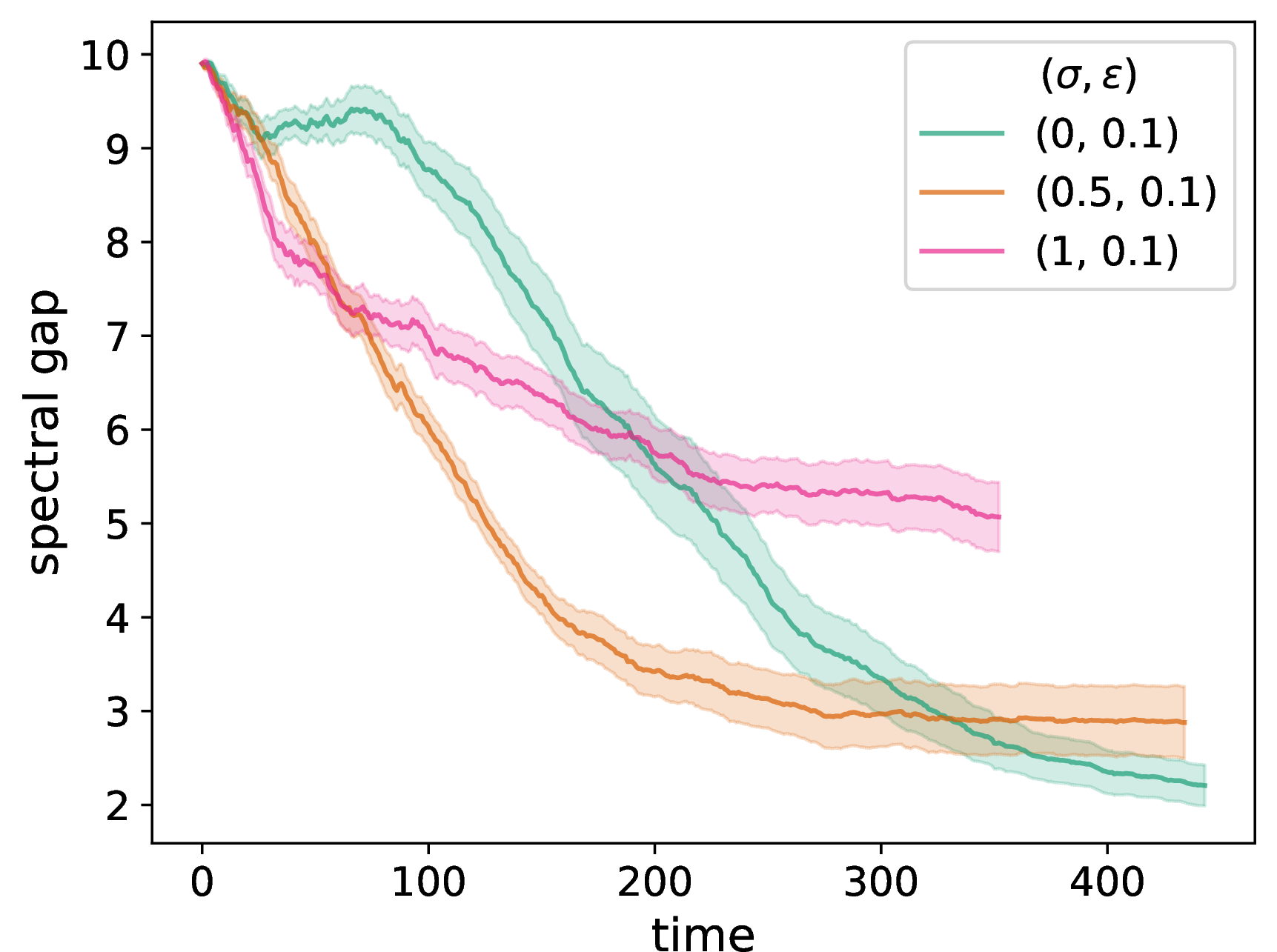
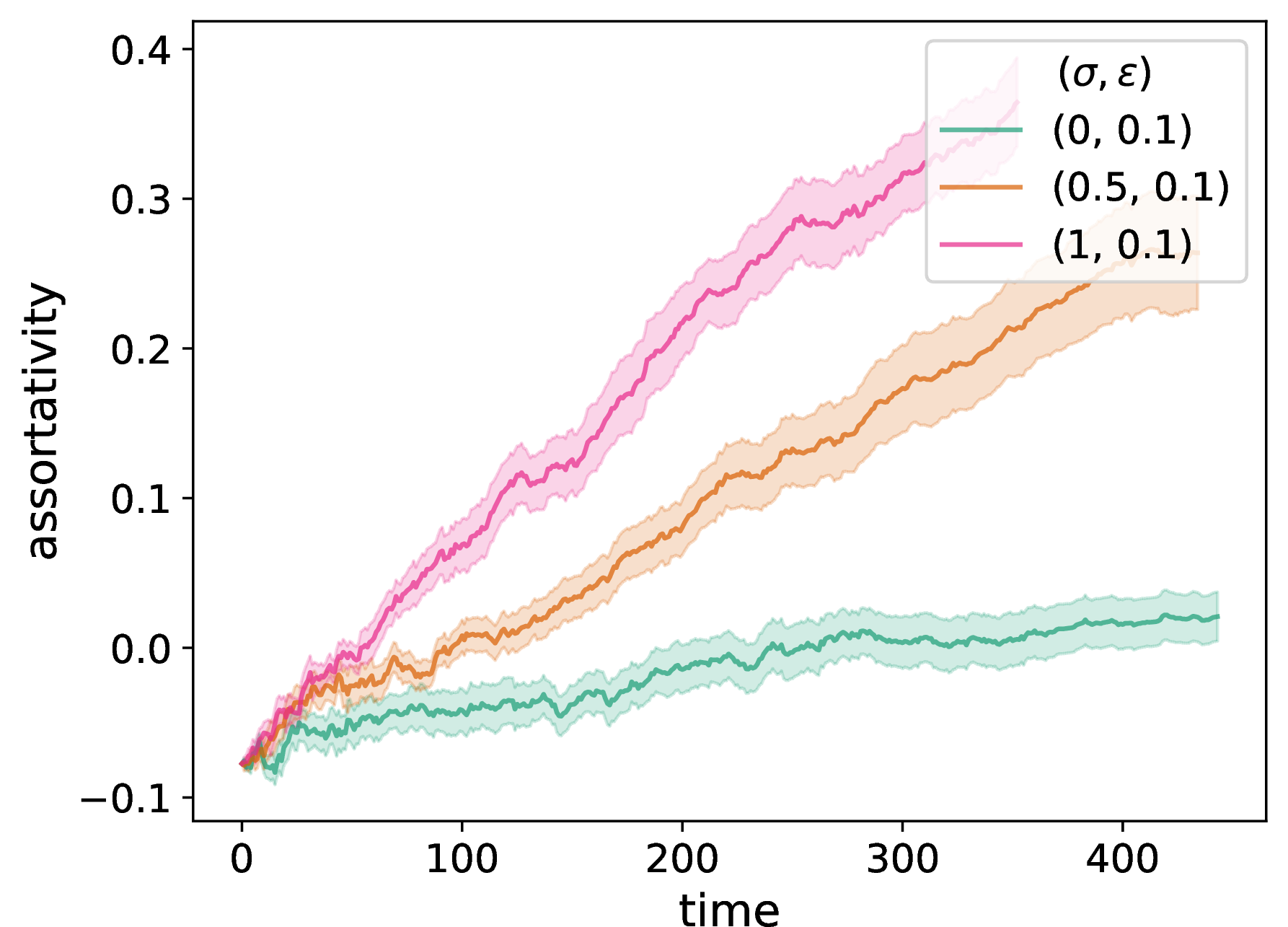
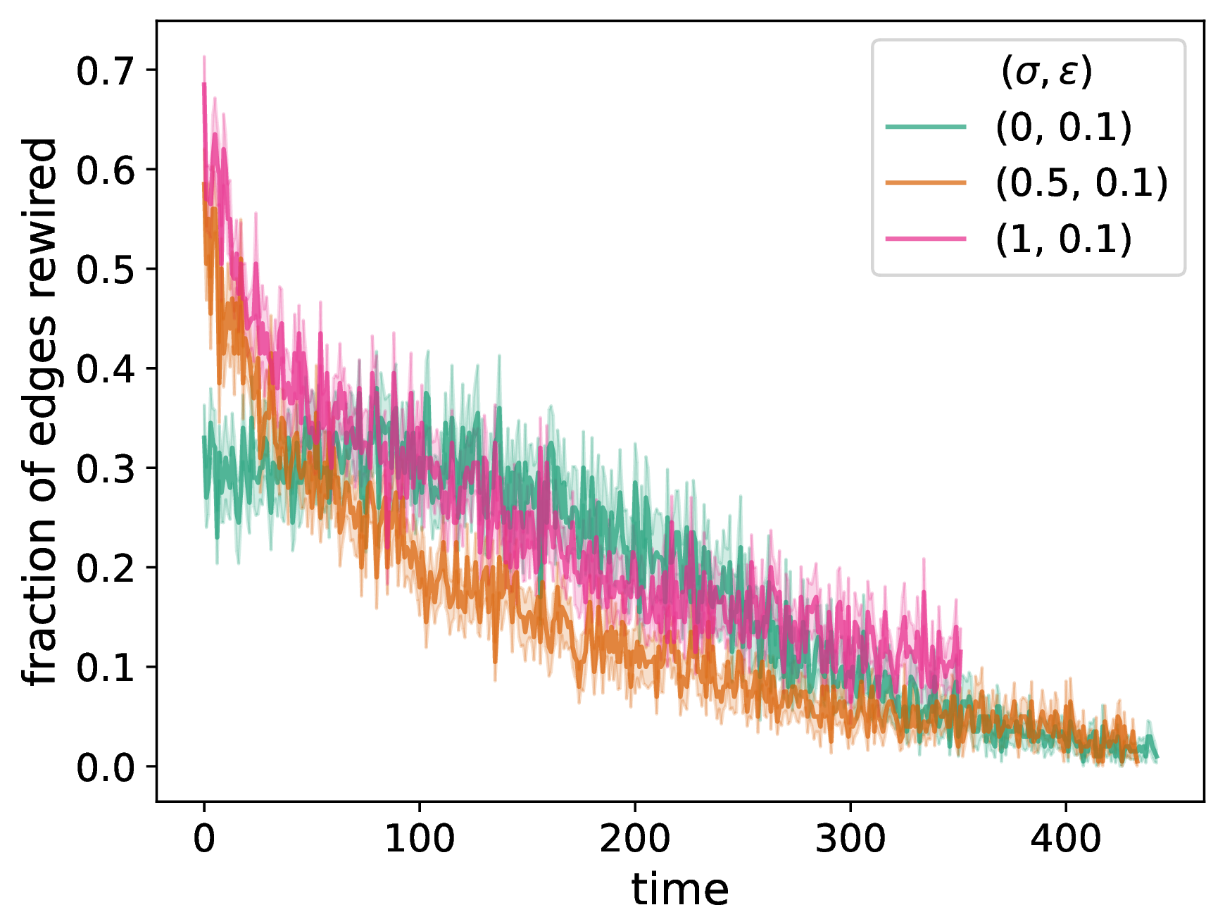
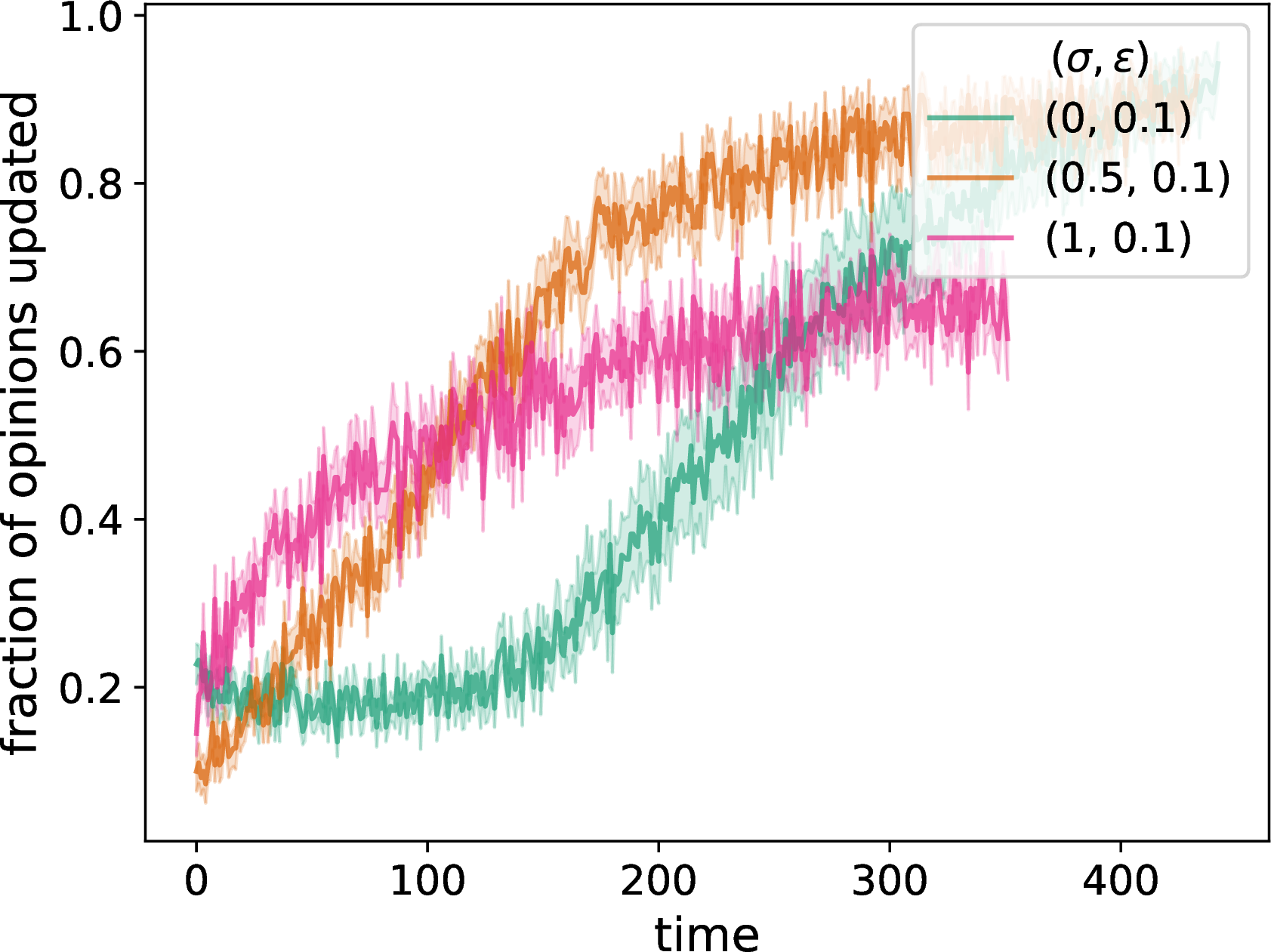
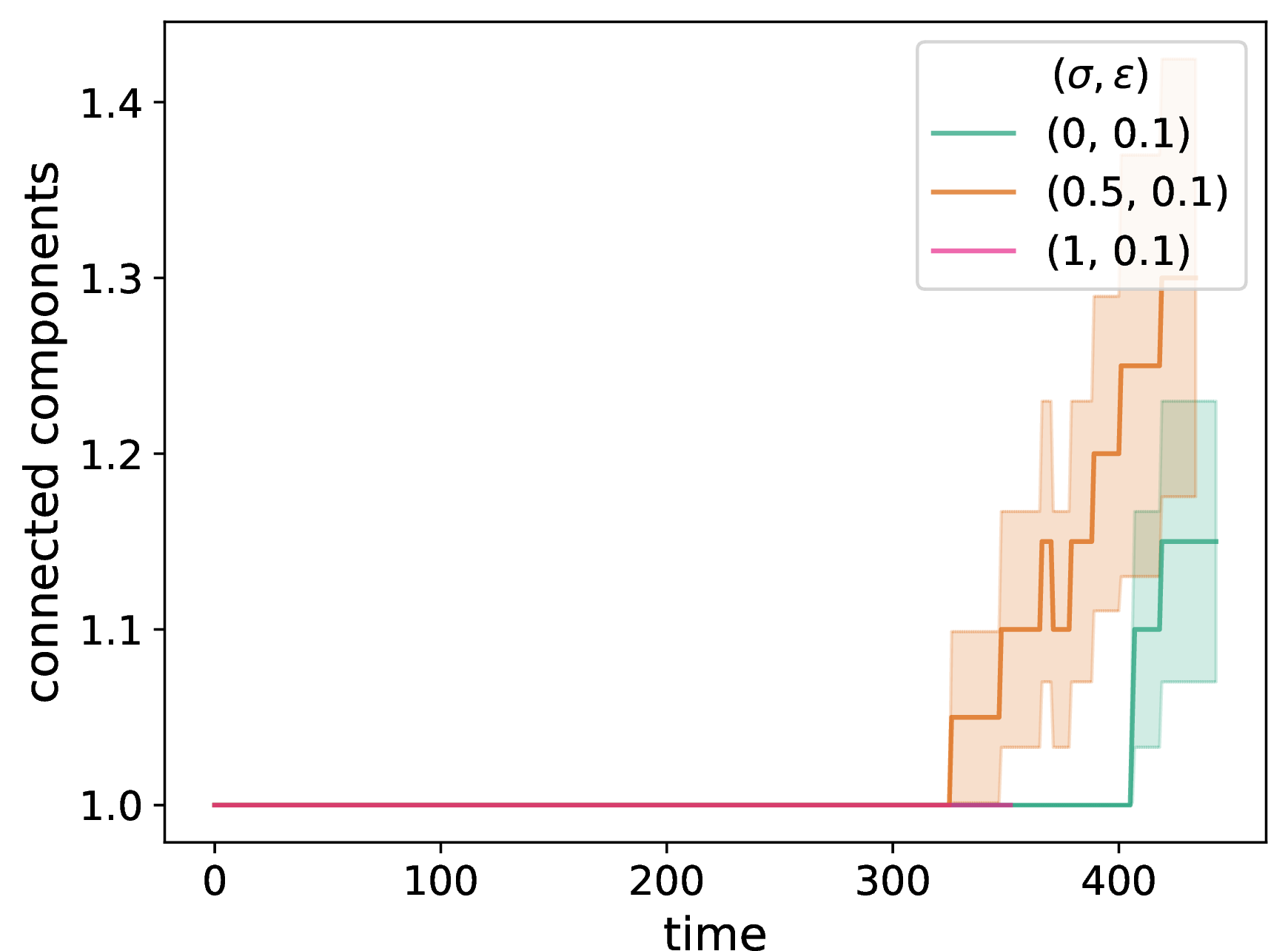
Figure 4: We examine the time evolution of network structure in our opinion–disease multilayer model by plotting (a) the number of discordant edges in the network, (b) the spectral gap of the adjacency matrix, (c) a degree-assortativity coefficient, (d) the fraction of edges in the chosen dyads that rewire (i.e., that are discordant), (e) the fraction of nodes in the chosen dyads that update their opinion, and (f) the number of connected components of the network. We compare the properties of adaptive networks for a pure DW opinion-update rule (i.e., \(\sigma = 1\)), a mixed DW and NDW opinion-update rule with \(\sigma = 0.5\), and a pure NDW opinion-update rule (i.e., \(\sigma = 0\)). We consider an SIR compartmental model on the disease layer. We initialize each network to be a \(G(N,p)\) ER graph with \(N = 50\) nodes and an independent, homogeneous probability \(p = 0.3\) of an edge between each pair of nodes. For each network, we initialize each node opinion to a uniformly random value in \([0,1]\). We plot means of 20 simulations, with the same 20 initial networks and sets of initial opinions for each curve and each panel. The shaded regions indicate the standard error. The confidence bound is \(\epsilon = 0.1\), the discordance threshold is \(\zeta = 0.2\), and the convergence parameter \(\rho = 0.3\). We consider \(f = 0.2 N\) edges at each discrete time for opinion comparisons. The SIR model has a transmission probability of \(\beta = 0.01\) and a recovery probability of \(\gamma = 0.05\). In the disease layer, we update a network using homophilic disease-induced adaptation (see Section 6.2). Whenever a node enters compartment I, we remove \(m = 0.1 N\) of its edges; whenever a node enters compartment R, we add \(m = 0.1 N\) edges. For each network, we choose 5% of the nodes uniformly at random as initially infected; all other nodes are initially susceptible. We terminate a simulation either when it reaches our stopping criterion or when \(t_{\text{max}} = 2000\) time steps have elapsed (whichever occurs first). We plot means of 20 simulations, with the same 20 initial networks, sets of initial opinions, and sets of initially infected nodes for each curve and each panel. The shaded regions indicate the standard error..
7.2 Opinion dynamics in our multilayer model↩︎
We investigate how the coupling with disease dynamics affects opinion dynamics. In this discussion, all of our simulations reach our stopping criterion. We examine how the sizes of the largest and second-largest opinion clusters depend on the confidence bound \(\epsilon\) and the neighborhood-tuning parameter \(\sigma\). One way to quantify the opinion clusters in an opinion profile is by calculating the dispersion index [57] \[d = \frac{\sum_i s_i^2}{(\sum_i s_i)^2} \,,\] where \(s_i\) is the size of the \(i^{\text{th}}\) opinion cluster. An opinion profile with \(r\) equal-sized clusters yields \(d = 1/r\).
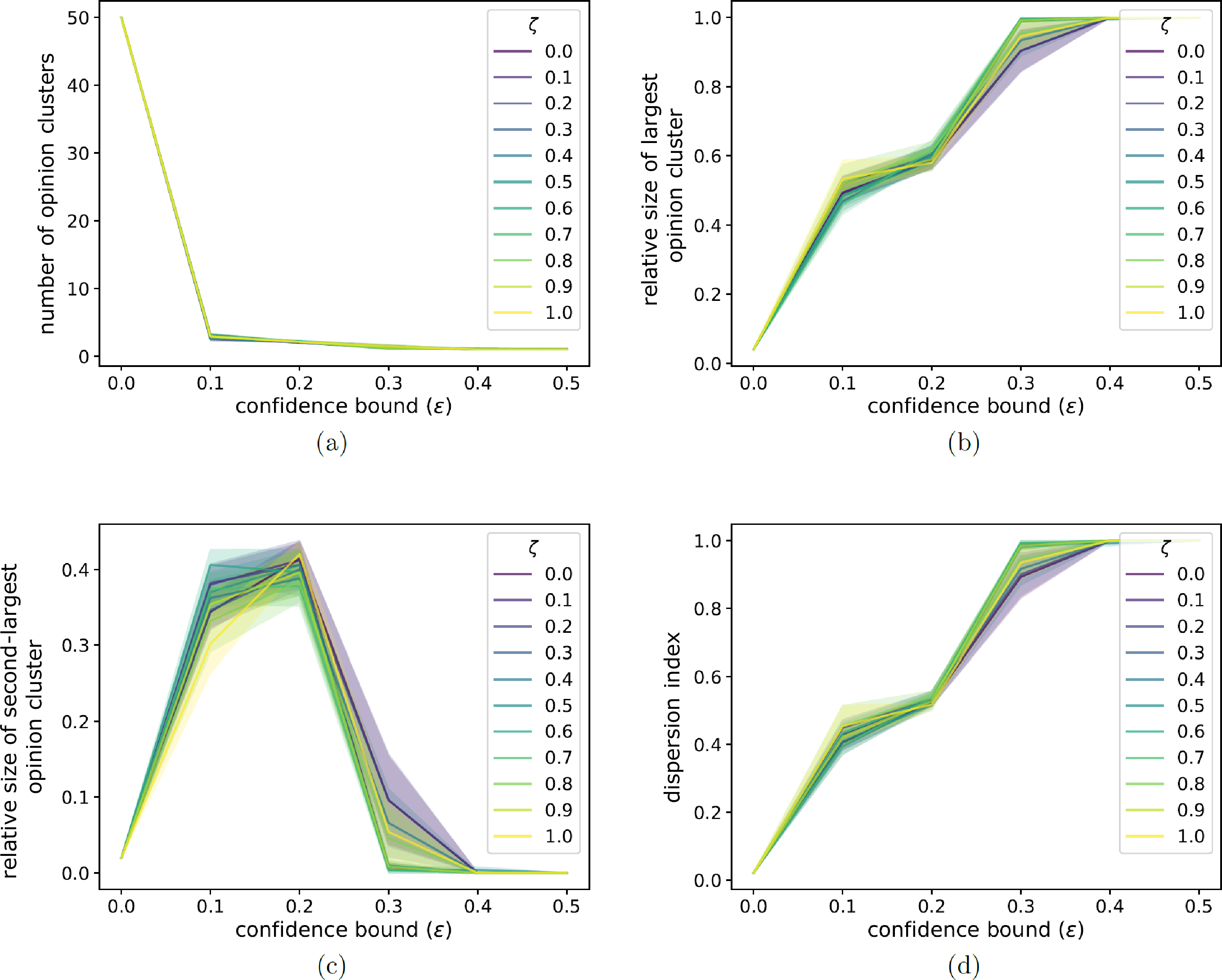
Figure 5: We illustrate the dependence of several final opinion-profile properties in our two-layer opinion–disease model on the confidence bound \(\epsilon\) for different values of the neighborhood-tuning parameter \(\sigma\). We show (a) the number of opinion clusters, (b) the fraction of nodes in the largest opinion cluster, (c) the fraction of nodes in the second-largest opinion cluster, and (d) the dispersion index \(d\). We initialize each network to be a \(G(N,p)\) ER graph with \(N = 50\) nodes and an independent, homogeneous probability \(p = 0.3\) of an edge between each pair of nodes. For each network, we initialize each node opinion to a uniformly random value in \([0,1]\). The discordance threshold is \(\zeta = 0.2\), the number of edges that we select at each discrete time for agents to interact is \(f = 0.2N\), and the convergence parameter is \(\rho = 0.3\). The SIR model has a transmission probability of \(\beta = 0.01\) and a recovery probability of \(\gamma = 0.05\). In the disease layer, we update a network using homophilic disease-induced adaptation (see Section 6.2). Whenever a node enters compartment I, we remove \(m = 0.1N\) of its edges; whenever a node enters compartment R, we add \(m = 0.1N\) edges. We choose 5% of the nodes uniformly at random as initially infected; all other nodes are initially susceptible. All depicted simulations reach our stopping criterion. We plot means of 20 simulations, with the same 20 initial networks, sets of initial opinions, and sets of initially infected nodes for each curve and each panel. The shaded regions indicate the standard error.
In Fig. 5, we show the dependence of several final opinion-profile properties on the confidence bound \(\epsilon\) for different values of the neighborhood-tuning parameter \(\sigma\). In Fig. 5 (a), we see that the number of opinion clusters tends to decrease rapidly as the confidence bound increases. It decreases drastically between \(\epsilon = 0\) and \(\epsilon = 0.1\). Additionally, for \(\epsilon = 0.1\), smaller \(\sigma\) (i.e., giving more weight to neighborhood effects) yields slightly fewer opinion clusters. In Figs. 5 (b,c), we show the relative sizes (with respect to the total number of nodes) of the largest and second-largest opinion clusters. The relative size of the largest opinion cluster tends to grow with \(\epsilon\) and appears to reach \(1\) for \(\epsilon \geq 0.4\) for all values of \(\sigma\). By contrast, the relative size of the second-largest cluster depends nonlinearly on \(\epsilon\), with a peak size at about \(\epsilon = 0.2\). For both the largest and second-largest clusters, the dependence on \(\epsilon\) appears to be smoother for large \(\sigma\) than for small \(\sigma\). Neither the dependence on \(\epsilon\) nor the dependence on \(\sigma\) is particularly intuitive, so they merit further exploration.
Based on the sizes of the top two opinion clusters [again see Figs. 5 (b,c)], there are additional (i.e., more than two) opinion clusters for many parameter values. In Fig. 5 (d), we observe that the dispersion index tends to increase with \(\epsilon\), with interesting trends for neighborhood effects (e.g., for \(\sigma < 0.5\)). The dispersion index appears to follow a similar trend as the size of the largest opinion cluster.
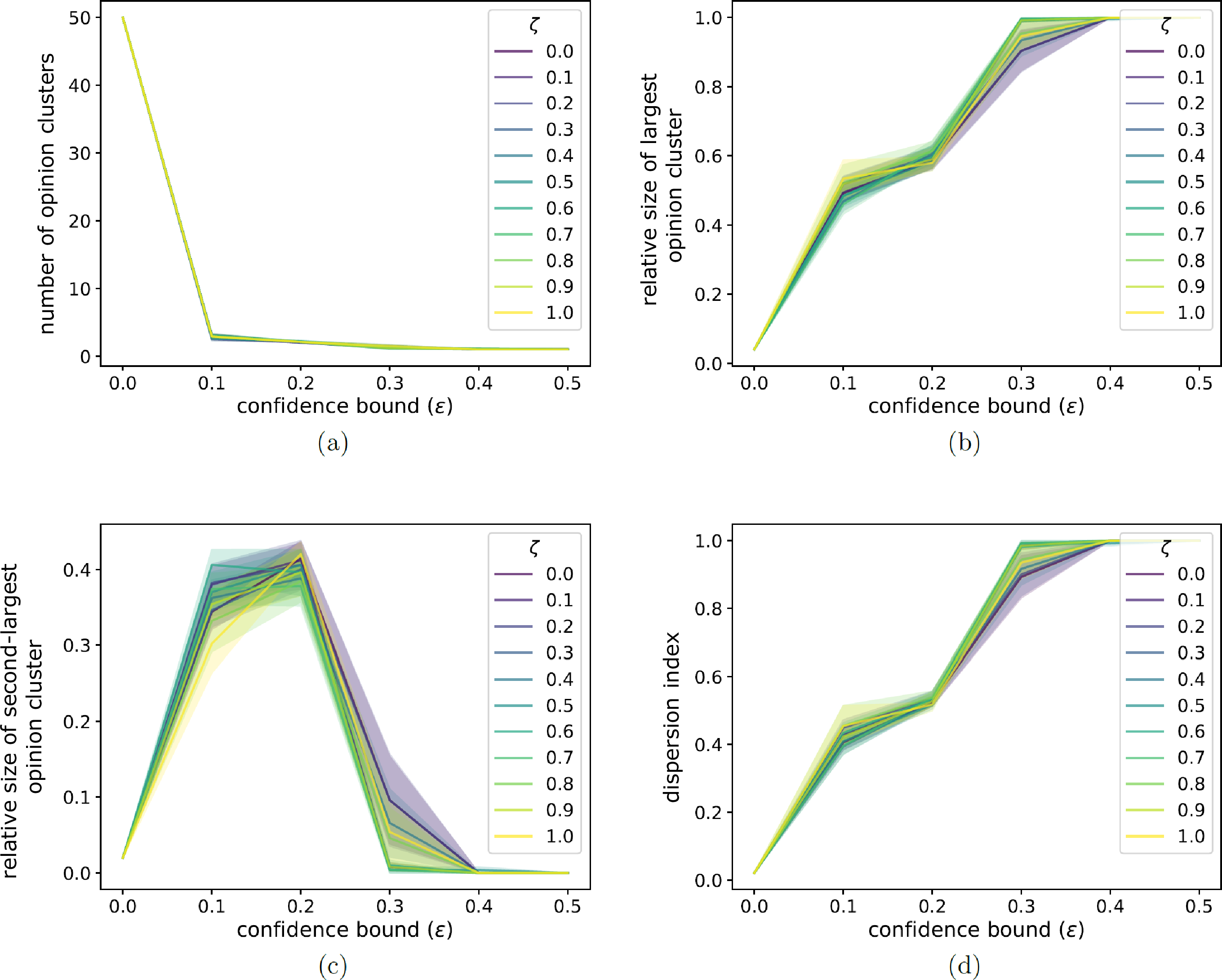
Figure 6: We illustrate the dependence of several final opinion-profile properties in our two-layer opinion–disease model on the confidence bound \(\epsilon\) for different values of the discordance threshold \(\zeta\). We show (a) the number of opinion clusters, (b) the fraction of nodes in the largest opinion cluster, (c) the fraction of nodes in the second-largest opinion cluster, and (d) the dispersion index \(d\). We initialize each network to be a \(G(N,p)\) ER graph with \(N = 50\) nodes and an independent, homogeneous probability \(p = 0.3\) of an edge between each pair of nodes. For each network, we initialize each node opinion to a uniformly random value in \([0,1]\). The neighborhood-tuning parameter is \(\sigma = 0.5\), the number of edges that we select at each discrete time for agents to interact is \(f = 0.2 N\), and the convergence parameter is \(\rho = 0.3\). The SIR model has a transmission probability of \(\beta = 0.01\) and a recovery probability of \(\gamma = 0.05\). In the disease layer, we update a network using homophilic disease-induced adaptation (see Section 6.2). Whenever a node enters compartment I, we remove \(m = 0.1 N\) of its edges; whenever a node enters compartment R, we add \(m = 0.1 N\) edges. We choose 5% of the nodes uniformly at random as initially infected; all other nodes are initially susceptible. All depicted simulations reach our stopping criterion. We plot means of 20 simulations, with the same 20 initial networks, sets of initial opinions, and sets of initially infected nodes for each curve and each panel. The shaded regions indicate the standard error.
In Fig. 6, we show the dependence of several final opinion-profile properties on the confidence bound \(\epsilon\) for different values of the discordance threshold \(\zeta\). The depicted quantities depend significantly on \(\epsilon\), but the value \(\zeta\) seems to affect them very little. We speculate that this is the case because \(\epsilon\) affects opinion updates directly, whereas \(\zeta\) only affects network rewiring.
7.3 Disease dynamics in our multilayer model↩︎
We examine the effect of the coupling between opinion and disease dynamics on the process of disease spreading. To do this, we calculate standard quantities, such as the time to steady state for the SIR dynamics, the time of peak infection, and the fraction of the population that becomes infected (and is consequently in the recovered compartment) at the end of the spreading process when no infected agents remain in the network.
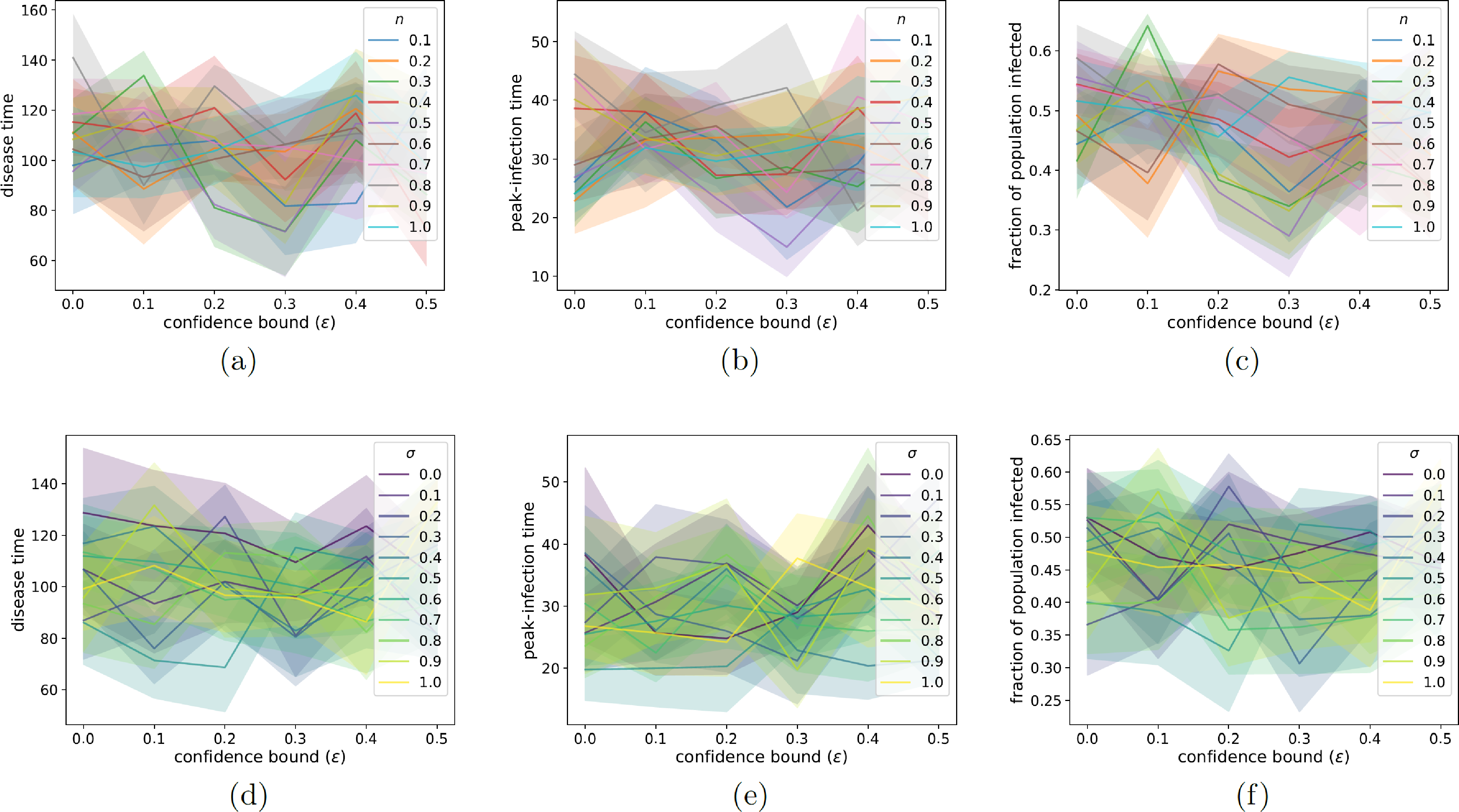
Figure 7: We examine the relationship between various properties of the disease dynamics in our two-layer opinion–disease model on the confidence bound \(\epsilon\) for (a,b,c) different values of the fraction \(n\) of edges that we choose for interactions and for (d,e,f) different values of neighborhood-tuning parameter \(\sigma\). In (a,d), we show the amount of time (the “disease time") that it takes for all infected agents to recover. In (b,e), we show the time to peak infection. In (c,f), we show the fraction of the population in the recovered state when the disease is no longer spreading. This gives the fraction of the population that becomes infected at any point. We initialize each network to be a \(G(N,p)\) ER graph with \(N = 100\) nodes and an independent, homogeneous probability \(p = 0.3\) of an edge between each pair of nodes. For each network, we initialize each node opinion to a uniformly random value in \([0,1]\). In all panels, the discordance threshold is \(\zeta = 0.2\) and the convergence parameter is \(\rho = 0.3\). The neighborhood-tuning parameter is \(\sigma = 0.5\) in panels (a,b,c) and \(n = 0.3\) in panels (d,e,f). The SIR model has a transmission probability of \(\beta = 0.01\) and a recovery probability of \(\gamma = 0.05\). In the disease layer, we update a network using homophilic disease-induced adaptation (see Section 6.2). Whenever a node enters compartment I, we remove \(m = 0.1 N\) of its edges; whenever a node enters compartment R, we add \(m = 0.1 N\) edges. We choose 5% of the nodes uniformly at random as initially infected; all other nodes are initially susceptible. We terminate a simulation either when it reaches our stopping criterion or when \(t_{\text{max}} = 2000\) time steps have elapsed (whichever occurs first). We plot means of 20 simulations, with the same 20 initial networks, sets of initial opinions, and sets of initially infected nodes for each curve and each panel. The shaded regions indicate the standard error.
In Fig. 7, we examine how the disease dynamics depends on parameters of our opinion-disease model. In Figs. 7 (a,b,c), we examine the dependence of the disease dynamics on the fraction \(n\) of edges that we choose for interactions at each discrete time. Recall that we choose \(f = nN\) edges (using \(f = \lceil nN \rceil\) if \(nN\) is not an integer) at each discrete time. In Figs. 7 (d,e,f), we examine the dependence of the disease dynamics on the neighborhood-tuning parameter \(\sigma\). The standard errors are large and it is unclear how the disease dynamics depends on \(\sigma\). This illustrates the nuanced relationship between the opinion dynamics and the disease dynamics in our two-layer opinion–disease model.
8 Conclusions and discussion↩︎
We introduced neighborhood bounded-confidence models (NBCMs) of opinion dynamics. In addition to the usual dyadic influence of BCMs, our models incorporate transitive influence in determining whether or not agents compromise their opinions when they interact with other agents. In such transitive influence, agents seek the mean opinions of the neighbors of their neighbors (e.g., friends of friends) to be sufficiently similar to their own opinions, thereby incorporating a notion of “you are who you know". We formulated neighborhood-informed generalizations of both the Hegselmann–Krause (HK) model and the Deffuant–Weisbuch (DW) model. We argued that the neighborhood HK (NHK) model includes qualitative behavior (such as changes in the order of opinions with time) that cannot occur in the standard HK model. We then illustrated the dynamics of the neighborhood DW (NDW) model using numerical computations.
We then studied our NDW model on adaptive networks, with changes in network structure that depend on neighbors of neighbors, in which agents break connections from discordant agents and then form connections to other agents. Our neighborhood-informed homophilic rewiring strategy is based on transitive homophily and yields interesting network properties. In our adaptive NDW model, we obtained a smaller degree assortativity, a smaller spectral gap, and fewer connected components than in our baseline DW model. In the adaptive NDW model, we also observed nonmonotonic behavior in the number of discordant edges as a function of time.
We then examined the interplay between opinion dynamics and disease dynamics by coupling our adaptive NDW model with an SIR compartmental model of disease spread to yield a two-layer opinion–disease model. The NDW opinion model is on one layer, the SIR model is on the other layer, and an adaptive contact network is shared by the two layers. In our opinion–disease model, the network adapts as a result of changes in both the opinion state and the disease state (i.e., both by the breaking of edges between agents with discordant opinions and by individuals becoming infected or recovering). We employed homophilic rewiring for network adaptation from both opinion dynamics and disease dynamics. In our numerical simulations of our opinion–disease model, we found that the relative contributions of dyadic opinion homophily and transitive opinion homophily had notable and unexpected effects on qualitative behavior, including the sizes of the opinion clusters. Based on our numerical computations, we observed that our model’s neighorhood-tuning parameter \(\sigma\) exerts a stronger influence on the dynamics than the discordance threshold (which determines which edges can break due to opinion differences).
Neighborhood-based transitivity — whether through transitive homophily or transitive influence — exert notable effects on human behavior [26]–[29]. It is thus important to incorporate such ideas into models of opinion dynamics. In our investigation, we have seen that our NDW model yields richer dynamics than an associated baseline DW model. We have also observed that interesting dynamics arise from incorporating transitivity into network adaptation in dynamical processes that interact through a shared adaptive network.
As with all other models of opinion dynamics, our NBCMs have several limitations. In particular, we made many simplistic assumptions about human behavior. For example, all of the agents in our models are identical and their confidence bounds are homogeneous. Naturally, it is interesting to explore heterogeneities in such features. Additionally, because our coupled opinion–disease model incorporates coupling through a common contact network, it does not account for the heterogeneous interaction structures (including both online and in-person communication and influence) in human social networks. Moreover, although our model incorporates a novel type of homophilic network adaptation, our explorations of it were minimal. It will be fascinating to systematically analyze opinion models with transitive homophily in both network adaptation and opinion dynamics.
There are a variety of ways to extend our NBCMs. These extensions include both commonly noted possibilities (such as the incorporation of multidimensional opinions, heterogeneous confidence bounds, polyadic interactions, and other models of disease spread) and generalizations that align specifically with our model’s neighborhood focus. In particular, we considered only the two-step neighbors of agents (e.g., friends of friends), and it will be interesting to examine generalizations of our NBCMs that include more expansive neighborhoods.
Code availability↩︎
Our code is available at https://bitbucket.org/neighborhood-bounded-confidence-model-of-opinion-dynamics.
Acknowledgements↩︎
MAP acknowledges financial support from the National Science Foundation (grant number 1922952) through the Algorithms for Threat Detection (ATD) program. SK acknowledges support from the UC Presidential Postdoctoral Fellowship.
References↩︎
Node \(i\)’s opinion contributes to this mean.↩︎