On open-separating dominating codes in graphs
February 05, 2024
Abstract
Using dominating sets to separate vertices of graphs is a well-studied problem in the larger domain of identification problems. In such problems, the objective is to choose a suitable dominating set \(C\) of a graph \(G\) which is also separating in the sense that the neighbourhoods of any two distinct vertices of \(G\) have distinct intersections with \(C\). Such a dominating and separating set \(C\) of a graph is often referred to as a code in the literature. Depending on the types of dominating and separating sets used, various problems arise under various names in the literature. In this paper, we introduce a new problem in the same realm of identification problems whereby the code, called open-separating dominating code, or OD-code for short, is a dominating set and uses open neighbourhoods for separating vertices. The paper studies the fundamental properties concerning the existence, hardness and minimality of OD-codes. Due to the emergence of a close and yet difficult to establish relation of the OD-code with another well-studied code in the literature called open (neighborhood)-locating dominating code (referred to as the open-separating total-dominating code and abbreviated as OTD-code in this paper), we compare the two codes on various graph families. Finally, we also provide an equivalent reformulation of the problem of finding OD-codes of a graph as a covering problem in a suitable hypergraph and discuss the polyhedra associated with OD-codes, again in relation to OTD-codes of some graph families already studied in this context.
open-separating sets ,dominating sets, total-dominating sets ,NP-completeness ,hypergraphs ,polyhedra
1 Introduction↩︎
The problem of placing surveillance devices in buildings to locate an intruder (like a fire, a thief or a saboteur) leads naturally to different separation-domination type problems in the graph modeling the building (where rooms are represented as vertices and connections between rooms as edges). Depending on the characteristics of the detection devices (to detect an intruder only if it is present in the room where the detector is installed and/or to detect one in any neighbouring room), different kinds of dominating sets can be used to detect the existence of an intruder, whereas different separation-type properties are considered to exactly locate the position of an intruder in the building.
More precisely, let \(G=(V(G), E(G)) = (V,E)\) be a graph and let \(N(v) = N_G(v) = \{u \in V : uv \in E\}\) (respectively, \(N[v] = N_G[v] = N(v) \cup \{v\}\)) denote the open neighbourhood (respectively, closed neighborhood) of a vertex \(v \in V\). A subset \(C \subseteq V\) is dominating (respectively, total-dominating) if \(N[v]\cap C\) (respectively, \(N(v)\cap C\)) is a non-empty set for each \(v \in V\). Moreover, \(C \subseteq V\) is closed-separating (respectively, open-separating) if \(N[v]\cap C\) (respectively, \(N(v)\cap C\)) is a unique set for each \(v \in V\). Furthermore, the set \(C\) is locating if \(N(v)\cap C\) is a unique set for each \(v \in V\setminus C\).
So far, the following combinations of separation and domination properties have been studied in the literature over the last decades:
closed-separation with domination and total-domination leading to identifying codes (ID-codes for short) [1] and identifying total-dominating codes1 (ITD-codes for short) [2], respectively;
location with domination and total-domination leading to locating dominating codes (LD-codes for short) [3] and locating total-dominating codes (LTD-codes for short) [2], respectively;
open-separation with total-domination leading to open-separating total-dominating codes2 (OTD-codes for short) [4], [5].
Such problems have several applications, for example, in fault-detection in multiprocessor networks [1], logical definability of graphs [6], canonical labeling of graphs for the graph isomorphism problem [7] and locating intruders in facilities using sensor networks [8], to name a few. Recall that to model the latter monitoring problems, a building is represented as a graph and the task is to place sensors at some vertices. Hereby, the subset of rooms equipped with sensors corresponds to a code in the graph, the domination properties guarantee that all rooms are monitored, whereas the separation properties ensure that the intruder can be exactly located. For monitoring systems in which each sensor can distinguish between the presence of an intruder at its own vertex and at a neighboring vertex, the separating property useful in pinpointing the intruder is location [3]. On the other hand, if some sensors lose the ability to distinguish between the presence of an intruder at their own vertex and a neighboring one, then the separating property required to locate the intruder is that of closed-separation [1]. Finally, if some sensor in the monitoring system is disabled by an intruder, then the separating property useful in locating the intruder is that of open-separation [4], [5]. For more applications and results, we refer to an extensive internet bibliography containing over 500 articles around these topics maintained by Jean and Lobstein [9].
In this paper, we aim at studying open-separation combined with domination. We call a subset \(C \subseteq V\) of a graph \(G=(V,E)\) an open-separating dominating code (OD-code for short) if it is
a dominating set, that is \(N[v]\cap C\) is a non-empty set for each \(v \in V\); and
an open-separating set, that is \(N(v)\cap C\) is a unique set for each \(v \in V\).
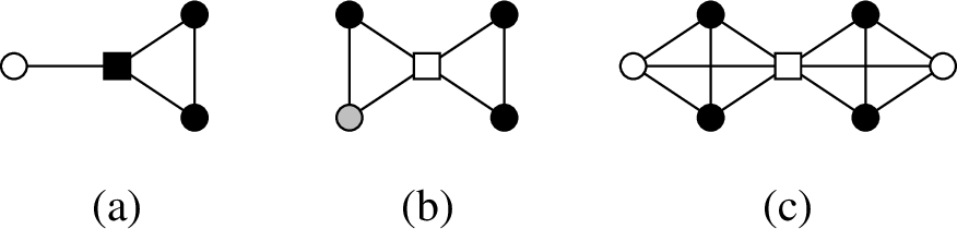
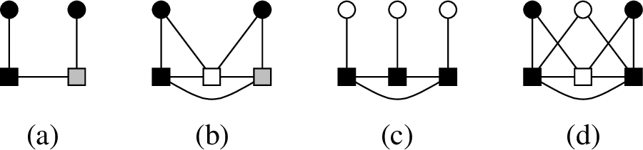
As is evident from the definitions, the OD-code is a variation of the OTD-code which combines open-separation with total-domination. In the literature of domination-based identification problems, the OTD-code has been quite well studied, for example, in [5], [10]–[23]. The OD-code, however, has so far not been studied in the literature of identification problems except for in the conference proceeding [24] of the current paper where some of the same results have appeared without proofs. The motivation to combine open-separation with domination to study the OD-codes is a most natural one, as has been the case with other separation properties like location and closed-separation which have also been studied in combination with both domination and total-domination. Figure 1 illustrates examples of such codes in a small graph.

Note that not all graphs admit codes of all the studied types. Accordingly, in Section 2 of this paper, we address the conditions for the existence of OD-codes and their relations to codes of other types. It turns out that OD-codes possess a particularly close relationship with OTD-codes as the minimum cardinalities of the two differ by at most one. Moreover, for any \({\mathrm{\small X}}\in \{{\mathrm{\small ID}}, {\mathrm{\small ITD}}, {\mathrm{\small LD}}, {\mathrm{\small LTD}}, {\mathrm{\small OTD}}\}\), the problem of determining an X-code of minimum cardinality \(\gamma^{X}(G)\) of a graph \(G\), called the X-number of \(G\), has been shown to be NP-hard [5], [25], [26]. In Section 3, we show that NP-hardness holds for OD-codes as well. This also enables us to reprove the NP-hardness of the OTD-problem on a narrower class of input graphs and with an arguably simpler reduction than previously considered, for example, in [5], [22]. Furthermore, despite the close relationship between the OD- and OTD-numbers of a graph, we show that deciding whether the two numbers differ is NP-hard. This motivates us to compare the OD- and the OTD-codes of graphs of different families in Section 4 and to study their related polyhedra in Section 5. We close with some concluding remarks and lines of future research.
Further terminologies and notations↩︎
A graph \(H\) is called a subgraph of a graph \(G\) if \(V(H) \subseteq V(G)\) and \(E(H) \subseteq E(G)\). Moreover, a subgraph \(H\) of \(G\) is said to be induced if \(uv \in E(H)\) if and only if \(uv \in E(G)\). For an induced subgraph \(H\) of \(G\), if \(S = V(H)\), then \(H\) is said to be induced by \(S\) and is denoted \(G[S]\). The girth of a given graph \(G\) is the smallest length of an induced cycle in \(G\). The degree of a vertex \(v\), denoted \(\deg(v) = \deg_G(v)\), is the number of neighbors of \(v\) in \(G\). A vertex of degree \(0\) is called an isolated vertex, a vertex of degree \(1\) is called a leaf and the neighbor of a leaf is called the support vertex of the leaf. Given any two vertices of \(u,v\) of a graph \(G\), the distance between them, denoted \(d(u,v) = d_G(u,v)\), is the length of the shortest induced path in \(G\) with \(u\) and \(v\) as its endpoints. A graph is said to be complete (on \(n\) vertices), and denoted \(K_n\), if any two of its vertices are adjacent. A clique is a vertex subset \(S\) of a graph \(G\) such that the subgraph of \(G\) induced by \(S\) is complete. On the other hand, a stable set is a vertex subset \(S\) of a graph \(G\) such that no two vertices in \(S\) are adjacent in \(G\). A graph \(G=(U \cup W, E)\) is bipartite if its vertex set can be partitioned into two stable sets \(U\) and \(W\) so that every edge of \(G\) has one endpoint in \(U\) and the other in \(W\). A graph \(G=(Q \cup S, E)\) is a split graph if its vertex set can be partitioned into a clique \(Q\) and a stable set \(S\). Given two graphs \(G_1\) and \(G_2\) whose vertex sets are disjoint, the graph \((V(G_1) \cup V(G_2), E(G_1) \cup E(G_2))\) is denoted by \(G_1 \oplus G_2\).
A vertex \(w \in V\) is said to open-separate two distinct vertices \(u,v \in V\) if \(w \in N(u) \bigtriangleup N(v)\). Moreover, a vertex subset \(S\) of \(G\) is said to open-separate the pair \(u,v\) (by a vertex \(w\)) if \(w \in S\) such that \(w\) open-separates \(u,v\). Then, it can be verified that a set \(S\) has the open-separating property (defined before) if and only if it open-separates every pair of distinct vertices of \(G\).
2 Reformulation, existence and bounds↩︎
In this section, we reformulate the OD-problem, address fundamental questions concerning the existence of OD-codes and bounds for OD-numbers.
2.1 Hypergraph representation of the OD-problem↩︎
Given a graph \(G=(V,E)\) and a problem X, we look for a hypergraph \(\mathcal{H}_{\mathrm{\small X}}(G) = (V,\mathcal{F}_{\mathrm{\small X}})\) so that \(C \subset V\) is an X-code of \(G\) if and only if \(C\) is a cover of \(\mathcal{H}_{\mathrm{\small X}}(G)\) satisfying \(C \cap F \neq \emptyset\) for all \(F \in \mathcal{F}_{\mathrm{\small X}}\). Then the covering number \(\tau(\mathcal{H}_{\mathrm{\small X}}(G))\), defined as the minimum cardinality of a cover of \(\mathcal{H}_{\mathrm{\small X}}(G)\), equals by construction the X-number \(\gamma^{\rm{X}}(G)\) of \(G\). The hypergraph \(\mathcal{H}_{\mathrm{\small X}}(G)\) is called the X-hypergraph of the graph \(G\).
It is a simple observation that for an X-problem involving domination (respectively, total-domination), \(\mathcal{F}_{\mathrm{\small X}}\) needs to contain the closed (respectively, open) neighborhoods of all vertices of \(G\). In order to encode the separation of vertices, that is, the fact that the intersections of an X-code \(C\) with the neighborhood of each vertex is unique, it was suggested in [11], [27] to use the symmetric differences of the neighborhoods. Here, given two sets \(A\) and \(B\), their symmetric difference is defined by \(A \Delta B = (A \setminus B) \cup (B \setminus A)\). In fact, it has been shown in [11], [27] that a code \(C\) of a graph \(G\) is closed-separating (respectively, open-separating) if and only if \((N[u] \Delta N[v]) \cap C \neq \emptyset\) (respectively, \((N(u) \Delta N(v)) \cap C \neq \emptyset\)) for all pairs of distinct vertices \(u,v\) of \(G\). This implies for OD-codes:
Corollary 1. The OD-hypergraph \(\mathcal{H}_{{\mathrm{\small OD}}}(G) = (V,\mathcal{F}_{{\mathrm{\small OD}}})\) of a graph \(G=(V,E)\) is composed of
the closed neighborhoods \(N[v]\) of all vertices \(v \in V\) and
the symmetric differences \(N(u) \Delta N(v)\) of open neighborhoods of distinct vertices \(u,v \in V\)
as hyperedges in \(\mathcal{F}_{{\mathrm{\small OD}}}\) and \(\gamma^{\rm{OD}}(G)=\tau(\mathcal{H}_{{\mathrm{\small OD}}}(G))\) holds.
2.2 Existence of OD-codes↩︎
It has been observed in the literature that the studied domination and separation properties may not apply to all graphs, see for example [1], [2], [5]. More precisely,
total-domination excludes the occurrence of isolated vertices in graphs, that is, vertices \(v\) with \(N(v) = \emptyset\);
closed-separation (respectively, open-separation) excludes the occurrence of closed twins (respectively, open twins), that is, distinct vertices \(u,v\) with \(N[u] = N[v]\) (respectively, \(N(u) = N(v)\)).
Calling a graph \(G\) to be X-admissible if \(G\) has an X-code, we see that while, for example, every graph \(G\) is LD-admissible, a graph \(G\) is OTD-admissible if and only if \(G\) has neither isolated vertices nor open twins. Accordingly, we conclude the following regarding the existence of OD-codes of graphs.
Corollary 2. A graph \(G\) is OD-admissible if and only if \(G\) has no open twins.
Since any two distinct isolated vertices of a graph are open twins with the empty set as both their open neighbourhoods, Corollary 2 further implies that an OD-admissible graph has at most one isolated vertex.
2.3 Bounds on OD-numbers and their relations to other X-numbers.↩︎
Remark 1. Let \(G\) be an OD-admissible graph and let \(C\) be an OD-code of \(G\). Then, there exists at most one vertex \(w\) of \(G\) such that \(N(w) \cap C=\emptyset\).
Proof. Toward contradiction, if there exist two distinct vertices \(u\) and \(v\) of \(G\) such that \(N(u) \cap C = N(v) \cap C = \emptyset\), then \(C\) does not open-separate the pair \(u,v\), a contradiction. This proves the result. ◻
Remark 2. Let \(G\) be an OD-admissible graph and let \(C\) be a dominating set of \(G\) such that there exists at most one vertex \(w\) of \(G\) with \(N(w) \cap C=\emptyset\). If the set \(C\) open-separates every pair \(u,v\) of distinct vertices of \(G\) with \(d(u,v) \leq 2\), then \(C\) is an OD-code of \(G\).
Proof. It is enough to show that \(C\) open-separates every pair \(u,v\) of distinct vertices of \(G\) such that \(d(u,v) \geq 3\). So, assume that \(u\) and \(v\) are two such vertices of \(G\) with \(d(u,v) \geq 3\). Then, we have \(N(u) \triangle N(v) = N(u) \cup N(v)\). If \(C\) does not open-separate the pair \(u,v\), then it implies that \(C\) does not intersect \(N(u) \cup N(v)\), that is, \(N(u) \cap C = N(v) \cap C = \emptyset\), which contradicts our assumption. Therefore, \(C\) open-separates \(u,v\) and this proves the result. ◻
We now prove general upper and lower bounds on the OD-number of a graph in terms of its order, that is the number of vertices. The proof for these bounds involves the following result due to Bondy.
Theorem 1 (Bondy [28]). Let \(C\) be a set with \(|C| = n\) and let \(C_1, C_2, \ldots , C_n\) be subsets of \(C\) for each \(i \in [n]\) such that \(C_i \neq C_j\) for each \(i,j \in [n]\) and \(i \neq j\). Then, there exists an element \(x\) of \(S\) such that \(C_i \setminus \{x\} \neq C_j \setminus \{x\}\) for each \(i,j \in [n]\) and \(i \neq j\).
Lemma 1. Let \(G_1\) and \(G_2\) be OD-admissible graphs on disjoint vertex sets each of whose cardinalities is at least two. Let \(G = G_1 \oplus G_2\) be their disjoint union. If \(S_1\) is an OD-code of \(G_1\), then the set \(S = S_1 \cup V(G_2)\) is an OD-code of \(G\).
Proof. Clearly, the set \(S\) is a dominating set of \(G\) since \(S_1\) is a dominating set of \(G_1\). Let \(u,v\) be two distinct vertices of \(G\). Then, we show that the set \(S\) has non-empty intersection with \(N_G(u) \bigtriangleup N_G(v)\). If \(u,v \in V(G_1)\), then we have \(N_G(u) \bigtriangleup N_G(v) = N_{G_1}(u) \bigtriangleup N_{G_1}(v)\). Since \((N_{G_1}(u) \bigtriangleup N_{G_1}(v)) \cap S_1 \ne \emptyset\) due to \(S_1\) being an OD-code of \(G_1\), we have \((N_G(u) \bigtriangleup N_G(v)) \cap S \ne \emptyset\). Now if \(u,v \in V(G_2)\), then \(N_G(u) \bigtriangleup N_G(v) = N_{G_2}(u) \bigtriangleup N_{G_2}(v) \ne \emptyset\) since \(G_2\) is X-admissible. This implies that \((N_{G_2}(u) \bigtriangleup N_{G_2}(v)) \cap V(G_2) \ne \emptyset\) and hence, \((N_G(u) \bigtriangleup N_G(v)) \cap S \ne \emptyset\). Finally, let us assume that \(u \in V(G_1)\) and \(v \in V(G_2)\). Since \(G_2\) is on at least two vertices, this implies that there exists a vertex \(v' \in N_{G_2}(v) \subseteq S\) with \(v' \ne v\). Now, since \(N_G(u) \bigtriangleup N_G(v) = N_{G_1}(u) \cup N_{G_2}(v)\), we have \(v' \in (N_G(u) \cup N_G(v)) \cap S\). This proves the result. ◻
Theorem 2. For a graph \(G\) on \(n \geq 2\) vertices without open twins and any isolated vertices, we have \(\lceil \log n \rceil \leq \gamma^{\rm{OD}}(G) \leq n-1\).
Proof. Let us first prove the result on the lower bound of \(\gamma^{\rm{OD}}(G)\). Let \(S\) be a minimum OD-code of \(G\), that is, \(|S| = \gamma^{\rm{OD}}(G)\). Then, for each vertex \(v \in V(G)\), the subset \(N(v) \cap S \subset S\) is unique. In other words, the number \(n\) of vertices of \(G\) can be at most the number of subsets of \(S\) which is \(2^{|S|}\). This implies that \(\log n \le |S| = \gamma^{\rm{OD}}(G)\) which further implies \(\lceil \log n \rceil \le \gamma^{\rm{OD}}(G)\), since the OD-number is an integer.
We now prove the result on the upper bound of \(\gamma^{\rm{OD}}(G)\). Since \(G\) is without isolated vertices, it must have at least one edge. So, let \(G_1\) be a component of \(G\) with at least one edge and of order \(n_1\). Then, \(G_1\) is also OD-admissible. Let \(G_2\) be the disjoint union of all components of \(G\) other than \(G_1\). In other words, we have \(G = G_1 \oplus G_2\). Let \(S_1\) be a minimum OD-code of \(G_1\), that is, \(|S_1| = \gamma^{\rm{OD}}(G_1)\). Now, if \(\gamma^{\rm{OD}}(G_1) \le n_1-1\), then, by applying Lemma 1, the set \(S = S_1 \cup V(G_2)\) is an OD-code of \(G\). This implies that \(\gamma^{\rm{OD}}(G_1) \le |S| \le n-1\).
Therefore, let us assume that \(\gamma^{\rm{OD}}(G_1) = |S_1| = n_1\), that is, \(S_1 = V(G_1)\). Now, let \(V(G_1)=\{v_1, v_2, \ldots v_{n_1}\}\) and let \(C_i = N(v_i)\) for each \(i \in [n_1]\). Since \(S_1\) is an OD-code of \(G_1\), we have \(C_i \neq C_j\) for all \(i, j \in [n_1]\) and \(i \neq j\). However, by Theorem 1 (Bondy’s theorem), there exists a vertex \(x_1\) of \(G_1\) such that \(C_i \setminus \{x_1\} \neq C_j \setminus \{x_1\}\) for all \(i, j \in [n_1]\) and \(i \neq j\). In other words, the set \(S_1 \setminus \{x_1\}\) is an open-separating set of \(G_1\). Moreover, \(S_1\setminus \{x_1\}\) is also a dominating set of \(G_1\), since \(S_1 \setminus \{x_1\} = V(G_1) \setminus \{x_1\}\) and \(G_1\) is connected. Thus, \(S_1 \setminus \{x_1\}\) is an OD-code of \(G_1\) which is a contradiction to the minimality of \(S_1\) in being an OD-code of \(G_1\). Therefore, we have \(\gamma^{\rm{OD}}(G_1) \leq n_1-1\) and we are again done by Lemma 1. ◻
Both bounds in Theorem 2 are tight. For the lower bound, an example of a graph whose OD-number attains the bound would be a split graph, say \(G=(K \cup S, E)\), where \(K \cong K_{2n+1}\) and \(S\) is a stable set such that for all subset \(U\) of \(V(K)\) with \(|U| \notin \{0,2n\}\), there exists a vertex \(v \in S\) with \(N(v) = U\). Examples of graphs whose OD-number attains the upper bound in Theorem 2 are addressed in Section 4.
Next, we turn to the relation of OD-numbers to other X-numbers for \({\mathrm{\small X}}\in \{{\mathrm{\small LD}}, {\mathrm{\small LTD}}, {\mathrm{\small ID}}, {\mathrm{\small ITD}}, {\mathrm{\small OTD}}\}\). The next theorem brings out a close association between the OD- and the OTD-numbers of an OTD-admissible graph.
Theorem 3. Let \(G\) be an OD-admissible graph.
If \(G\) is a disjoint union of a graph \(G'\) and an isolated vertex, then we have \(\gamma^{\rm{OD}}(G) = \gamma^{\rm{OTD}}(G') + 1\).
If \(G\) is OTD-admissible, we have \(\gamma^{\rm{OTD}}(G) - 1 \leq \gamma^{\rm{OD}}(G) \leq \gamma^{\rm{OTD}}(G)\).
Proof. Let us first assume that \(G = G' \oplus \{v\}\) for some vertex \(v\) of \(G\). Moreover, let \(C\) be any minimum OD-code of \(G\). Then, \(v \in C\) in order for \(C\) to dominate \(v\). This implies that \(N(v) \cap C = \emptyset\). Therefore, by Remark 1, the set \(C \setminus \{v\}\) must total-dominate all vertices in \(V \setminus \{v\}\), that is, \(C\) is an OD-code of \(G'\). This implies that \(\gamma^{\rm{OTD}}(G') \leq |C| - 1 = \gamma^{\rm{OD}}(G)-1\), that is, \(\gamma^{\rm{OD}}(G) \leq \gamma^{\rm{OTD}}(G') + 1\). On the other hand, if \(C'\) is an OTD-code of \(G'\), then \(C' \cup \{v\}\) is an OD-code of \(G\). This implies that \(\gamma^{\rm{OD}}(G) \leq |C'|+1 = \gamma^{\rm{OTD}}(G')+1\) and hence, assertion (a) follows.
Let us now assume that \(G\) has no isolated vertices. Then, \(G\) is also OTD-admissible. Now, the inequality \(\gamma^{\rm{OD}}(G) \leq \gamma^{\rm{OTD}}(G)\) holds by the fact that any OTD-code of \(G\) is also a dominating and an open-separating set of \(G\) and hence, is an OD-code of \(G\). To prove the other inequality, we let \(C\) be a minimum OD-code of \(G\). Then, we have \(|C| = \gamma^{\rm{OD}}(G)\). Now, if \(C\) is also an OTD-code of \(G\), then the result holds trivially. Therefore, let us assume that \(C\) is not an OTD-code of \(G\), that is, in particular, \(C\) is not a total-dominating set of \(G\). This implies that there exists a vertex \(v\) of \(G\) such that \(C \cap N(v) = \emptyset\). Moreover, by Remark 1, \(C \cap N(v)=\emptyset\) for exactly the vertex \(v\) of \(G\). This implies that \(C \cup \{v\}\) is a total-dominating set of \(G\) and hence, is also an OTD-code of \(G\). Therefore, we have \(\gamma^{\rm{OTD}}(G) \leq |C|+1 = \gamma^{\rm{OD}}(G) +1\) which implies assertion (b). ◻
We next address the relation of OD-numbers to LD- and LTD-numbers of a graph.
Theorem 4. Let \(G\) be an OD-admissible graph.
We have \(\gamma^{\rm{LD}}(G) \le \gamma^{\rm{OD}}(G)\).
If \(G\) has no isolated vertex, then we have \(\gamma^{\rm{LTD}}(G) - 1 \leq \gamma^{\rm{OD}}(G)\).
Proof. We clearly have, by definition, that every open-separating set of a graph \(G\) is also a locating set of \(G\). Hence, every OD-code of \(G\) is also an LD-code of \(G\) and assertion (a) follows. Moreover, if \(G\) has no isolated vertex, then every OTD-code of \(G\) is also an LTD-code of \(G\) which implies that \(\gamma^{\rm{LTD}}(G) \leq \gamma^{\rm{OTD}}(G)\) holds. Combining the latter inequality with Theorem 3(b), we further conclude \[\gamma^{\rm{LTD}}(G) - 1 \leq \gamma^{\rm{OTD}}(G)- 1 \leq \gamma^{\rm{OD}}(G)\] which implies assertion (b). ◻
On the other hand, there exist graphs \(G\) with \(\gamma^{\rm{OD}}(G) < \gamma^{\rm{LTD}}(G)\) and the OD-numbers of graphs are not generally comparable to their ID- and ITD-numbers, see Table 2 for an illustration.

3 Computational complexity of the OD-problem↩︎
It has been established in the literature that all the previously studied X-problems are NP-hard [5], [25], [26]. We next address the computational complexity of the decision version of the OD-problemdefined as follows.
In this section, we shall prove that -Code is NP-complete. Apart from that, we also consider in this section the computational complexity of another related problem as we now describe. By Theorem 3(b), given an OTD-admissible graph \(G\), we have either \[\gamma^{\rm{OTD}}(G) = \gamma^{\rm{OD}}(G)~~ \text{ or }~~ \gamma^{\rm{OTD}}(G) = \gamma^{\rm{OD}}(G)+1.\] However, despite this small difference (of at most \(1\)) between the two code-numbers, we show that it is NP-hard to decide in general if they are equal or different on any given OTD-admissible graph. This is equivalent to simply proving that it is NP-hard to decide if \(\gamma^{\rm{OTD}}(G) = \gamma^{\rm{OD}}(G) + 1\). We now define the decision version of this problem as the following.
As can be noticed in OTD= OD+1, given a vertex subset \(S\) (with \(|S| = k\)) of an input graph \(G\) on \(n\) vertices, to check condition (c), one has to consider all subsets of \(V(G)\) of order \(k-1\) (which admits a running time of \(\mathcal{O}(n^{k-1})\)) and check if \(S\) is an OTD-code (which admits a running time of \(\mathcal{O}(n^2)\)). In other words, verifying a certificate for OTD= OD+1 can potentially take up to a running time of order \(\mathcal{O}(n^{k-1}) \cdot \mathcal{O}(n^2) \subseteq \mathcal{O}(n^{k+1})\). Since we have \(k = |S| \in \mathcal{O}(n)\), it implies that verifying a certificate for this problem may not necessarily be a polynomial-time algorithm. This implies that, OTD= OD+1 does not necessarily belong to the class NP. Nevertheless, we show that the problem is still NP-hard.
To prove the hardness of the above two decision problems, we use Linear SAT, or LSAT — a variation of 3-SAT — which is defined as follows.
LSAT was proven to be NP-complete by Arkin et al. in [29]. From here on, we shall denote by \(\psi = (X, \mathcal{C})\) a generic instance defined on the set of Boolean variables \(X\) and the set of clauses \(\mathcal{C}\). In addition, let \(n = |X|\) and \(m = |\mathcal{C}|\) and let us denote by \(\phi = \phi(\mathcal{C})\) the Boolean formula defined by \(\phi = \mathbf{c_1} \wedge \mathbf{c_2} \wedge \ldots \wedge \mathbf{c_m}\), where \(\mathbf{c_i} \in \mathcal{C}\) for all \(1 \le i \le m\). We may also assume from here on that no clause contains both literals of a variable, as such a clause is always satisfiable.
We now introduce the following variation of LSAT where we require that if a literal from \(X\) appears in a clause, it must appear in exactly two clauses.
Let the auxiliary graph of SL-SAT be the bipartite graph where one part of the vertex set is \(\mathcal{C}\) and the other the set of all literals from \(X\). Moreover, let the edge set of the auxiliary graph consist of edges \(x \mathbf{c}\), where \(x\) is a literal from \(X\) belonging to the clause \(\mathbf{c} \in \mathcal{C}\).
Remark 3. The auxiliary graph of SL-SAT is bipartite, of maximum degree \(3\) and is of girth at least \(6\).
Proof. Let \(H\) be the auxiliary graph of SL-SAT. Then \(H\) is bipartite by construction.
Each vertex of \(H\) corresponding to the literals from \(X\) has degree \(2\) (since a literal belongs to at most two clauses); and each vertex of \(H\) corresponding to the clauses in \(\mathcal{C}\) has degree at most \(3\) (since each clause contains at most \(3\) literals). This proves the result on the maximum degree of \(H\).
Finally, \(H\) cannot contain an induced four-cycle as it would imply that there exist two clauses having two literals in common which contradicts the input constraint of SL-SAT. Moreover, since \(H\) is bipartite and hence, contains only even cycles, all induced cycles in \(H\) must be of length at least \(6\). This proves the result on the girth of \(H\). ◻
We shall next prove that SL-SAT is NP-complete using the following reduction from an instance \(\psi = (X,\mathcal{C})\) of LSAT to an instance \(\psi' = (X', \mathcal{C}')\) of SL-SAT.
Reduction 1. Let \(\phi\) be the Boolean formula of LSAT with respect to \(X\) and \(\mathcal{C}\). Then the reduction starts with \(X' = X\), \(\mathcal{C}' = \mathcal{C}\) and \(\phi' = \phi\). It then runs over all literals from \(X\). At each step, if a literal, say \(x\), appears in only one clause of \(\phi\), the reduction creates an auxiliary variable \(y\) and updates the set of variables \(X' \leftarrow X' \cup \{y\}\), the set of clauses \(\mathcal{C}' \leftarrow \mathcal{C}' \cup \{(x \vee y), (y)\}\) and also appends the formula \(\phi \leftarrow (x \vee y) \wedge (y) \wedge \phi\). At the end of the reduction, the resulting \(\psi' = (X', \mathcal{C}')\) is an instance of SL-SAT.
It can be verified that, at the end of Reduction 1, we have \(|X'| \le 3n\) and \(|\mathcal{C}| \le m + 4n\). Moreover, the reduction is clearly polynomial-time in \(n+m\).
Lemma 2. SL-SAT is NP-complete.
Proof. Clearly, SL-SAT belongs to the class NP. Let \(X' = X \cup Y\) and \(\phi' = \phi \wedge \mu\), where \(Y\) is the set of auxiliary variables introduced in Reduction 1 and \(\mu\) is the Boolean formula obtained by appending the clauses in Reduction 1. Note that \(\phi\) has literals only from \(X\).
To prove the necessary part of the NP-hardness, let \(\psi = (X, \mathcal{C})\) be a Yes-instance of LSAT and so, let \(A : X \to \{0,1\}\) be a satisfying assignment on \(X\). Then, we create an assignment \(A' : X' \to \{0,1\}\) by requiring \(A'(x) = A(x)\) if \(x \in X\) and \(A'(x) = 1\) if \(x \in Y\). Then it is clear that this is a satisfying assignment on \(X'\) since \(\phi' = \phi \wedge \mu\) and each clause in \(\mu\) has an auxiliay variable which is assigned to \(1\) by \(A'\). Hence, \(\psi' = (X', \mathcal{C}')\) is a Yes-instance of SL-SAT.
To prove the sufficiency part of the NP-hardness, if \(\psi'\) is a Yes-instance of SL-SAT and \(A' : X' \to \{0,1\}\) is a satisfying assignment on \(X'\), we create an assignment of \(A : X \to \{0,1\}\) by requiring \(A(x) = A'(x)\). Again, \(\phi' = \phi \wedge \mu\) implies that \(A\) is a satisfying assignment on \(X\). Hence, \(\psi\) is a Yes-instance of LSAT. ◻
We now come to the main results of this section and their proofs. To that end, we describe the following reduction from SL-SAT to both -Code and OTD= OD+1.
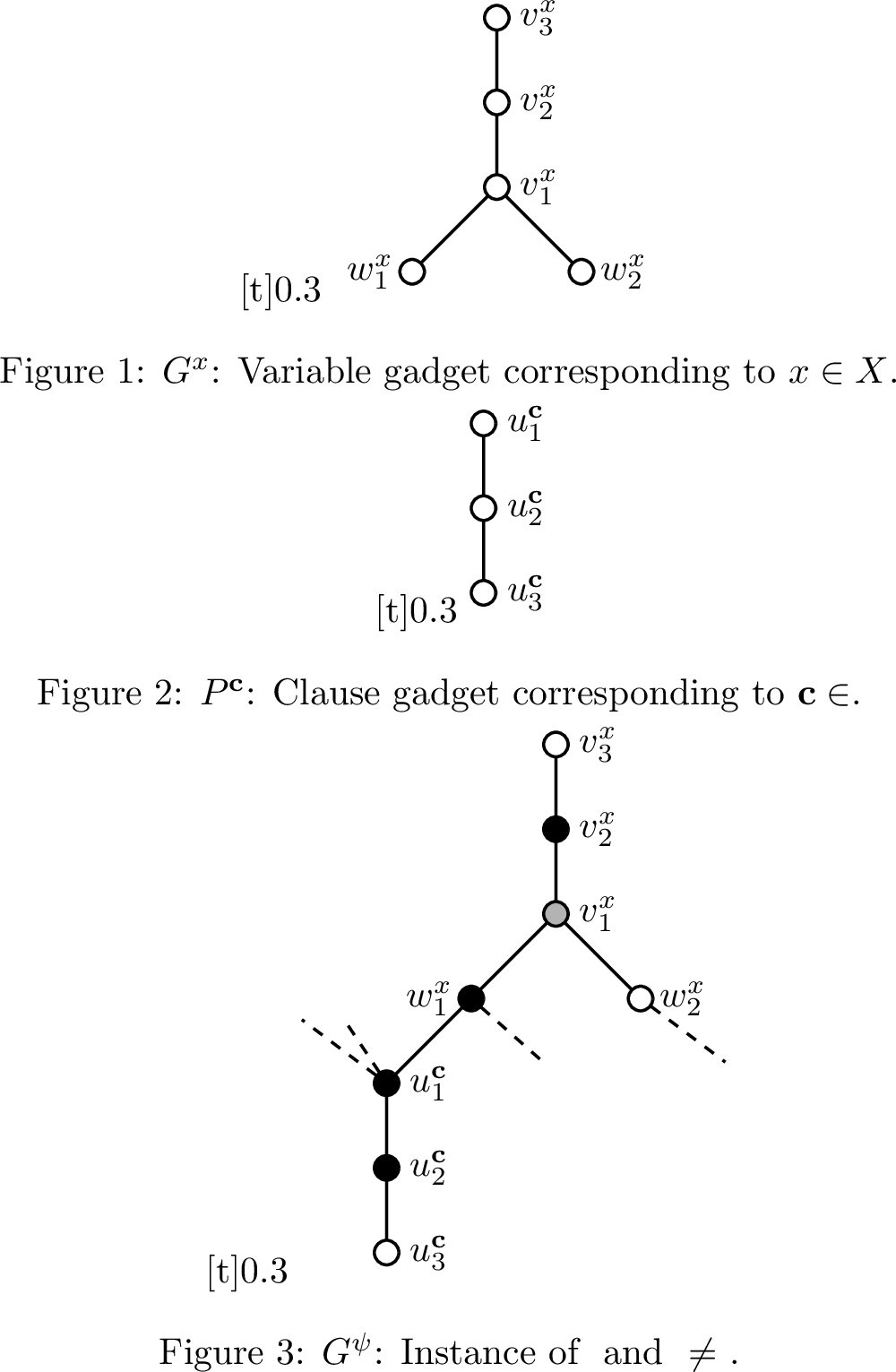
Reduction 2. The reduction takes as input an instance \(\psi = (X,\mathcal{C})\) of SL-SAT. Also, let \(\phi\) be the Boolean formula of SL-SAT. The reduction constructs a graph \(G^\psi\) as follows (also refer to Figure 3):
For every variable \(x \in X\), do the following (refer to Figure [fig95NP32Variable95OD]):
Add a vertex named \(w^x_1\) if the literal \(x\) appears in the formula \(\phi\); and add a vertex named \(w^x_2\) if the literal \(\neg x\) appears in the formula \(\phi\). For the rest of the reduction, we assume that both \(w^x_1\) and \(w^x_2\) exist; and in case one of them does not, the corresponding action related to the vertex described in this reduction does not take place.
Add 3 vertices named \(v^x_1\), \(v^x_2\) and \(v^x_3\) and add edges \(v^x_1 w^x_1\), \(v^x_1 w^x_2\) and the edges \(v^x_1 v^x_2\) and \(v^x_2 v^x_3\) (the last two edges make the vertices \(v^x_1\), \(v^x_2\) and \(v^x_3\) induce a \(P_3\)).
Let the graph induced by the above 5 (or 4) vertices be denoted as \(G^x\) and be called the variable gadget* corresponding to the variable \(x \in X\).*
For every clause \(\mathbf{c} \in \mathcal{C}\), do the following (refer to Figure [fig95NP32Clause95OD]):
- Add 3 vertices named \(u^x_1\), \(u^x_2\) and \(u^x_3\) and add edges \(u^x_1u^x_2\) and \(u^x_2u^x_3\) thus making \(u^x_1\), \(u^x_2\) and \(u^x_3\) induce a \(P_3\).
Let the \(P_3\) induced by the above 3 vertices be denoted by \(P^\mathbf{c}\) and be called the clause gadget* corresponding to the clause \(\mathbf{c} \in \mathcal{C}\).*
For all variables \(x \in X\) and all clauses \(\mathbf{c} \in \mathcal{C}\), if the literal \(x\) is in a clause \(\mathbf{c}\), then add the edge \(u^\mathbf{c}_1w^x_1\); and if the literal \(\neg x\) is in a clause \(\mathbf{c}\), then add the edge \(u^\mathbf{c}_1w^x_2\) (refer to Figure [fig95NP32G95I95OD]).
As a matter of notation, for any variable \(x \in X\), let us denote by \([x]\) the set \(\{x,\neg x\}\). Moreover, in all the proofs that follow in this section, we also assume that both the vertices \(w^x_1\) and \(w^x_2\), for \(x \in X\), exist in the graph \(G^\psi\). In case one of them does not and the analysis changes as a result of that, we shall point that out accordingly.
Lemma 3. For an instance \(\psi = (X,\mathcal{C})\) of SL-SAT with \(|X|=n\) and \(|\mathcal{C}|=m\), let \(G^\psi\) be as in Reduction 2. Moreover, let \(T = \{(v^x_1, v^x_2, v^x_3) : x \in X\} \cup \{(u^\mathbf{c}_1,u^\mathbf{c}_2, u^\mathbf{c}_3) : \mathbf{c} \in \mathcal{C}\}\). Then, for an open-separating set \(S\) of \(G^\psi\), the following assertions are true.
If \(S\) is an OTD-code of \(G^\psi\), then \(|T \cap S| \ge 2n+2m\).
If \(S\) is an OD-code of \(G^\psi\), then \(|T \cap S| \geq 2n+2m-1\).
Moreover, we have \(\gamma^{\rm{OTD}}(G^\psi) \geq 3n+2m\) and \(\gamma^{\rm{OD}}(G^\psi) \geq 3n+2m-1\).
Proof. (1) Let \(S\) be an OTD-code of \(G^\psi\). Then, for each \((v_1,v_2,v_3) \in T\), the vertex \(v_2\) must belong to \(S\) for the latter to total-dominate \(v_3\). Moreover, at least one vertex from the pair \((v_1,v_3)\) must be in \(S\) for the latter to total-dominate the vertex \(v_2\). In total therefore, counting over all the \(n\) variable gadgets and \(m\) clause gadgets, we have \(|T \cap S| \geq 2n+2m\).
(2) Let \(S\) be an OD-code of \(G^\psi\). Now, if at least two vertices out of each triple \((t_1,t_2,t_3) \in T\) belong to \(S\), then we have \(|S| \geq 2n+2m > 2n+2m-1\) and thus, we are done. So, let us assume that there exists one triple \((t^\star_1,t^\star_2,t^\star_3) \in T\) which has at most one vertex in \(S\). However, every triple \((t_1,t_2,t_3) \in T\) must have at least one of \(t_2\) and \(t_3\) in \(S\) in order for the latter to dominate \(t_3\). This implies that exactly one of \(t^\star_2\) and \(t^\star_3\) belongs to \(S\). This further implies that either \(N_{G^\psi}(t^\star_2) \cap S = \emptyset\) or \(N_{G^\psi}(t^\star_3) \cap S = \emptyset\). This further implies that each triple of \(T\) other than \((t^\star_1,t^\star_2,t^\star_3)\) has at least two vertices in \(S\) (or else, two vertices of \(G^\psi\) would have empty neighborhoods in \(S\) and hence, the pair would not be open-separated by \(S\), a contradiction). Thus, again counting over all the \(n\) variable gadgets and \(m\) clause gadgets, we have \(|S| \geq 2n+2m-1\).
Finally, in each of the above two cases, since \(S\) is an open-separating set of \(G^\psi\), at least one of \(w^x_1\) and \(w^x_2\) must be in \(S\) in order for the latter to open-separate the pair \(v^x_1, v^x_3\). This implies the final statement of the result. ◻
Lemma 4. For an instance \(\psi = (X,\mathcal{C})\) of SL-SAT with \(|X| = n\) and \(|\mathcal{C}| = m\), let \(G^\psi\) be the graph as constructed in Reduction 2. Then, the existence of a satisfying assignment on \(X\) implies that
\(\gamma^{\rm{OD}}(G^\psi) = 3n+2m-1\); and
\(\gamma^{\rm{OTD}}(G^\psi) = 3n+2m\).
Proof. Let \(x_0 \in X\) be any fixed variable. We now look at the two cases.
(1) Since \(\gamma^{\rm{OD}}(G^\psi) \geq 3n+2m-1\) by Lemma 3, in order to prove that \(\gamma^{\rm{OD}}(G^\psi) = 3n+2m-1\), it is enough to show the existence of an OD-code of \(G^\psi\) of order at most \(3n+2m-1\). Let us now construct a code \(S\) of \(G^\psi\) by including in it the following vertices.
\(v^x_1\) for all \(x \in X \setminus \{x_0\}\) and \(v^x_2\) for all \(x \in X\).
\(u^\mathbf{c}_1,u^\mathbf{c}_2\) for all \(\mathbf{c} \in \mathcal{C}\).
For some \(x \in X\), if exactly one of \(x\) and \(\neg x\) appears in the formula \(\phi\), say \(x\), then we pick \(w^x_1\) in \(S\), or else, we pick \(w^x_2\) in \(S\).
If for some variable \(x \in X\), both the literals \(x\) and \(\neg x\) belong to some respective clauses, say \(\boldsymbol{c}\) and \(\mathbf{c}'\), then exactly one of the literals is assigned \(1\) in the satisfying assignment on \(X\). If \(x\) is assigned \(1\), we pick \(w^x_1\) in \(S\), or else, we pick \(w^x_2\) in \(S\).
This implies that every variable gadget has either \(w^x_1\) or \(w^x_2\) (but not both) in \(S\) and hence, \(|S| = 3n+2m-1\). We now show that \(S\) is an OD-code of \(G^\psi\). To start with, we observe that \(S\) is a dominating set of \(G^\psi\). Thus, it is left to show that \(S\) is also an open-separating set of \(G\). We also observe that for exactly the one vertex \(v^{x_0}_2\) of \(G^\psi\), we have \(N(v^{x_0}_2) \cap S = \emptyset\). Hence, to prove that \(S\), indeed, is an open-separating set of \(G^\psi\), by Remark 2, it is enough to check that all pairs of vertices of \(G^\psi\) of distance at most two between them are open-separated by \(S\). We show next that this is true. Let \(x \in X\) and \(\boldsymbol{c} \in \mathcal{C}\) be any general Boolean variable and clause, respectively.
Since \(N(v^{x_0}_2) \cap S = \emptyset\) uniquely, therefore, \(S\) open-separates \(v^{x_0}_2\) from every other vertex of \(G^\psi\).
The vertex \(v^x_2\) open-separates \(v^x_3\) from every vertex of \(G^\psi\) except \(v^x_1\). However, the vertices \(v^x_1, v^x_3\) are open-separated by whichever of \(w^x_1\) and \(w^x_2\) is in \(S\).
Similarly, the vertex \(u^\mathbf{c}_2\) open-separates \(u^\mathbf{c}_3\) from every vertex of \(G^\psi\) except \(u^\mathbf{c}_1\). However, the clause \(\mathbf{c}\) has a literal, say \(x\) or \(\neg x'\), which is assigned \(1\) in the satisfying assignment on \(X\). Then, the vertices \(u^\mathbf{c}_1, u^\mathbf{c}_3\) are open-separated by \(w^x_1\) if \(x\) is assigned \(1\) or by \(w^x_2\) if \(\neg x'\) is assigned \(1\).
Every vertex of \(G^\psi\) in \(S\) open-separates itself from all its neighbors. Therefore, we now check that each vertex in \(S\) is also open-separated by \(S\) from all other vertices at distance \(2\) from the former.
The vertex \(v^x_2\) open-separates \(v^x_1\) from every vertex of \(G^\psi\) except \(v^x_3\). However, the pair \(v^x_1, v^x_3\) were previously shown to be open-separated by \(S\).
Similarly, the vertex \(u^\mathbf{c}_2\) open-separates \(u^\mathbf{c}_1\) from every vertex of \(G^\psi\) except \(u^\mathbf{c}_3\). Once again, the pair \(u^\mathbf{c}_1, u^\mathbf{c}_3\) was already shown to be open-separated by \(S\).
We now look at the open-separation of the pair \(v^x_2, w^x_i\) by \(S\), where \(i \in [2]\). Let us assume, without loss of generality, that the vertex \(w^x_1\) exists in the graph \(G^\psi\). Then, \(w^x_1\) has a neighbor \(u^\mathbf{c}_1\) for some clause \(\mathbf{c} \in \mathcal{C}\). Then, we have \(w^x_1 u^\mathbf{c}_1 \in E(G^\psi)\). Since \(u^\mathbf{c}_1 \in S\), the pair \(v^x_2, w^x_1\) is open-separated by \(u^\mathbf{c}_1 \in S\). The case for the open-separation of the pair \(v^x_2, w^x_2\) (if \(w^x_2\) exists in \(G^\psi\)) by \(S\) follows by exactly the same reasoning.
We now look at the open-separation by \(S\) of the vertex \(u^\mathbf{c}_2\) from other vertices (of distance \(2\)) from it. Let \(x \in X\) be such that \(x\) has a literal in \(\mathbf{c}\). Without loss of generality, let \(x\) itself be a literal in \(\mathbf{c}\). Thus, we look at the pair \(w^x_1, u^\mathbf{c}_2\) to be open-separated by \(S\). Since the literal \(x\) appears in two clauses, say \(\mathbf{c}\) and \(\mathbf{c}'\), we have the edges \(w^x_1 u^\mathbf{c}_1 \in E(G^\psi)\) and \(w^x_1 u^{\mathbf{c}'}_1 \in E(G^\psi)\). This implies that the vertices \(w^x_1, u^\mathbf{c}_2\) are open-separated by \(u^{\mathbf{c}'}_1\). Similarly, the vertices \(w^x_1, u^{\mathbf{c}'}_2\) are open-separated by \(u^\mathbf{c}_1\) (this is where we use the property of saturating an LSAT formula so that the literal \(x\) appears in two clauses. Otherwise, if \(x_0\) belongs to the clause \(\mathbf{c_0}\), the pair \(u^{\mathbf{c_0}}_2, w^{x_0}_1\) would not be open-separated by \(S\) since \(v^{x_0}_1, u^{\mathbf{c_0}}_3 \notin S\)).
Finally, the only vertices in different variable gadgets (respectively, clause gadgets) with distance 2 between them are of the form \(w^x_i \in G^x\) and \(w^{x'}_j \in G^{x'}\)
(respectively, \(u^\mathbf{c}_1 \in P^\mathbf{c}\) and \(u^{\mathbf{c}'}_1 \in P^{\mathbf{c}'}\)), where \(x,x' \in X\) (respectively, \(\mathbf{c},\mathbf{c}' \in \mathcal{C}\)) are distinct. However, the set \(S\) open-separates any such pair \(w^x_i, w^{x'}_j\) by either \(v^x_1\) (if \(x_1 \ne x_0\)) or by \(v^{x'}_1\) (if \(x'_1 \ne x_0\)); and the pair \(u^\mathbf{c}_1, u^{\mathbf{c}'}_1\) by \(u^\mathbf{c}_2\). This proves that \(S\) is an open-separating set of \(G^\psi\).
(2) Again, by Lemma 3, we have \(\gamma^{\rm{OTD}}(G^\psi) \geq 3n+2m\). Therefore, to show that \(\gamma^{\rm{OTD}}(G^\psi) = 3n+2m\), it is enough to show that there exists an OTD-code of \(G^\psi\) of order at most \(3n+2m\).
To that end, we simply replace the OD-code \(S\) constructed above in part (1) by \(S' = S \cup \{v^{x_0}_1\}\) which then becomes a total-dominating set
of \(G^\psi\). Moreover, since adding vertices to an open-separating set keeps it open-separating, \(S'\) is also an open-separating set of \(G^\psi\).
Moreover, \(|S'| = |S| + 1 = 3n+2m\). This proves the lemma. ◻
Lemma 5. Let \(\psi = (X,\mathcal{C})\) be an instance of SL-SAT and \(G^\psi\) be the graph as in Reduction 2. If there exists an open-separating set \(S\) of \(G^\psi\) such that \(|\{w^x_1,w^x_2\} \cap S| = 1\) for all \(x \in X\), then \(X\) has a satisfying assignment.
Proof. Let \(S\) be an open-separating set of \(G^\psi\) such that \(|\{w^x_1,w^x_2\} \cap S| = 1\) for all \(x \in X\). We now provide a binary assignment on \(X\) the following way: for any \(x \in X\), if \(w^x_1 \in S\) and \(w^x_2 \notin S\), then put \((x,\neg x)= (1,0)\); and if \(w^x_1 \notin S\) and \(w^x_2 \in S\), then put \((x,\neg x) = (0,1)\). Clearly, this assignment on \(X\) is a valid one since, for each \(x \in X\), exactly one of \(x\) and \(\neg x\) is assigned \(1\) and the other \(0\). To now prove that this assignment on \(X\) is also a satisfying one, we simply note that, for each clause \(\mathbf{c} \in \mathcal{C}\), in order for the set \(S\) to open-separate \(u^\mathbf{c}_1\) and \(u^\mathbf{c}_3\), either there exists a variable \(x \in X\) such that \(u^\mathbf{c}_1w^x_1 \in E(G^\psi)\) with \(w^x_1 \in S\); or there exists a variable \(x' \in X\) such that \(u^\mathbf{c}_1w^{x'}_2 \in E(G^\psi)\) and \(w^{x'}_2 \in S\). Therefore, by construction of the graph \(G^\psi\), either \(x\) is a variable in the clause \(\mathbf{c}\) with \((x,\neg x) = (1,0)\) or \(x'\) is a variable whose literal \(\neg x'\) is in the clause \(\mathbf{c}\) with \((x', \neg x') = (0,1)\). Hence, the binary assignment formulated on \(X\) is a satisfying one. ◻
Lemma 6. For an instance \(\psi\) of SL-SAT with \(|X| = n\) and \(|\mathcal{C}| = m\), let \(G^\psi\) be the graph as constructed in Reduction 2. Then, the following assertions are true.
If \(\gamma^{\rm{OD}}(G^\psi) = 3n+2m-1\), then \(X\) has a satisfying assignment.
If \(\gamma^{\rm{OTD}}(G^\psi) = 3n+2m\), then \(X\) has a satisfying assignment.
Proof. Let \(S\) be either an OD-code or an OTD-code of \(G^\psi\). Since \(S\) open-separates the vertices \(v^w_1, v^x_3\), it implies that at least one of \(w^x_1\) and \(w^x_2\) must be in \(S\). Then, by Lemma 5, to show that \(X\) has a valid satisfying assignment, it is enough to show that \(|\{w^x_1, w^x_2\} \cap S| = 1\).
Let us first assume that \(\gamma^{\rm{OD}}(G^\psi) = 3n+2m-1\) and let \(S'\) be an OD-code of \(G^\psi\) such that \(|S'| = 3n+2m-1\). If on the contrary, there exists some variable \(x' \in X\) for which \(|\{w^x_1, w^x_2\} \cap S'| = 2\), then using Lemma 3(1), we have \[\begin{align} 3n+2m-1 = |S'| &= |T \cap S'| + |\{w^{x'}_1, w^{x'}_2\} \cap S'| + \sum_{x \in X \setminus \{x'\}} |\{w^x_1, w^x_2\} \cap S'| \ge 3n+2m. \end{align}\] which is a contradiction. Therefore, \(|\{w^{x'}_1, w^{x'}_2\} \cap S'| = 1\) and this proves (1).
Let us now assume that \(\gamma^{\rm{OTD}}(G^\psi) = 3n+2m\) and let \(S\) be an OTD-code of \(G^\psi\) such that \(|S| = 3n+2m\). Again, if on the contrary, there exists some variable \(x' \in X\) for which \(|\{w^{x'}_1, w^{x'}_2\} \cap S| = 2\), then using Lemma 3(2), we have \[\begin{align} 3n+2m = |S| &= |T \cap S| + |\{w^{x'}_1, w^{x'}_2\} \cap S| + \sum_{x \in X \setminus \{x'\}} |\{w^x_1, w^x_2\} \cap S| \ge 3n+2m+1. \end{align}\] which is again a contradiction. Therefore, \(|\{w^{x'}_1, w^{x'}_2\} \cap S| = 1\) and this proves (2). ◻
Lemma 7. For an instance \(\psi\) of SL-SAT, let \(G^\psi\) be the graph as constructed in Reduction 2. Then, \(G^\psi\) is bipartite and of maximum degree \(4\) and girth at least \(6\).
Proof. Let \(V_1 = \{u^\mathbf{c}_1, u^\mathbf{c}_3, v^x_1, v^x_3 : x \in X, \mathbf{c} \in \mathcal{C}\}\) and \(V_2 = \{u^\mathbf{c}_2, w^x_1, w^x_2, v^x_2 : x \in X, \mathbf{c} \in \mathcal{C}\}\). Then it can be checked that the sets \(V_1\) and \(V_2\) are each independent sets. Moreover, \(V(G^\psi) = V_1 \cup V_2\). This implies that \(G^\psi\) is a bipartite graph.
All vertices in \(\{u^\mathbf{c}_2, u^\mathbf{c}_3, v^x_2, v^x_3\}\) have degree at most \(3\) and the vertex \(v^x_1\) is of degree \(3\). Since each literal from \(X\) can appear in at most two clauses, it implies that the degrees of the vertices \(w^x_1\) and \(w^x_2\) are at mos \(3\). Finally, every clause \(\mathbf{c} \in \mathcal{C}\) has at most \(3\) literals from \(X\). This implies that the vertex \(u^\mathbf{c}_1\) is of degree at most \(4\). This proves that the graph \(G^\psi\) is of maximum degree \(4\).
Notice that any induced cycle of \(G^\psi\) must include vertices only in the set \(S = \{u^{\mathbf{c}}_1 : \mathbf{c} \in \mathcal{C}\} \cup \{v^x_1, w^x_1, w^x_2 : x \in X\}\). Also, let \(S' = \{u^{\mathbf{c}}_1 : \mathbf{c} \in \mathcal{C}\} \cup \{w^x_1, w^x_2 : x \in X\}\). Then \(G^\psi[S']\) is isomorphic to the auxiliary graph of SL-SAT. Therefore, by Remark 3, any cycle of \(G^\psi\) induced only by the vertices of \(S'\) must be of length at least \(6\). Moreover, any cycle of \(G^\psi\) with a vertex in \(\{v^x_1 : x \in X\}\) must also include the vertices \(w^x_1\) and \(w^x_2\) with \(G^\psi[v^x_1, w^x_1, w^x_3]\) being isomorphic to \(P_3\). Since the latter two vertices are not adjacent to a common \(u^{\mathbf{c}}_1\) (or else, both literals of a variable would appear in the same clause), the cycle must be of length at least \(6\). Hence, this proves that all induced cycles of \(G^\psi\) are of length at least \(6\). Therefore, the graph \(G^\psi\) is of girth at least \(6\). ◻
This brings us to the proofs of our main theorems in this section.
Theorem 5. OD-Code is NP-complete, even when the input graph is bipartite and of maximum degree \(4\) and girth at least \(6\).
Proof. OD-Code clearly belongs to the class NPsince it can be verified in polynomial-time if a given vertex subset of a graph \(G\) is an OD-code of \(G\). To prove NP-hardness, we show that an instance \(\psi=(X,\mathcal{C})\) with \(|X|=n\) and \(|\mathcal{C}|=m\) is a Yes-instance of SL-SAT if and only if \((G^\psi,3n+2m-1)\) is a Yes-instance of OD-Code, where the graph \(G^\psi\) is as constructed in Reduction 2. In other words, we show that \(X\) has a satisfying assignment if and only if there exists an OD-code \(S\) of \(G^\psi\) such that \(|S| \leq 3n+2m-1\).
To prove the necessary part of the last statement, if \(X\) has a satisfying assignment, then by Lemma 4(1), we have \(\gamma^{\rm{OD}}(G^\psi) = 3n+2m-1\). This implies that there exists an OD-code \(S\) of \(G^\psi\) such that \(|S| = 3n+2m-1\). On the other hand, to prove the sufficiency, if there exists an OD-code \(S\) of \(G^\psi\) such that \(|S| \le 3n+2m-1\), then combining with Lemma 3, we have \(\gamma^{\rm{OD}}(G^\psi) = 3n+2m-1\). Therefore, by Lemma 6(1), there exists a satisfying assignment on \(X\).
Finally, by Lemma 7, the graph \(G^\psi\) is bipartite and of maximum degree \(4\) and girth at least \(6\). This proves the result. ◻
Theorem 6. OTD= OD+1 is NP-hard, even when the input graph is bipartite and of maximum degree \(4\) and girth at least \(6\).
Proof. We show that OTD= OD+1 is NP-hard by showing that an instance \(\psi=(X,\mathcal{C})\) with \(|X|=n\) and \(|\mathcal{C}|=m\) is a Yes-instance of SL-SAT if and only if \((G^\psi, 3n+2m)\) is a Yes-instance of OTD= OD+1, where the graph \(G^\psi\) is as constructed in Reduction 2. In other words, we show that \(X\) has a satisfying assignment if and only if \(\gamma^{\rm{OD}}(G^\psi) = 3n+2m-1\) and \(\gamma^{\rm{OTD}}(G^\psi) = 3n+2m\).
The necessary condition is true since, if \(X\) has a satisfying assignment, then by Lemma 4, we have \(\gamma^{\rm{OTD}}(G^\psi) = 3n+2m\) and \(\gamma^{\rm{OD}}(G^\psi) = 3m+2m-1\). To prove the sufficiency condition, let us assume that \(\gamma^{\rm{OTD}}(G^\psi) = 3n+2m\) and \(\gamma^{\rm{OD}}(G^\psi) = 3n+2m-1\). Then, by Lemma 6, \(X\) has a satisfying assignment.
Finally, by Lemma 7, the graph \(G^\psi\) is bipartite and of maximum degree \(4\) and girth at least \(6\). This proves the result. ◻
Reduction 2 also proves OTD-Code to be NP-complete. Even though this result was also shown in [5] by Seo and Slater, we believe that our reduction is perhaps simpler than the one used in [5]. This actually answers a question posed by Slater [30] regarding the existence of an easier proof for the NP-completeness of OTD-Code. Moreover, our result proves OTD-Code to be NP-complete even for bipartite graphs of maximum degree \(4\) and girth at least \(6\) (thus, this is a stronger result with an arguably simpler construction than the one in [22] where the authors show the problem to be NP-complete on bipartite graphs). We now present here the following formal proof.
Theorem 7. OTD-Code is NP-complete even when the input graph is bipartite and of maximum degree \(4\) and girth at least \(6\).
Proof. OTD-Code clearly belongs to the class NPsince it can be verified in polynomial-time if a given vertex subset of a graph \(G\) is an OTD-code of \(G\). To prove NP-hardness, we show that an instance \(\psi=(X,\mathcal{C})\) with \(|X|=n\) and \(|\mathcal{C}|=m\) is a Yes-instance of SL-SAT if and only if \((G^\psi,3n+2m)\) is a Yes-instance of OTD-Code, where the graph \(G^\psi\) is as constructed in Reduction 2. In other words, we show that \(X\) has a satisfying assignment if and only if there exists an OTD-code \(S\) of \(G^\psi\) such that \(|S| \leq 3n+2m\).
To prove the necessary part of the last statement, if \(X\) has a satisfying assignment, then by Lemma 4(2), we have \(\gamma^{\rm{OD}}(G^\psi) = 3n+2m\). This implies that there exists an OTD-code \(S\) of \(G^\psi\) such that \(|S| = 3n+2m\). On the other hand, to prove the sufficiency, if there exists an OTD-code \(S\) of \(G^\psi\) such that \(|S| \le 3n+2m\), then combining with Lemma 3, we have \(\gamma^{\rm{OTD}}(G^\psi) = 3n+2m\). Therefore, by Lemma 6(2), there exists a satisfying assignment on \(X\).
Finally, by Lemma 7, the graph \(G^\psi\) is bipartite and of maximum degree \(4\) and girth at least \(6\). This proves the result. ◻
4 OD-numbers of some graph families↩︎
In this section, we study the OD-numbers of graphs belonging to some well-known graph families. Moreover, motivated by the hardness of deciding for which graphs the OD- and the OTD-numbers differ, we compare in the following the two numbers on some chosen graph families. This comparison also exhibits extremal cases for the upper bounds in Theorem 2. To do so, we shall first determine the OD-hypergraphs of the studied graphs, and then deduce their OD-numbers.
4.1 OD-Clutters↩︎
For some previously studied X-problems, it was observed, for instance, in [11], [27] that \(\mathcal{H}_{\mathrm{\small X}}(G) = (V,\mathcal{F}_{\mathrm{\small X}})\) may contain redundant hyperedges. In fact, if there are two hyperedges \(F, F' \in \mathcal{F}_{\mathrm{\small X}}\) with \(F \subset F'\), then \(F \cap C \neq \emptyset\) also implies \(F' \cap C \neq \emptyset\) for every \(C \subset V\). Thus, \(F'\) is redundant as \((V,\mathcal{F}_{\mathrm{\small X}}-\{F'\})\) suffices to encode the domination and separation properties of the X-codes of \(G\). This motivates to consider the X-clutter \(\mathcal{C}_{\mathrm{\small X}}(G)\) of the graph \(G\) obtained from \(\mathcal{H}_{\mathrm{\small X}}(G)\) by removing all redundant hyperedges of the latter, as clearly \(\tau(\mathcal{H}_{{\mathrm{\small X}}}(G)) = \tau(\mathcal{C}_{{\mathrm{\small X}}}(G))\) holds. Moreover, since isolated vertices of a hypergraph are not relevant for determining its covering number, we also assume from here on that \(\mathcal{C}_X(G)\) is without isolated vertices. More precisely, we therefore define \[\mathcal{C}_{{\mathrm{\small X}}}(G) = (V \setminus V^0_{{\mathrm{\small X}}}(G),\mathcal{F}_{{\mathrm{\small X}}}^\star(G))\] to be the \({\mathrm{\small X}}\)-clutter of \(G\), where \(\mathcal{F}_{{\mathrm{\small X}}}^\star(G)\) is the set of all non-redundant hyperedges of \(\mathcal{H}_{\mathrm{\small X}}(G)\) and \(V^0_{{\mathrm{\small X}}}(G)\) denotes the subset of all vertices of \(G\) not belonging to any hyperedge in \(\mathcal{F}_{{\mathrm{\small X}}}^\star(G)\).
Moreover, a special interest lies in hyperedges of \(\mathcal{C}_{\mathrm{\small X}}(G)\) consisting of a single vertex, called a forced vertex, as each forced vertex needs to belong to every X-code of \(G\). We denote the set of singleton hyperedges containing forced vertices of \(G\) by \(\mathcal{F}^1_{{\mathrm{\small X}}}(G)\) and the set \(\mathcal{F}_{\mathrm{\small X}}^\star(G) \setminus \mathcal{F}^1_{\mathrm{\small X}}(G)\) of hyperedges of cardinality at least \(2\) by \(\mathcal{F}^2_{\mathrm{\small X}}(G)\). In other words, \(\mathcal{F}_{\mathrm{\small X}}^\star(G) = \mathcal{F}^1_{\mathrm{\small X}}(G) \cup \mathcal{F}^2_{\mathrm{\small X}}(G)\). For OD-codes, observe that \(\mathcal{F}^1_{{\mathrm{\small OD}}}(G)\) combines vertices forced by domination and vertices forced by open-separation. Accordingly, we deduce from [11] the following:
Corollary 3. For an OD-admissible graph \(G\), we have \(\mathcal{F}^1_{{\mathrm{\small OD}}}(G) = V_D \cup V_O\), where \[\begin{array}{ccl} V_D & = & \{x \in V : N(x) = \emptyset\}; \text{ and} \\ V_O & = & \{y \in V : \existsnon-adjacentu,vwith\{y\} = N(u) \Delta N(v)\}. \\ \end{array}\]
Note that for an OD-admissible graph \(G\) having an isolated vertex \(v\), \(V_O\) contains the support vertex of each leaf, say \(u\), of \(G\) (as \(N(u) \Delta N(v) = N(u) \Delta \emptyset = N(u)\) holds).
Example 1. For illustration, we construct \(\mathcal{H}_{{\mathrm{\small OD}}}(P_4)\) and \(\mathcal{C}_{{\mathrm{\small OD}}}(P_4)\). The OD-hypergraph \(\mathcal{H}_{{\mathrm{\small OD}}}(P_4)\) is composed of \[\begin{array}{lclcl} N[1]=\{1,2\} & \;\;& N(1) \Delta N(2) = \{1,2,3\} & \;\;& N(1) \Delta N(3) = \{4\}\\ N[2]=\{1,2,3\} & & N(2) \Delta N(3) = \{1,2,3,4\} & & N(1) \Delta N(4) = \{2,3\}\\ N[3]=\{2,3,4\} & & N(3) \Delta N(4) = \{2,3,4\} & & N(2) \Delta N(4) = \{1\}\\ N[4]=\{3,4\} & & & &\\ \end{array}\] Clearly, the OD-clutter \(\mathcal{C}_{{\mathrm{\small OD}}}(P_4)\) only contains the symmetric differences of open neighborhoods of non-adjacent vertices, namely, the sets \(\{1\}, \{2,3\}, \{4\}\). Moreover, we have \(\mathcal{F}^1_{{\mathrm{\small OD}}}(P_4) = \{1,4\}\), \(\mathcal{F}^2_{{\mathrm{\small OD}}}(P_4) = \{\{2,3\}\}\) and \(V^0_{{\mathrm{\small OD}}}(P_4) = \emptyset\).
Note that for the previously studied X-problems with \({\mathrm{\small X}}\in \{{\mathrm{\small ID}},{\mathrm{\small ITD}},{\mathrm{\small LD}},{\mathrm{\small LTD}},{\mathrm{\small OTD}}\}\), it has been shown in [11], [27] that \(\mathcal{C}_{\mathrm{\small X}}(G)\) does not contain symmetric differences of neighborhoods of non-adjacent vertices without common neighbor. This does not apply to OD-clutters, as \(N(1) \Delta N(4) = \{2,3\}\) from the above example demonstrates.
The proofs in the remainder of this section rely on arguments from the literature and on arguments issued from the representation of the OD-problem as covering problem in the OD-clutter. For the latter, we use the notation \(\Delta(u,v)= N(u)\bigtriangleup N(v)\) to refer to symmetric differences.
In the sequel, it will turn out that the OD-clutters of several studied graph families are related to the hypergraph \({\cal{R}}_n^q=(V,{\cal E})\) called complete \(q\)-rose of order \(n\), where \(V=\{1,\ldots,n\}\) and \(\cal E\) contains all \(q\)-element subsets of \(V\) for \(2 \leq q < n\). In [31] it was proved that we have \(\tau({\cal{R}}_n^q)=n-q+1\). Note that, for \(q=2\), \({\cal{R}}_n^q\) is in fact the clique \(K_n\) and \(\tau(K_n)=n-1\).
4.2 Cliques and related families↩︎
Cliques \(K_n\) are clearly open twin-free so that for \(n \geq 2\) both OD- and OTD-codes exist. It is known from e.g. [11] that the following holds: \[\gamma^{\rm{OTD}}(K_n) = \begin{cases} 2, &\text{if } n=2; \\ n-1, &\text{if } n \geq 3. \end{cases}\]
Lemma 8. For a clique \(K_n\) with \(n \geq 2\), we have \(\mathcal{C}_{{\mathrm{\small OD}}}(G)= {\cal{R}}_n^2=K_n\) and \(\gamma^{\rm{OD}}(K_n) = n-1\).
Proof. Consider a clique \(K_n = (V, V \times V)\) with \(n \geq 2\). \(\mathcal{H}_{{\mathrm{\small OD}}}(K_n)\) is clearly composed of
the closed neighborhoods \(N[v]=V\) of all vertices \(v \in V\) and
the symmetric differences \(\Delta(u,v)= \{u,v\}\) of open neighborhoods of distinct vertices \(u,v \in V\).
This shows that all neighborhoods are redundant. Thus, \(\mathcal{C}_{{\mathrm{\small OD}}}(K_n) = {\cal{R}}_n^2 = K_n\) follows which implies \(\gamma^{\rm{OD}}(K_n) = \tau({\cal{R}}_n^2) = n-1\) by [31]. ◻
Hence, the OD- and the OTD-numbers of cliques \(K_n\) differ only for \(n=2\) and are equal for all \(n \geq 3\). Moreover, the upper bound in Theorem 2 is attained for all \(n \geq 3\).
Consider now a graph \(G = K_{n_1} \oplus \ldots \oplus K_{n_k}\) that is the disjoint union of \(k \geq 2\) cliques with \(1 < n_1 \leq \ldots \leq n_k\). It is well-known that the OTD-number of the disjoint union of two or more graphs is the sum of their OTD-numbers. Hence, we have \[\gamma^{\rm{OTD}}(K_{n_1} \oplus \ldots \oplus K_{n_k}) = \sum_{n_i = 2} 2 + \sum_{n_i\geq 3} (n_i-1).\] To compare this with the corresponding OD-numbers, we have the following.
Lemma 9. Let \(G = K_{n_1} \oplus \ldots \oplus K_{n_k}\) be a disjoint union of \(k \geq 2\) cliques with \(1 < n_1 \leq \ldots \leq n_k\).
If \(n_1 = 2\), then \(\gamma^{\rm{OD}}(G) = -1 + \sum_{n_i = 2} 2 + \sum_{n_i\geq 3} (n_i-1)\),
If \(n_1\geq 3\), then \(\gamma^{\rm{OD}}(G) = \sum_{1 \leq i \leq k} (n_i-1)\).
Proof. Consider the disjoint union \(G = K_{n_1} \oplus \ldots \oplus K_{n_k}\) of cliques with \(1 < n_1 \leq \ldots \leq n_k\) and \(k \geq 2\) and suppose that \(n_i = 2\) for all \(i \leq \ell \leq k\) (with possibly \(0 = \ell\), that is all \(n_i \geq 3\)). Let us further denote \(V_i = V(K_{n_i})\). Then, \(\mathcal{H}_{{\mathrm{\small OD}}}(G)\) is clearly composed of
the closed neighborhoods \(N[v]=V_i\) of all vertices \(v \in V_i\), \(1 \leq i \leq k\) and
the symmetric differences \(\Delta(u,v)= \{u,v\}\) of distinct vertices \(u,v \in V_i\) as well as \(\Delta(u,v)= N(u) \cup N(v)\) for \(v \in V_i\), \(u \in V_j\) with \(i \neq j\).
This shows that all neighborhoods are redundant (by \(1 < n_1\)), as well as all symmetric differences of open neighborhoods of vertices from different components \(K_{n_i}\) and \(K_{n_j}\) as soon as at least one of \(n_i\) and \(n_j\) is \(\ge 3\). This implies \(\mathcal{C}_{{\mathrm{\small OD}}}(G) = K_{2\ell} \oplus K_{n_{\ell+1}} \oplus \ldots + K_{n_k}\) and, accordingly, \(\gamma^{\rm{OD}}(G) = (2\ell-1) + \sum_{\ell < i \leq k} (n_i-1)\) follows by [31]. ◻
Hence, for graphs \(G\) that are disjoint unions of cliques, the OD- and the OTD-numbers are equal if all components are cliques of order \(\geq 3\), but differ otherwise. In particular, if \(G = k K_2\) is a matching (i.e. if \(n_i = 2\) for all \(1 \leq i \leq k\)) and \(k \geq 2\), then the arguments from the previous proof show that \(\mathcal{C}_{{\mathrm{\small OD}}}(k K_2)=K_{2k}\) and thus \(\gamma^{\rm{OD}}(k K_2)=2k-1\) holds. Thus, the OTD-number of \(G = k K_2\) is strictly greater than its OD-number, and the upper bound of \(\gamma^{\rm{OD}}(G) = |V(G)| - 1\) from Theorem 2 is attained.
Next, we study graphs obtained from the disjoint union of cliques \(K_{n_1} \oplus \ldots \oplus K_{n_k}\) for some \(k \geq 2\) by adding a universal vertex and call them \(k\)-clique-stars \(S_k\), see Figure 4 for illustration. To have no open twins, at most one of the cliques can be of order one, that is, assuming \(n_1 \leq \ldots \leq n_k\), we require that \(n_2 \geq 2\) holds.
Theorem 8. Consider a \(k\)-clique-star \(S_k\) obtained from the disjoint union of cliques \(K_{n_1} \oplus \ldots \oplus K_{n_k}\) for some \(k \geq 2\) by adding a universal vertex and assume \(n_1 \leq \ldots \leq n_k\).
If \(n_1 = 1\) and \(n_2 = \ldots = n_{\ell} = 2\) for some \(\ell \leq k\), then we have \[\mathcal{C}_{{\mathrm{\small OD}}}(S_k) = K_2 \oplus 2(\ell-1)K_1 \oplus \sum_{n_i\geq 3} K_{n_i}and\mathcal{C}_{{\mathrm{\small OTD}}}(S_k) = (2\ell-1)K_1 \oplus \sum_{n_i\geq 3} K_{n_i}\] so that \(\gamma^{\rm{OD}}(S_k) = \gamma^{\rm{OTD}}(S_k) = 2\ell-1 + \sum_{n_i\geq 3} (n_i-1)\) follows.
If \(n_1 = \ldots = n_{\ell} = 2\) for some \(1 \leq \ell \leq k\), then we have \[\mathcal{C}_{{\mathrm{\small OD}}}(S_k) = K_{2\ell} \oplus \sum_{n_i\geq 3} K_{n_i}and\mathcal{C}_{{\mathrm{\small OTD}}}(S_k) = K_{2\ell+1} \oplus \sum_{n_i\geq 3} K_{n_i}\] so that \(\gamma^{\rm{OD}}(S_k) = 2\ell-1 + \sum_{n_i\geq 3} (n_i-1)\) but \(\gamma^{\rm{OTD}}(S_k) = 2\ell + \sum_{n_i\geq 3} (n_i-1)\) follows.
If \(n_1\geq 3\), then we have \(\mathcal{C}_{{\mathrm{\small OD}}}(S_k) = \mathcal{C}_{{\mathrm{\small OTD}}}(S_k) = \sum_{1 \leq i \leq k} K_{n_i}\) and \(\gamma^{\rm{OD}}(S_k) = \gamma^{\rm{OTD}}(S_k) = \sum_{1 \leq i \leq k} (n_i-1)\) follows.
Proof. Consider such a \(k\)-clique-star \(S_k\) for some \(k \geq 2\) and let \(V = \{u\} \cup \bigcup_{1 \leq i \leq k} V_i\) where \(u\) is the universal vertex and \(V_i\) denotes the vertex subset of \(K_{n_i}\). Furthermore, let \(W_2 = \bigcup_{n_i = 2} V_i\). In order to determine \(\mathcal{C}_{{\mathrm{\small X}}}(S_k)\) and \(\gamma^{\rm{X}}(S_k)\) for \({\mathrm{\small X}}\in \{{\mathrm{\small OD}},{\mathrm{\small OTD}}\}\), we first construct the X-hypergraphs. Recall that the following hyperedges are involved: the closed or open neighborhoods
\(N[v]=V_i \cup \{u\}\) and \(N(v) = (V_i\setminus \{v\}) \cup \{u\}\) of all vertices \(v \in V_i\), \(1 \leq i \leq k\) and
\(N[u]=V\) and \(N(u) = V \setminus \{u\}\)
and the symmetric differences of open neighborhoods of distinct vertices
\(\Delta(u,v)= (V \setminus V_i) \cup \{v\}\) for all \(v \in V_i\), \(1 \leq i \leq k\),
\(\Delta(v,v')= \{v,v'\}\) for all \(v,v' \in V_i\) with \(v \neq v'\) and \(1 \leq i \leq k\), \(n_i \geq 2\),
\(\Delta(v,w)= (V_i\setminus \{v\}) \cup (V_j\setminus \{w\})\) for all \(v \in V_i\), \(w \in V_j\) and \(1 \leq i < j \leq k\).
If \(n_1 = 1\) and \(n_2 = \ldots = n_{\ell} = 2\) holds for some \(\ell \leq k\), then \(\Delta(v_1,w)= (\emptyset \cup (V_j\setminus \{w\}) = \{w'\}\) follows for \(\{v_1\} = V_1\) and all \(w \in V_j = \{w,w'\}\), \(1 < j \leq \ell\). This implies \(W_2 \subseteq \mathcal{F}^1_{\mathrm{\small X}}(S_k)\) for \({\mathrm{\small X}}\in \{{\mathrm{\small OD}},{\mathrm{\small OTD}}\}\) and shows together with
\(N[v_1]=\{v_1,u\}\) and \(N(v_1) =\{u\}\),
\(\Delta(v,v')= \{v,v'\}\) for all \(v,v' \in V_i\) with \(v \neq v'\) and \(\ell + 1 \leq i \leq k\)
that all other hyperedges are redundant.
We conclude that the OD-clutter is composed of \(W_2\), \(\{v_1,u\}\), and \(\{v,v'\}\) for all \(v,v' \in V_i\) with \(v \neq v'\) and \(\ell+1 \leq i \leq k\), hence \(\mathcal{C}_{{\mathrm{\small OD}}}(S_k) = K_2 \oplus 2(\ell-1)K_1 \oplus \sum_{n_i\geq 3} K_{n_i}\), whereas the OTD-clutter is composed of \(W_2\), \(\{u\}\), and \(\{v,v'\}\) for all \(v,v' \in V_i\) with \(v \neq v'\) and \(\ell+1 \leq i \leq k\), and hence \(\mathcal{C}_{{\mathrm{\small OTD}}}(S_k) = (2\ell-1)K_1 \oplus \sum_{n_i\geq 3} K_{n_i}\) (note that \(V^0_{{\mathrm{\small OTD}}}(S_k) = \{v_1\}\)).
In both cases, this implies \(\gamma^{\rm{OD}}(S_k) = \gamma^{\rm{OTD}}(S_k) = 2\ell-1 + \sum_{n_i\geq 3} (n_i-1)\).
If \(n_1 = \ldots = n_{\ell} = 2\) for some \(1 \leq \ell \leq k\), then we see that the OD-clutter is composed of
\(\Delta(v,v')= \{v,v'\}\) for all \(v,v' \in V_i\) with \(v \neq v'\), \(1 \leq i \leq k\),
\(\Delta(v,w)= (V_i\setminus \{v\}) \cup (V_j\setminus \{w\})\) for all \(v \in V_i\), \(w \in V_j\) and \(1 \leq i < j \leq \ell\),
whereas all neighborhoods and all other symmetric differences are redundant and \(V^0_{{\mathrm{\small OD}}}(S_k) = \{u\}\). This implies \(\mathcal{C}_{{\mathrm{\small OD}}}(S_k) = K_{2\ell} \oplus \sum_{n_i\geq 3} K_{n_i}\), where \(K_{2\ell}\) is composed of the vertices in \(W_2\), and \(\gamma^{\rm{OD}}(S_k) = 2\ell-1 + \sum_{n_i\geq 3} (n_i-1)\).
On the other hand, the OTD-clutter is composed of all hyperedges of \(\mathcal{C}_{{\mathrm{\small OD}}}(S_k)\) together with \(N(v) = \{v',u\}\) of all vertices \(v \in V_i = \{v',v\}\) and \(1 \leq i \leq \ell\), whereas all other neighborhoods and symmetric differences are redundant. This implies \(\mathcal{C}_{{\mathrm{\small OTD}}}(S_k) = K_{2\ell+1} \oplus \sum_{n_i\geq 3} K_{n_i}\), where \(K_{2\ell+1}\) is composed of the vertices in \(W_2 \cup \{u\}\), and \(\gamma^{\rm{OTD}}(S_k) = 2\ell + \sum_{n_i\geq 3} (n_i-1)\).
If \(n_1\geq 3\), then we see that both clutters only contain \(\Delta(v,v')= \{v,v'\}\) for all \(v,v' \in V_i\) with \(v \neq v'\), \(1 \leq i \leq k\) as hyperedges since all neighborhoods and all other symmetric differences are redundant. Moreover, we have \(V_{\mathrm{\small OD}}^0 (S_k) = V_{\mathrm{\small OTD}}^0 (S_k) = \{u\}\). This finally implies \(\mathcal{C}_{{\mathrm{\small OD}}}(S_k) = \mathcal{C}_{{\mathrm{\small OTD}}}(S_k) = \sum_{1 \leq i \leq k} K_{n_i}\) and \(\gamma^{\rm{OD}}(S_k) = \gamma^{\rm{OTD}}(S_k) = \sum_{1 \leq i \leq k} (n_i-1)\) follows.
◻
Hence, for \(k\)-clique-stars \(S_k\), the OD- and the OTD-numbers are equal if \(n_1 = 1\) or if \(n_1\geq 3\) for all \(1 \leq i \leq k\) holds, but differ otherwise. In particular, calling a \(k\)-clique-star \(S_k\) with \(n_1 = \ldots = n_k = 2\) for some \(k \geq 2\) to be a \(k\)-fan \(F_k\), the arguments from the previous proof for the case (b) show that \(\mathcal{C}_{{\mathrm{\small OD}}}(F_k)=K_{2k}\) and \(V_{\mathrm{\small OD}}^0 (F_k) = \{u\}\) holds which implies \(\gamma^{\rm{OD}}(F_k)=2k-1\), whereas \(\mathcal{C}_{{\mathrm{\small OTD}}}(F_k)=K_{2k+1}\) and \(\gamma^{\rm{OTD}}(F_k)=2k\) follows.
We note that, by Lemma 9(a), certain disjoint unions of cliques, including matchings \(kK_2\), are examples of graphs \(G\) where \(\gamma^{\rm{OD}}(G)\) is larger than the sum of the OD-numbers of its components. This behavior does not apply to any other X-number for \({\mathrm{\small X}}\in \{{\mathrm{\small ID}}, {\mathrm{\small ITD}}, {\mathrm{\small LD}}, {\mathrm{\small LTD}}, {\mathrm{\small OTD}}\}\).
4.3 Two families of bipartite graphs↩︎
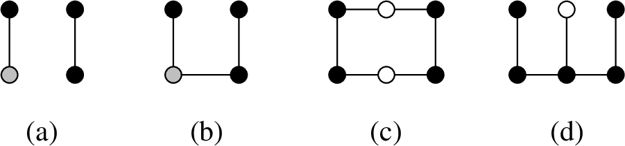
Figure 5 shows some small OTD-admissible bipartite graphs. It is easy to see that \(\gamma^{\rm{OD}}(G)\) and \(\gamma^{\rm{OTD}}(G)\) differ for \(G \in \{2K_2,P_4\}\) and are equal for \(G \in \{C_6, bow\}\). We next exhibit families of bipartite graphs where the OD- and the OTD-numbers differ.
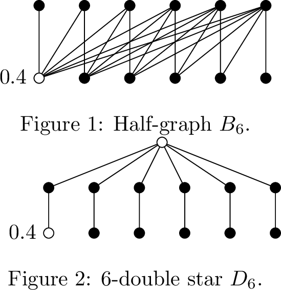
For any integer \(k \geq 1\), the half-graph \(B_k=(U \cup W, E)\) is the bipartite graph with its stable vertex sets \(U = \{u_1, \ldots , u_k\}\) and \(W = \{w_1, \ldots , w_k \}\) and edges \(u_iw_j\) if and only if \(i \leq j\) (see Figure 6). In particular, we have \(B_1=K_2\) and \(B_2=P_4\). Moreover, we clearly see that half-graphs are connected and open-twin-free and hence, are both OD- and OTD-admissible.
In [15] it was shown that the only graphs whose OTD-numbers equal the order of the graph are the disjoint unions of half-graphs. In particular, we have \(\gamma^{\rm{OTD}}(B_k) = |V(B_k)| = 2k\). Now, let \(G = (V,E)\) be a graph that is a disjoint union of half-graphs. By Theorem 3(b), therefore, we have \(\gamma^{\rm{OD}}(G) \geq \gamma^{\rm{OTD}}(G)-1 = |V|-1\). Moreover, by Theorem 2, we have \(\gamma^{\rm{OD}}(G) \leq |V|-1\). Hence, combining the two inequalities, we get the following corollary.
Corollary 4. For a graph \(G=(V,E)\) being the disjoint union of half-graphs, we have \(\gamma^{\rm{OD}}(G) = |V|-1\). In particular, for a half-graph \(B_k\), we have \(\gamma^{\rm{OD}}(B_k) = 2k-1\).
Corollary 4 shows that, on the one hand, disjoint unions of half-graphs are further examples of graphs \(G\) where \(\gamma^{\rm{OD}}(G)\) is larger than the sum of the OD-numbers of its components and, on the other hand, that half-graphs and their disjoint unions are extremal examples of graphs whose OD-numbers also attain the general upper bound in Theorem 2.
Moreover, we note that the upper bound from Theorem 2 does not apply to OD-admissible graphs having an isolated vertex. To see this, consider the graph \(G = B_k + K_1\) for some \(k \geq 1\). By Theorem 3(b), we have \(\gamma^{\rm{OD}}(G) = \gamma^{\rm{OTD}}(B_k) + 1 = 2k+1 = |V(G)|\). As half-graphs and their disjoint unions are the only graphs whose OTD-numbers equal the order of the graph by [15], adding an isolated vertex to them yields the only graphs whose OD-numbers equal the order of the graph.
To give an independent proof for the OD- and OTD-numbers of half-graphs, we next provide their X-clutters.
Lemma 10. For any half-graph \(B_k\) with \(k \geq 2\), we have
\(\mathcal{C}_{{\mathrm{\small OD}}}(B_k) = (2k-2)K_1 \oplus K_{2}\) and \(\gamma^{\rm{OD}}(B_k) = 2k-1\) but
\(\mathcal{C}_{{\mathrm{\small OTD}}}(B_k) = 2kK_1\) and \(\gamma^{\rm{OTD}}(B_k) = 2k\).
Proof. Consider a half-graph \(B_k=(U \cup W, E)\) with its stable vertex sets \(U = \{u_1, \ldots , u_k\}\) and \(W = \{w_1, \ldots , w_k \}\) and edges \(u_iw_j\) if and only if \(i \leq j\) for some \(k \geq 2\). In order to determine \(\mathcal{C}_{{\mathrm{\small X}}}(B_k)\) and \(\gamma^{\rm{X}}(B_k)\) for \({\mathrm{\small X}}\in \{{\mathrm{\small OD}},{\mathrm{\small OTD}}\}\), we first construct the X-hypergraphs. Recall that the following hyperedges are involved: the closed or open neighborhoods
\(N[u_i] = \{u_i\} \cup \{w_i, \ldots, w_k\}\) and \(N(u_i) = \{w_i, \ldots, w_k\}\) for \(1 \leq i \leq k\),
\(N[w_j] = \{u_1, \ldots , u_j\} \cup \{w_j\}\) and \(N(w_j) = \{u_1, \ldots , u_j\}\) for \(1 \leq j \leq k\),
and the symmetric differences of open neighborhoods of distinct vertices
\(\Delta(u_i,u_j) = \{w_i, \ldots, w_{j-1}\}\) for \(1 \leq i < j \leq k\),
\(\Delta(u_i,w_j) = \{w_i, \ldots, w_k\} \cup \{u_1, \ldots , u_j\}\) for \(1 \leq i,j \leq k\),
\(\Delta(w_i,w_j) = \{u_{1+1}, \ldots , u_j\}\) for \(1 \leq i < j \leq k\).
In particular, we see that
\(\Delta(u_i,u_{1+1}) = \{w_i\}\) for \(1 \leq i < k\),
\(\Delta(w_i,w_{1+1}) = \{u_{1+1}\}\) for \(1 \leq i < k\)
belong to \(\mathcal{F}^1_{{\mathrm{\small X}}}(B_k)\) for \({\mathrm{\small X}}\in \{{\mathrm{\small OD}},{\mathrm{\small OTD}}\}\). Noting further that \(N(u_k) = \{w_k\}\) and \(N(w_1) = \{u_1\}\) holds implies \(\mathcal{F}^1_{{\mathrm{\small OTD}}}(B_k) = U \cup W\) and thus \(\mathcal{C}_{{\mathrm{\small OTD}}}(B_k) = 2kK_1\) and \(\gamma^{\rm{OTD}}(B_k) = 2k\). On the other hand, it is easy to see that \(\Delta(u_k,w_1) = \{w_k,u_1\}\) is the only hyperedge in \(\mathcal{F}^2_{{\mathrm{\small OD}}}(B_k)\), thus \(\mathcal{C}_{{\mathrm{\small OD}}}(B_k) = (2k-2)K_1 \oplus K_{2}\) and \(\gamma^{\rm{OD}}(B_k) = 2k-1\) follows. ◻
A \(k\)-double star \(D_k=(U \cup W, E)\) is the bipartite graph with its stable vertex sets \(U = \{u_0,u_1, \ldots , u_k\}\) and \(W = \{w_1, \ldots , w_k \}\) and edges \(u_iw_i\) and \(u_0w_i\) for all \(w_i \in W\) (see Figure [fig:double95star]). Then, we have \(D_1=P_3\) and \(D_2=P_5\). Moreover, we clearly see that \(k\)-double stars with \(k \geq 2\) are connected and open-twin-free and hence, are both OD- and OTD-admissible. As the next lemma shows, \(k\)-double stars also provide examples of bipartite graphs where the OD- and the OTD-numbers differ.
Lemma 11. For a \(k\)-double star \(D_k\) with \(k \geq 3\), \(\mathcal{C}_{{\mathrm{\small OD}}}(D_k)\) is composed of
\(\{u_i,w_i\}\) for \(1 \leq i \leq k\),
\(\{u_0,u_j,w_i\}\) for \(1 \leq i,j \leq k\) for \(i \neq j\),
\(\{u_i,u_j\}\) and \(\{w_i,w_j\}\) for \(1 \leq i < j \leq k\),
and thus \(\gamma^{\rm{OD}}(D_k) = 2k-1\) follows, whereas \(\mathcal{C}_{{\mathrm{\small OTD}}}(D_k)\) is composed of
\(\{w_i\}\) and \(\{u_0,u_i\}\) for \(1 \leq i < k\),
\(\{u_i,u_j\}\) for \(1 \leq i < j \leq k\).
and \(\gamma^{\rm{OTD}}(D_k) = 2k\) holds.
Proof. Consider a \(k\)-double star \(D_k=(U \cup W, E)\) with vertex sets \(U = \{u_0,u_1, \ldots , u_k\}\) and \(W = \{w_1, \ldots , w_k \}\) and edges \(u_i w_i\) and \(u_0 w_i\) for all \(w_i \in W\) for some \(k \geq 3\). In order to determine \(\mathcal{C}_{{\mathrm{\small X}}}(D_k)\) and \(\gamma^{\rm{X}}(D_k)\) for \({\mathrm{\small X}}\in \{{\mathrm{\small OD}},{\mathrm{\small OTD}}\}\), we first construct the X-hypergraphs. Recall that the following hyperedges are involved: the closed or open neighborhoods
\(N[u_0] = \{u_0\} \cup W\) and \(N(u_0) = W\),
\(N[u_i] = \{u_i,w_i\}\) and \(N(u_i) = \{w_i\}\) for \(1 \leq i \leq k\),
\(N[w_i] = \{u_0,u_i,w_i\}\) and \(N(w_i) = \{u_0,u_i\}\) for \(1 \leq i \leq k\),
and the symmetric differences of open neighborhoods of distinct vertices
\(\Delta(u_0,u_i) = W \setminus \{w_i\}\) for \(1 \leq i \leq k\),
\(\Delta(u_0,w_i) = W \cup \{u_0,u_i\}\) for \(1 \leq i \leq k\),
\(\Delta(u_i,u_j) = \{w_i,w_j\}\) for \(1 \leq i < j \leq k\),
\(\Delta(u_i,w_j) = \{u_0,u_j,w_i\}\) for \(1 \leq i,j \leq k\),
\(\Delta(w_i,w_j) = \{u_i,u_j\}\) for \(1 \leq i < j \leq k\).
The OD-hypergraph involves the closed neighborhoods and all symmetric differences, including
\(N[u_i] = \{u_i,w_i\}\) for \(1 \leq i \leq k\),
\(\Delta(u_i,u_j) = \{w_i,w_j\}\) for \(1 \leq i < j \leq k\),
\(\Delta(u_i,w_j) = \{u_0,u_j,w_i\}\) for \(1 \leq i,j \leq k\) for \(i \neq j\),
\(\Delta(w_i,w_j) = \{u_i,u_j\}\) for \(1 \leq i < j \leq k\),
which implies that all other hyperedges are redundant for any \(k \geq 3\). Analyzing the hyperedges remaining in \(\mathcal{C}_{{\mathrm{\small OD}}}(D_k)\) shows that \((U \setminus \{u_i\}) \cup (W \setminus \{w_j\})\) for \(0 \leq i \leq k\), \(1 \leq j \leq k\) and \(i \neq j\) as well as \((U \setminus \{u_0,u_i\}) \cup W\) for \(1 \leq i \leq k\) are the only minimum OD-codes of \(D_k\) and thus \(\gamma^{\rm{OD}}(D_k) = 2k-1\) follows.
The OTD-hypergraph involves the open neighborhoods and all symmetric differences, including
\(N(u_i) = \{w_i\}\) for \(1 \leq i \leq k\),
\(N(w_i) = \{u_0,u_i\}\) for \(1 \leq i \leq k\),
\(\Delta(w_i,w_j) = \{u_i,u_j\}\) for \(1 \leq i < j \leq k\),
which implies that all other hyperedges are redundant for any \(k \geq 3\). Analyzing the hyperedges remaining in \(\mathcal{C}_{{\mathrm{\small OTD}}}(D_k) = kK_1 \oplus K_{k+1}\) shows that \((U \setminus \{u_i\}) \cup W\) for \(0 \leq i \leq k\) are the only minimum OTD-codes of \(D_k\) and \(\gamma^{\rm{OTD}}(D_k) = 2k\) holds. ◻
4.4 Families of split graphs↩︎
In order to study OD-codes of split graphs and compare them with the OTD-codes, we restrict ourselves to split graphs \(G\) without open twins and isolated vertices. This further implies that \(G\) is connected and \(Q\) non-empty (as, otherwise, every component not containing the clique \(Q\) needs to be an isolated vertex from \(S\), contradicting our assumptions). Figure 7 shows some small OTD-admissible split graphs. It is easy to see that \(\gamma^{\rm{OD}}(G)\) and \(\gamma^{\rm{OTD}}(G)\) differ for \(G \in \{P_4, gem\}\) and are equal for \(G \in \{net, sun\}\).
We next examine OD-codes in two families of split graphs for which the exact OTD-numbers are known from [11]. A headless spider is a split graph with \(Q = \{q_1, \ldots, q_k\}\) and \(S = \{s_1, \ldots, s_k\}\). In addition, a headless spider is thin (respectively, thick) if \(s_i\) is adjacent to \(q_j\) if and only if \(i = j\) (respectively, \(i \neq j\)). By definition, it is clear that the complement of a thin headless spider \(H_k\) is a thick headless spider \(\overline{H}_k\), and vice-versa. We have \(H_2 = \overline{H}_2 = P_4\), the two headless spiders \(H_3 = net\) and \(\overline{H}_3 = sun\) are depicted in Figures 7 (c) and 7 (d), respectively. Moreover, it is easy to check that thin and thick headless spiders have no twins.
In [11], it was shown that \(\gamma^{\rm{OTD}}(H_k) = k\) for \(k \geq 3\) and \(\gamma^{\rm{OTD}}(\overline{H}_k) = k+1\) for \(k \geq 3\). We next analyse the OD-numbers of thin and thick headless spiders.
Lemma 12. For a thick headless spider \(\overline{H}_k=(Q \cup S, E)\) with \(k \geq 3\), the OD-clutter is composed of the symmetric differences of non-adjacent vertices
\(N(q_i) \Delta N(s_i) = S \setminus \{s_i\}\) for all \(i \in \{1, \ldots, k\}\),
\(N(s_i) \Delta N(s_j) = \{q_i,q_j\}\) for \(i \in \{1, \ldots, k\}\), \(j \in \{1, \ldots, k\} \setminus \{i\}\)
and we thus have \(\mathcal{C}(\overline{H}_k) = {\cal{R}}_{|S|}^{|S|-1} \cup {\cal{R}}_{|Q|}^2\) and \(\gamma^{\rm{OD}}(\overline{H}_k) = k+1\).
Proof. Consider a thick headless spider \(\overline{H}_k=(Q \cup S, E)\) with \(k \geq 3\). \(\mathcal{H}_{{\mathrm{\small OD}}}(\overline{H}_k)\) is composed of the closed neighborhoods
\(N[s_i] = Q \setminus \{q_i\} \cup \{s_i\}\) for all \(s_i \in S\),
\(N[q_i] = Q \cup \{s_i\}\) for all \(q_i \in Q\)
and the symmetric differences
\(\Delta(s_i,s_j) = \{q_i,q_j\}\) for all distinct \(s_i,s_j \in S\),
\(\Delta(q_i,q_j) = \{q_i,q_j\} \cup \{s_i,s_j\}\) for all distinct \(q_i,q_j \in C\),
\(\Delta(q_i,s_j) = \begin{cases} S \setminus \{s_i\}, &if i=j; \\ \{q_i,q_j\} \cup S \setminus \{s_i\}, &if i \neq j.\\ \end{cases}\)
This shows that all neighborhoods are redundant as well as all \(\Delta(q_i,q_j)\) and \(\Delta(q_i,s_j)\) with \(i \neq j\) so that only \(\Delta(s_i,s_j)\) and \(\Delta(q_i,s_i)\) belong to \(\mathcal{C}_{{\mathrm{\small OD}}}(\overline{H}_k)\). Hence, we obtained \(\mathcal{C}_{{\mathrm{\small OD}}}(\overline{H}_k) = {\cal{R}}_{|S|}^{|S|-1} \cup {\cal{R}}_{|Q|}^2\). Finally, this implies \(\gamma^{\rm{OD}}(\overline{H}_k) = 2 + (k-1) = k+1\) by the result from [31]. ◻
Lemma 13. For a thin headless spider \(H_k=(Q \cup S, E)\) with \(k \geq 4\), the OD-clutter is composed of
\(N[s_i] = \{q_i,s_i\}\) for all \(i \in \{1, \ldots, k\}\),
\(N(s_i) \Delta N(s_j) = \{q_i,q_j\}\) for \(i \in \{1, \ldots, k\}\), \(j \in \{1, \ldots, k\} \setminus \{i\}\)
and we thus have \(\mathcal{C}_{{\mathrm{\small OD}}}(H_k) = H_k\) and \(\gamma^{\rm{OD}}(H_k) = k\).
Proof. Consider a thin headless spider \(H_k=(Q \cup S, E)\) with \(k \geq 4\). \(\mathcal{H}_{{\mathrm{\small OD}}}(H_k)\) is composed of the closed neighborhoods
\(N[s_i] = \{s_i,q_i\}\) for all \(s_i \in S\),
\(N[q_i] = Q \cup \{s_i\}\) for all \(q_i \in Q\)
and the symmetric differences
\(\Delta(s_i,s_j) = \{q_i,q_j\}\) for all distinct \(s_i,s_j \in S\),
\(\Delta(q_i,q_j) = \{q_i,q_j\} \cup \{s_i,s_j\}\) for all distinct \(q_i,q_j \in Q\),
\(\Delta(q_i,s_j) = \begin{cases} Q \cup \{s_i\}, &if i=j; \\ (Q \setminus \{q_i,q_j\}) \cup \{s_i\}, &if i \neq j.\\ \end{cases}\)
We deduce that in \(\mathcal{C}_{{\mathrm{\small OD}}}(H_k)\) with \(k \geq 4\) only
\(N[s_i] = \{s_i,q_i\}\) for all \(s_i \in S\),
\(\Delta(s_i,s_j) = \{q_i,q_j\}\) for all distinct \(s_i,s_j \in S\)
remain and thus \(\mathcal{C}_{{\mathrm{\small OD}}}(H_k) = H_k\) follows. Hence \(\mathcal{C}_{{\mathrm{\small OD}}}(H_k)\) contains the disjoint hyperedges \(\{q_i,s_i\}\) for \(1 \leq i \leq k\) which shows \(\gamma^{\rm{OD}}(H_k) \geq k\). On the other hand, \(Q\) is clearly a cover of \(\mathcal{C}_{{\mathrm{\small OD}}}(H_k) = H_k\) of cardinality \(k\), which finally implies \(\gamma^{\rm{OD}}(H_k) = k\). ◻
Moreover, it is easy to see that \(\gamma^{\rm{OD}}(H_3) = 3\) (see Figure 7 (c)), hence the two lemmas combined with the results from [11] show that for thin and thick headless spiders \(H_k\) and \(\overline{H}_k\), respectively, the OD- and the OTD-numbers are equal for all \(k \geq 3\).
In [24], the question was raised whether there also exist infinite families of open twin-free split graphs where the OD- and the OTD-numbers differ. To answer this question, we consider the following extension of thin headless spiders. Consider a split graph \(G=(Q \cup S, E)\) with \(Q = \{q_1, \ldots, q_k\}\) and \(S = \{s_0,s_1, \ldots, s_k\}\), where \(s_i\) is adjacent to \(q_i\) for all \(1 \leq i \leq k\) and \(s_0\) is adjacent to \(\{q_1, \ldots, q_{k-1}\}\). By definition, it is clear that \(G[Q \cup S\setminus\{s_0\}]\) is isomorphic to the thin headless spider \(H_k\). Hence, we call such split graphs extended thin spiders \(E_k\).
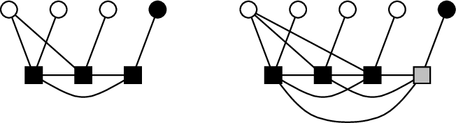
It is easy to see that for \(k \geq 3\), extended thin spiders \(E_k\) have neither isolated vertices nor open twins, see Figure 8 for illustration. We can show:
Lemma 14. For an extended thin spider \(E_k=(Q \cup S, E)\) with \(k \geq 4\), the
OD-clutter is composed of \(\{s_k\}\), \(\{q_i,s_i\}\) for all \(1 \leq i < k\), and \(\{q_i,q_j\}\) for all \(1 \leq i < j \leq k\) and we thus have \(\gamma^{\rm{OD}}(E_k) = k\);
OTD-clutter is composed of \(\{s_k\}\) and \(\{q_i\}\) for \(1 \leq i \leq k\) and we have \(\gamma^{\rm{OTD}}(E_k) = k+1\).
Proof. Consider an extended thin spider \(E_k=(Q \cup S, E)\) with \(k \geq 4\). In order to determine \(\mathcal{C}_{{\mathrm{\small X}}}(E_k)\) and \(\gamma^{\rm{X}}(E_k)\) for \({\mathrm{\small X}}\in \{{\mathrm{\small OD}},{\mathrm{\small OTD}}\}\), we first construct the X-hypergraphs. Recall that the following hyperedges are involved: the closed or open neighborhoods
\(N[s_0] = \{s_0\} \cup (Q \setminus\{q_k\})\) and \(N(s_0) =Q \setminus\{q_k\}\),
\(N[s_i] = \{s_i,q_i\}\) and \(N(s_i) =\{q_i\}\) for \(1 \leq i \leq k\),
\(N[q_i] = Q \cup \{s_0,s_i\}\) and \(N(q_i) =(Q \setminus\{q_i\}) \cup \{s_0,s_i\}\) for \(1 \leq i < k\),
\(N[q_k] = Q \cup \{s_k\}\) and \(N(q_k) =(Q \setminus\{q_k\}) \cup \{s_k\}\),
and the symmetric differences of open neighborhoods of distinct vertices
\(\Delta(s_0,s_i) = Q \setminus\{q_i,q_k\}\) for \(1 \leq i < k\),
\(\Delta(s_0,s_k) = Q\),
\(\Delta(s_0,q_i) = \{q_i,q_k\} \cup \{s_0,s_i\}\) for \(1 \leq i < k\),
\(\Delta(s_0,q_k) = \{s_k\}\),
\(\Delta(s_i,s_j) = \{q_i,q_j\}\) for \(1 \leq i < j \leq k\),
\(\Delta(s_i,q_i) = Q \cup \{s_0,s_i\}\) for \(1 \leq i < k\),
\(\Delta(s_k,q_k) = Q \cup \{s_k\}\),
\(\Delta(s_i,q_j) = (Q \setminus \{q_i,q_j\}) \cup \{s_0,s_j\}\) for \(1 \leq j < i \leq k\),
\(\Delta(s_i,q_k) = (Q \setminus \{q_i,q_k\}) \cup \{s_k\}\) for \(1 \leq i < k\),
\(\Delta(q_i,q_j) = \{q_i,q_j\} \cup \{s_i,s_j\}\) for \(1 \leq j < i \leq k\),
\(\Delta(q_i,q_k) = \{q_i,q_k\} \cup \{s_0,s_i,s_k\}\) for \(1 \leq i < k\).
The OD-hypergraph involves the closed neighborhoods and all symmetric differences, including
\(\Delta(s_0,q_k) = \{s_k\}\),
\(N[s_i] = \{s_i,q_i\}\) for \(1 \leq i < k\), and
\(\Delta(s_i,s_j) = \{q_i,q_j\}\) for \(1 \leq i < j \leq k\),
which implies that all other hyperedges are redundant and \(V^0_{{\mathrm{\small OD}}}(E_k)=\{s_0\}\). The subset \(\{s_k\}\) and \(\{s_i,q_i\}\) for \(1 \leq i < k\) of disjoint hyperedges shows \(\gamma^{\rm{OD}}(E_k) \geq k\). On the other hand, \(Q \setminus \{q_k\} \cup \{s_k\}\) is clearly a cover of \(\mathcal{C}_{{\mathrm{\small OD}}}(E_k)\) of cardinality \(k\), which finally implies \(\gamma^{\rm{OD}}(E_k) = k\).
The OTD-hypergraph involves the open neighborhoods and all symmetric differences, including
\(N(s_i) =\{q_i\}\) for \(1 \leq i \leq k\),
\(\Delta(s_0,q_k) = \{s_k\}\),
which implies that all other hyperedges are redundant and \(V^0_{{\mathrm{\small OTD}}}(E_k)=S \setminus \{s_k\}\). This clearly shows that \(Q \cup \{s_k\}\) is the only minimum cover of \(\mathcal{C}_{{\mathrm{\small OTD}}}(E_k)\) and we have \(\gamma^{\rm{OTD}}(E_k) = k+1\). ◻
4.5 Families of thin suns↩︎
The result on thin headless spiders can be further generalized to thin suns. A sun is a graph \(G=(C\cup S,E)\) whose vertex set can be partitioned into \(S\) and \(C\), where, for an integer \(k \geq 3\), the set \(S = \{s_1, \ldots, s_k\}\) is a stable set and \(C = \{c_1, \ldots, c_k\}\) is a (not necessarily chordless) cycle. A thin sun \(T_k=(C\cup S,E)\) is a sun where \(s_i\) is adjacent to \(c_j\) if and only if \(i = j\). Therefore, thin headless spiders are special thin suns where all chords of the cycle \(C\) are present (such that \(C\) induces a clique). Other special cases of thin suns are sunlets where no chords of the cycle \(C\) are present (such that \(C\) induces a hole). For illustration, for \(k=3\), the (only) thin sun \(T_3\) equals the thin headless spider \(H_3\) (see Figure 7 (c)); for \(k=4\), the three possible thin suns \(T_4\) are depicted in Figure 9. We further note that thin suns have neither isolated vertices nor open twins. We first determine the OD-clutter of thin suns.
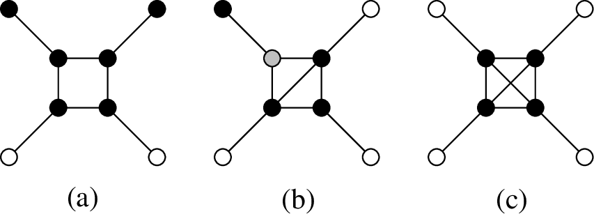
Lemma 15. For a thin sun \(T_k=(C \cup S, E)\) with \(k \geq 4\), the OD-clutter \(\mathcal{C}_{{\mathrm{\small OD}}}(T_k)\) is composed of
\(N[s_i] = \{s_i,c_i\}\) for all \(s_i \in S\),
\(\Delta(s_i,s_j) = \{c_i,c_j\}\) for all distinct \(s_i,s_j \in S\),
\(\Delta(c_i,c_j) = \begin{cases} \{s_i,s_j\}, &if c_i, c_j are open C-twins; \\ \{s_i,s_j,c_{\ell}\}, &if c_i, c_j non-adjacent and \{c_{\ell}\} = N_C(c_i) \Delta N_C(c_j), \end{cases}\)
\(\Delta(c_i,s_j) = \{s_i,c_{\ell}\}\) if \(c_i, c_j\) are adjacent and \(\{c_{\ell}\} = N_C(c_i) \setminus \{c_{j}\}\), \(\ell \neq i,j\).
Proof. \(\mathcal{H}_{{\mathrm{\small OD}}}(T_k)\) is composed of the closed neighborhoods
\(N[s_i] = \{s_i,c_i\}\) for all \(s_i \in S\),
\(N[c_i] = N_C[c_i] \cup \{s_i\}\) for all \(c_i \in C\)
and the symmetric differences
\(\Delta(s_i,s_j) = \{c_i,c_j\}\) for all distinct \(s_i,s_j \in S\),
\(\Delta(c_i,c_j) = (N_C(c_i) \Delta N_C(c_j)) \cup \{s_i,s_j\}\) for all distinct \(c_i,c_j \in C\),
\(\Delta(c_i,s_j) = \begin{cases} N[c_i], &if i=j; \\ (N_C(c_i) \cup \{s_i\}) \Delta \{c_j\}, &if i \neq j.\\ \end{cases}\)
This shows that \(N[s_i]\) and \(\Delta(s_i,s_j)\) belong to \(\mathcal{C}_{{\mathrm{\small OD}}}(T_k)\) which further implies that the following hyperedges from \(\mathcal{H}_{OD}(T_k)\) are redundant:
\(N[c_i] = N_C[c_i] \cup \{s_i\}\) for all \(c_i \in C\),
\(\Delta(c_i,c_j)\) if \(|N_C(c_i) \Delta N_C(c_j)| \geq 2\),
\(\Delta(c_i,s_j)\) if \(c_i, c_j\) are non-adjacent or if \(c_i, c_j\) are adjacent but \(|N_C(c_i)| \geq 3\).
In the remaining cases, \(\Delta(c_i,c_j)\) and \(\Delta(c_i,s_j)\) belong to \(\mathcal{C}_{{\mathrm{\small OD}}}(T_k)\). ◻
We call two vertices \(c_i\) and \(c_j\) of a thin sun \(T_k=(C\cup S,E)\) open \(C\)-twins if \(c_i\) and \(c_j\) are non-adjacent and \(N_C(c_i) = N_C(c_j)\), where \(N_C(v) = N(v) \cap C\). For instance, the sunlet in Figure 9 (a) and the thin sun in Figure 9 (b) have open \(C\)-twins, whereas the thin headless spider in Figure 9 (c) does not.
In [11], it was shown that for a thin sun \(T_k\) with \(k \geq 4\) and without open \(C\)-twins, the set \(C\) is the unique minimum OTD-code of \(T_k\) and thus, we have \(\gamma^{\rm{OTD}}(T_k) = k\). Now, with regards to OD-numbers of thin suns, we show the following.
Lemma 16. For a thin sun \(T_k=(C \cup S, E)\) with \(k \geq 4\) and without open \(C\)-twins, \(C\) is a minimum \({\mathrm{\small OD}}\)-code and hence, we have \(\gamma^{\rm{OD}}(T_k)=|C|=k\).
Proof. Consider a thin sun \(T_k=(C \cup S, E)\) with \(k \geq 4\) and without open \(C\)-twins. By Lemma 15, the OD-clutter \(\mathcal{C}_{{\mathrm{\small OD}}}(T_k)\) contains \(\{s_i,c_i\}\) for all \(s_i \in S\), which implies the lower bound \(\gamma^{\rm{OD}}(T_k) \geq k\). On the other hand, it is easy to verify that, by Lemma 15, all hyperedges of the OD-clutter \(\mathcal{C}_{{\mathrm{\small OD}}}(T_k)\) have a nonempty intersection with \(C\) (when \(T_k\) has no open \(C\)-twins) so that \(C\) is a cover of \(\mathcal{C}_{{\mathrm{\small OD}}}(T_k)\) of cardinality \(k\). Hence, \(C\) is a minimum OD-code and the assertion \(\gamma^{{\mathrm{\small OD}}}(T_k)=|C|=k\) follows. ◻
Therefore, thin suns without open \(C\)-twins are examples of graphs where the OD- and the OTD-number are equal. This applies in particular to sunlets and to thin headless spiders. However, for thin suns \(T_k\) with open \(C\)-twins, \(\gamma^{\rm{OD}}(T_k)\) and \(\gamma^{\rm{OTD}}(T_k)\) may differ. For instance, for the thin sun \(T_4\) depicted in Fig. 9 (b), it can be checked that \(\gamma^{\rm{OD}}(T_4) = 4 < 5 = \gamma^{\rm{OTD}}(T_4)\). We call a thin sun \(T_k=(C \cup S, E)\) almost complete if \(k = 2\ell\) and \(c_i\) is non-adjacent to \(c_{i + \ell}\) but is adjacent to all other \(c_j \in C\). For instance, the sunlet in Fig. 9 (a) is almost complete. We can show:
Lemma 17. For an almost complete thin sun \(T_{2\ell}\) with \(\ell \geq 3\), we have \(\gamma^{\rm{OD}}(T_{2\ell}) = 3\ell - 1\) and \(\gamma^{\rm{OTD}}(T_{2\ell}) = 3\ell\).
Proof. Consider an almost complete thin sun \(T_{2\ell}\) with \(\ell \geq 3\) where \(c_i,c_{i+\ell}\) form open \(C\)-twins. By Lemma 15, the OD-clutter \(\mathcal{C}_{{\mathrm{\small OD}}}(T_{2\ell})\) is composed of
\(N[s_i] = \{s_i,c_i\}\) for all \(s_i \in S\),
\(\Delta(s_i,s_j) = \{c_i,c_j\}\) for all distinct \(s_i,s_j \in S\),
\(\Delta(c_i,c_{i+\ell}) = \{s_i,s_{i+\ell}\}\) for all \(c_i \in C\).
Hence, every cover of \(\mathcal{C}_{{\mathrm{\small OD}}}(T_{2\ell})\) has to contain at least all but one vertex from \(C\) and one of \(\{s_i,s_{i+\ell}\}\) for all \(1 \leq i \leq \ell\), showing that \(\gamma^{\rm{OD}}(T_{2\ell}) \geq 3\ell - 1\). We next observe that \(V' = \{s_1, \ldots, s_{\ell}\} \cup C \setminus \{c_j\}\) for some \(j \in \{1, \ldots, {\ell}\}\) is a cover of \(\mathcal{C}_{{\mathrm{\small OD}}}(T_{2\ell})\). Indeed, \(V'\) meets all
\(N[s_i] = \{s_i,c_i\}\) in \(s_i\) for \(1 \leq i \leq \ell\) and in \(c_i\) for \(\ell+1 \leq i \leq 2\ell\),
\(\Delta(s_i,s_j) = \{c_i,c_j\}\) as \(V'\) contains all but one vertex from \(C\),
\(\Delta(c_i,c_{i+\ell}) = \{s_i,s_{i+\ell}\}\) in \(s_i\) for \(1 \leq i \leq \ell\).
Hence, \(V'\) is an OD-code of \(T_{2\ell}\) and \(\gamma^{\rm{OD}}(T_{2\ell}) = 3\ell - 1\) follows. Furthermore, from [11] we deduce that the OTD-clutter \(\mathcal{C}_{{\mathrm{\small OTD}}}(T_{2\ell})\) is composed of
\(N(s_i) = \{c_i\}\) for all \(s_i \in S\),
\(\Delta(c_i,c_{i+\ell}) = \{s_i,s_{i+\ell}\}\) for all \(c_i \in C\).
For an almost complete thin sun \(T_{2\ell}\) with \(\ell \geq 3\), this implies that \(C \cup \{s_1, \ldots, s_{\ell}\}\) is a minimum OTD-code of \(T_{2\ell}\) and, hence, \(\gamma^{\rm{OTD}}(T_{2\ell}) = 3\ell\) follows. ◻
Hence, there exist infinitely many thin suns with open \(C\)-twins for which the OD- and the OTD-numbers differ.
5 Polyhedra associated with OD-codes↩︎
As polyhedral methods turned out to be successful for many NP-hard combinatorial optimization problems in the literature, it was suggested in e.g. [11], [27] to apply such techniques to identification problems. For that, the reformulation of the studied X-problem in a graph \(G\) as covering problem in the hypergraph \(\mathcal{H}_X(G)\) was used. In fact, the incidence matrix of \(\mathcal{H}_X(G)\) defines the constraint system of the resulting covering problem. We next provide some preliminaries and then study OD-codes in this context.
5.0.0.1 About covering polyhedra.
Consider a \(0/1\)-matrix \(M\) with \(n\) columns. A cover of \(M\) is a vector \(\mathbf{x} \in \mathbf{Z}_+^n\) such that \(M \mathbf{x} \geq \mathbf{1}\) holds where \(\mathbf{1}\) is the vector having \(1\)-entries only (note that a minimum cover \(\mathbf{x}\) has \(0/1\)-entries only). The covering number of \(M\) can be calculated by \[\begin{array}{rcl} \displaystyle \tau(M) = \min \mathbf{1}^T\mathbf{x} \;& & \\ M \;\mathbf{x} \;& \geq & \mathbf{1} \\ \mathbf{x} \;& \in & \mathbf{Z}_+^n. \\ \end{array}\] The covering polyhedron of \(M\) is defined by \(P(M)=conv\left\{\mathbf{x} \in \mathbf{Z}_+^n: M \mathbf{x} \geq \mathbf{1} \right\}\) and encodes the convex hull of all covers of \(M\). The following properties of general covering polyhedra are known from [32]:
Theorem 9 ([32]). Consider a \(0/1\)-matrix \(M\) with \(n\) columns and the covering polyhedron \(P(M)\).
\(P(M)\) has dimension \(n\) if and only if \(M\) has at least two ones per row.
The only facet-defining inequalities of \(P(M)\) with integer coefficients and right hand side equal to one are those of the constraint system \(M \mathbf{x} \geq \mathbf{1}\).
The linear relaxation \(Q(M)=\left\{\mathbf{x} \in \mathbf{R}_+^n: M \mathbf{x} \geq \mathbf{1} \right\}\) of \(P(M)\) satisfies \(P(M) \subseteq Q(M)\) in general, and \(M\) is called ideal if \(P(M) = Q(M)\) holds. For all non-ideal matrices \(M\), further constraints (with right hand side \(> 1\)) have to be added to the system \(M \mathbf{x} \geq \mathbf{1}\) in order to describe \(P(M)\) using real variables instead of integral ones.
One type of such constraints can be obtained as follows. For a \(0/1\)-matrix \(M\) with \(n\) columns and a column subset \(J \subseteq \{1, \ldots, n\}\), a minor \(M' = M \setminus U\) is obtained by
deleting a column \(j \in J\) (that is, removing from \(M\) column \(j\) and all rows having a 1-entry in column \(j\), which corresponds to setting \(x_j = 1\) in the system \(M \mathbf{x} \geq \mathbf{1}\)) or
contracting a column \(j \in J\) (that is, removing from \(M\) column \(j\) and all rows \(\mathbf{y}\) that became redundant as there is now another row \(\mathbf{y}'\) with \(\mathbf{y}' \leq \mathbf{y}\), which corresponds to setting \(x_j = 0\) in the system \(M \mathbf{x} \geq \mathbf{1}\))
in any order. For such a minor \(M' = M \setminus J\), the rank-constraint associated with \(M'\) is \[\label{eq95rank} x(M') = \sum_{i \in \{1, \ldots, n\} \setminus J}x_i \geq \tau(M')\tag{1}\] and we have the following according to [33].
Theorem 10 ([33]). Let \(M\) be a \(0/1\)-matrix and \(M'\) be some minor of \(M\). If the rank-constraint (1 ) associated with \(M'\) is a facet of \(P(M')\), then it is also a facet of \(P(M)\).
Hence, essential constraints associated with minors \(M'\) remain essential for the covering polyhedron of the whole matrix \(M\).
For any hypergraph \(\mathcal{H} = (V, \mathcal{E})\), let \(M(\mathcal{H})\) denote its incidence matrix encoding row-wise its hyperedges \(F\) (that is, the row of \(M(\mathcal{H})\) corresponding to \(F\) is a \(0/1\)-vector of length \(|V|\) having a \(1\)-entry if \(v \in F\) and a \(0\)-entry otherwise). Note that \(\tau(\mathcal{H}) = \tau(M(\mathcal{H}))\) clearly holds.
The covering polyhedra associated with complete \(q\)-roses of order \(n\) were studied in [27], [31]. In [31], it has been proved that the rank-constraint associated with \(M({\cal{R}}_n^q)\) defines a facet of \(P(M({\cal{R}}_n^q))\). In [27], it was shown that any minor of \(M({\cal{R}}_n^q)\) corresponds to a complete \(q'\)-rose of order \(n'\) with \(q' \leq q\) and \(n' \leq n\), and that no other constraints than rank-constraint associated with such minors define facets:
Theorem 11 ([27]). The covering polyhedron of the incidence matrix of a complete \(q\)-rose \({\cal{R}}_n^q\) of order \(n\) is given by the non-negativity constraints and \[x(V') = \sum_{v \in V'}x_v \geq |V'|-q +1\] for all subsets \(V' \subseteq \{1,\ldots,n\}\) with \(|V'| \in \{q,\ldots,n\}\).
Note that this also reproves the result from [31] showing that \(\tau({\cal{R}}_n^q)=n-q+1\) holds.
5.1 Polyhedra associated with OD-codes↩︎
Following a similar approach as in e.g. [11], [27] for X-problems with \({\mathrm{\small X}}\in \{{\mathrm{\small ID}},{\mathrm{\small LD}},{\mathrm{\small LTD}},{\mathrm{\small OTD}}\}\), we study here polyhedra associated with OD-codes. Due to \(\gamma^{\rm{OD}}(G)=\tau(\mathcal{H}_{{\mathrm{\small OD}}}(G)) = \tau(\mathcal{C}_{{\mathrm{\small OD}}}(G))\), we can determine a minimum OD-code in a graph \(G=(V,E)\) by solving the following covering problem \[\begin{array}{rcl} \displaystyle \min \mathbf{1}^T\mathbf{x} \;& & \\ M_{{\mathrm{\small OD}}}(G) \;\mathbf{x} \;& \geq & \mathbf{1} \\ \mathbf{x} \;& \in & \mathbf{Z}_+^{|V|} \\ \end{array}\] where \(M_{{\mathrm{\small OD}}}(G)\) is the incidence matrix of the OD-clutter \(\mathcal{C}_{{\mathrm{\small OD}}}(G)\). Accordingly, the OD-polyhedron of a graph \(G\) is defined by \[P_{{\mathrm{\small OD}}}(G)= P(M_{{\mathrm{\small OD}}}(G)) = conv\{\mathbf{x} \in \mathbf{Z}_+^{|V|} : M_{{\mathrm{\small OD}}}(G)\;\mathbf{x} \geq \mathbf{1}\}.\] Based on Theorem 9 from [32] on general covering polyhedra, we prove the following.
Theorem 12. Let \(G=(V,E)\) be an OD-admissible graph. \(P_{{\mathrm{\small OD}}}(G)\) has
the equation \(x_v = 1\) for all forced vertices \(v \in \mathcal{F}^1_{{\mathrm{\small OD}}}(G)\);
a non-negativity constraint \(x_v \geq 0\) for all vertices \(v \not\in \mathcal{F}^1_{{\mathrm{\small OD}}}(G)\); and
a facet \(\sum_{v \in F}x_v \geq 1\) for all hyperedges \(F\) of \(\mathcal{C}_{{\mathrm{\small OD}}}(G)\) with \(F \in \mathcal{F}^2_{{\mathrm{\small OD}}}(G)\).
Proof. Let \(G=(V,E)\) be an OD-admissible graph. By the definition of \(\mathcal{F}^1_{{\mathrm{\small OD}}}(G)\), we clearly have \(x_v = 1\) for all forced vertices \(v \in \mathcal{F}^1_{{\mathrm{\small OD}}}(G)\). This makes the non-negativity constraints for forced vertices redundant so that only \(x_v \geq 0\) for all vertices \(v \not\in \mathcal{F}^1_{{\mathrm{\small OD}}}(G)\) remain.
From Theorem 9 by [32] it is further known that the only facet-defining (i.e. essential) inequalities of a covering polyhedron \(P(M)\) with integer coefficients and right hand side equal to \(1\) are those of the defining system \(M \mathbf{x} \geq \mathbf{1}\). Hence, for \(M = M_{{\mathrm{\small OD}}}(G)\), all constraints \(\sum_{v \in F}x_v \geq 1\) for all hyperedges \(F \in \mathcal{F}^2_{{\mathrm{\small OD}}}(G)\) are facet-defining for \(P_{{\mathrm{\small OD}}}(G)\). ◻
To illustrate these general properties, consider a half-graph \(B_k=(U \cup W, E)\) for some \(k \geq 2\) and recall from Lemma 10 that \(\mathcal{F}^1_{{\mathrm{\small OD}}}(B_k) = (U \setminus \{u_1\}) \cup (W \setminus \{w_k\})\) holds and that \(\{u_1,w_k\}\) is the only hyperedge in \(\mathcal{F}^2_{{\mathrm{\small OD}}}(B_k)\). According to Theorem 12, \(P_{{\mathrm{\small OD}}}(B_k)\) thus has
the equation \(x_v = 1\) for all forced vertices \(v \in \mathcal{F}^1_{{\mathrm{\small OD}}}(B_k) = (U \setminus \{u_1\}) \cup (W \setminus \{w_k\})\);
two non-negativity constraints \(x_{u_1} \geq 0\) and \(x_{w_k} \geq 0\); and
one facet \(x_{u_1} + x_{w_k} \geq 1\) for the only hyperedge of \(\mathcal{C}_{{\mathrm{\small OD}}}(B_k)\) in \(\mathcal{F}^2_{{\mathrm{\small OD}}}(B_k)\).
This clearly shows that, on the one hand, \((U \setminus \{u_1\}) \cup W\) and \(U \cup (W \setminus \{w_k\})\) are the only two minimum OD-codes of \(B_k\) and, on the other hand, that \(P_{{\mathrm{\small OD}}}(B_k) = Q_{{\mathrm{\small OD}}}(B_k)\) holds and the incidence matrix of \(\mathcal{C}_{{\mathrm{\small OD}}}(B_k)\) is in fact ideal.
Determining the OD-clutters of several graph families studied in Section 4 showed their relation to complete \(q\)-roses \({\cal{R}}_n^q\) of order \(n\). Relying on Theorem 11 from [27] enabled us to prove the following results. Recall that, for \(q=2\), \({\cal{R}}_n^q\) is in fact the clique \(K_n\).
Theorem 13. Let \(G=(V,E)\) be either a clique \(K_n\) with \(n \geq 2\) or a matching \(kK_2\) with \(k \geq 1\) and \(n=2k\). Then, we have \(\mathcal{C}_{{\mathrm{\small OD}}}(G)= {\cal{R}}_n^2=K_n\) and \(P_{{\mathrm{\small OD}}}(G)\) is given by
a non-negativity constraint \(x_v \geq 0\) for all vertices \(v \in V\); and
\(x(V') = \sum_{v \in V'}x_v \geq |V'|-1\) for all subsets \(V' \subseteq V\) with \(|V'| \geq 2\).
Proof. Let \(G=(V,E)\) be either a clique \(K_n\) with \(n \geq 2\) or a matching \(kK_2\) with \(k \geq 1\) and \(n=2k\). From Lemma 8 and the proof of Lemma 9, respectively, we see that \(\mathcal{C}_{{\mathrm{\small OD}}}(K_n)= {\cal{R}}_n^2=K_n\) and \(\mathcal{C}_{{\mathrm{\small OD}}}(kK_2)= {\cal{R}}_{2k}^2=K_{2k}\) holds. Hence, \(\mathcal{C}_{{\mathrm{\small OD}}}(G)\) is in both cases a complete \(2\)-rose of order \(n\) and \(P_{{\mathrm{\small OD}}}(G)\) is accordingly given by non-negativity constraints for all vertices \(v \in V\) and constraints \(x(V') \geq |V'|-1\) for all subsets \(V' \subseteq V\) with \(|V'| \geq 2\) by Theorem 11 from [27]. ◻
Note that two graphs with equal OD-clutters have the same set of OD-codes and thus also the same OD-numbers and OD-polyhedra. Theorem 13 shows that this applies to cliques and matchings.
Furthermore, consider a \(k\)-fan \(F_k = (W_2 \cup \{u\},E)\) for some \(k \geq 2\) and recall from the remark after the proof of Theorem 8 that \(\mathcal{C}_{{\mathrm{\small OD}}}(F_k)=K_{2k}\) (where the \(K_{2k}\) is induced by \(W_2\) and the universal vertex \(u\) of \(F_k\) becomes an isolated vertex in \(\mathcal{C}_{{\mathrm{\small OD}}}(F_k)\) not contained in any hyperedge). Similar arguments as in the proof of Theorem 13 show that \(P_{{\mathrm{\small OD}}}(F_k)\) has non-negativity constraints for all vertices, and constraints \(x(V') \geq |V'|-1\) for all subsets \(V' \subseteq W_2\) with \(|V'| \geq 2\).
The following two theorems show that the OD-numbers of thin and thick headless spiders, as calculated in Lemma 12 and 13, can also be deduced by the use of polyhedral techniques.
Theorem 14. Let \(\overline{H}_k=(Q \cup S, E)\) be a thick headless spider with \(k \geq 4\). Then, we have \(\mathcal{C}_{{\mathrm{\small OD}}}(\overline{H}_k) = {\cal{R}}_{|S|}^{|S|-1} \cup {\cal{R}}_{|Q|}^2\) and \(P_{{\mathrm{\small OD}}}(\overline{H}_k)\) is given by the constraints
\(x_v \geq 0\) for all vertices \(v \in Q \cup S\),
\(x(V') = \sum_{v \in V'}x_v \geq |V'|-k+2\) for all \(V' \subseteq S\) with \(|V'| \geq k-1\),
\(x(V') = \sum_{v \in V'}x_v \geq |V'|-1\) for all \(V' \subseteq Q\) with \(|V'| \geq 2\).
Proof. Consider a thick headless spider \(\overline{H}_k=(Q \cup S, E)\) with \(k \geq 4\). From Lemma 12, we have \(\mathcal{C}_{OD}(\overline{H}_k) = {\cal{R}}_{|S|}^{|S|-1} \cup {\cal{R}}_{|Q|}^2\). By \(\mathcal{F}^1_{{\mathrm{\small OD}}}(\overline{H}_k) = \emptyset\), we have non-negativity constraints for all vertices. Applying Theorem 11 from [27] on polyhedra associated to complete \(q\)-roses shows that \(P_{{\mathrm{\small OD}}}(\overline{H}_k)\) is given by non-negativity constraints for all vertices and the constraints
\(x(V') = \sum_{v \in V'}x_v \geq |V'|-k+2\) for all \(V' \subseteq S\) with \(|V'| \geq k-1\),
\(x(V') = \sum_{v \in V'}x_v \geq |V'|-1\) for all \(V' \subseteq Q\) with \(|V'| \geq 2\).
◻
Note that the facets \(x(S) \geq 2\) and \(x(Q) \geq k-1\) together also imply that \(\gamma^{\rm{OD}}(\overline{H}_k) = k+1\) holds.
Comparing Lemma 12 and Theorem 14 with the result from [11] on OTD-codes of thick headless spiders, we observe that \(\mathcal{C}_{{\mathrm{\small OD}}}(\overline{H}_k) = \mathcal{C}_{{\mathrm{\small OTD}}}(\overline{H}_k)\). Hence, a vertex subset is an OD-code of \(\overline{H}_k\) if and only if it is an OTD-code of \(\overline{H}_k\). Accordingly, the OD- and OTD-numbers as well as the OD- and OTD-polyhedra are equal for thick headless spiders.
Theorem 15. Consider a thin headless spider \(H_k=(Q \cup S, E)\) with \(k \geq 4\). Then, we have \(\mathcal{C}_{{\mathrm{\small OD}}}(H_k) = H_k\) and \(P_{{\mathrm{\small OD}}}(H_k)\) is given by the constraints
\(x_v \geq 0\) for all vertices \(v \in Q \cup S\),
\(x_{q_i} + x_{s_i} \geq 1\) for \(1 \leq i \leq k\),
\(x(V') = \sum_{v \in V'}x_v \geq |V'|-1\) for all \(V' \subseteq Q\) with \(|V'| \geq 2\).
Proof. Consider a thin headless spider \(H_k=(Q \cup S, E)\) with \(k \geq 4\). From Lemma 13, we have \(\mathcal{C}_{{\mathrm{\small OD}}}(H_k) = H_k\). Hence \(\mathcal{F}_{{\mathrm{\small OD}}}(H_k)\) is composed of the matching \(\{q_i,s_i\}\) for \(1 \leq i \leq k\) and the complete \(2\)-rose \({\cal{R}}_{|Q|}^2\).
By \(\mathcal{F}^1_{{\mathrm{\small OD}}}(H_k) = \emptyset\), we have non-negativity constraints for all vertices. Moreover, \(P_{{\mathrm{\small OD}}}(H_k)\) has clearly the constraints \(x(V') \geq |V'|-1\) for all \(V' \subseteq Q\) with \(|V'| \geq 2\) by Theorem 11 from [27] and Theorem 10 from [33]. Finally, \(x_{q_i} + x_{s_i} \geq 1\) define facets for \(1 \leq i \leq k\) by Theorem 9 from [32], and it is easy to see that no further constraints are needed to describe \(P_{{\mathrm{\small OD}}}(H_k)\) (as each \(x_{s_i}\) occurs in exactly one constraint different from a non-negativity constraint). ◻
Note that combining all the constraints in Theorem 15(b) yields \(x(Q) + x(S) \geq k\) and this implies \(\gamma^{{\mathrm{\small OD}}}(H_k) \geq k\). It is also easy to see that \(Q\) is a cover of \(\mathcal{C}_{{\mathrm{\small OD}}}(H_k)\) and hence, \(\gamma^{\rm{OD}}(H_k) = k\).
Furthermore, consider an extended thin spider \(E_k=(Q \cup S, E)\) with \(k \geq 4\). Lemma 14 shows that \(\mathcal{C}_{{\mathrm{\small OD}}}(E_k)\) differs from \(\mathcal{C}_{{\mathrm{\small OD}}}(H_k)\) in exactly one hyperedge, namely \(\{s_k\}\) replaces \(\{q_k,s_k\}\), whereas all other hyperedges \(\{q_i,s_i\}\) for all \(1 \leq i < k\), and \(\{q_i,q_j\}\) for all \(1 \leq i < j \leq k\) are the same in both cases. Accordingly, \(P_{{\mathrm{\small OD}}}(E_k)\) can be obtained from \(P_{{\mathrm{\small OD}}}(H_k)\) by replacing the constraint \(x_{q_k} + x_{s_k} \geq 1\) by the equation \(x_{s_k} = 1\).
Finally, recall that thin headless spiders can be further generalized to thin suns \(T_k=(C\cup S,E)\) with \(k \geq 3\). We next study the OD-polyhedra of two families of thin suns, namely sunlets and almost complete thin suns as examples of thin suns without and with open \(C\)-twins, respectively.
We start with sunlets and recall that \(T_4\) is the only sunlet with open \(C\)-twins, hence we study the case with \(k \geq 5\).
Lemma 18. For a sunlet \(T_k=(C \cup S, E)\) with \(k \geq 5\), \(P_{{\mathrm{\small OD}}}(T_k)\) has non-negativity constraints for all vertices and the constraints
\(x(V') = \sum_{v \in V'}x_v \geq |V'|-1\) for all \(V' \subseteq \{s_i,c_{i-1},c_i,c_{i-+}\}\) with \(|V'| \geq 2\) and \(1 \leq i \leq k\),
\(x(C') = \sum_{v \in C'}x_v \geq |C'|-1\) for all \(C' \subseteq C\) with \(|C'| \geq 2\).
Proof. Consider a sunlet \(T_k=(C \cup S, E)\) with \(k \geq 5\). By Lemma 15, the OD-clutter \(\mathcal{C}_{{\mathrm{\small OD}}}(T_k)\) is composed of
\(N[s_i] = \{s_i,c_i\}\) for all \(s_i \in S\),
\(\Delta(c_i,s_{i-1}) = \{s_i,c_{i-1}\}\) and \(\Delta(c_i,s_{i+1}) = \{s_i,c_{i+1}\}\) for all \(c_i \in C\) (since we have \(\Delta(c_i,s_{i \pm 1}) = \{s_i,c_{i-1},\\ c_{i+1}\} \Delta \{c_{i \pm 1}\}\)),
\(\Delta(s_i,s_j) = \{c_i,c_j\}\) for all distinct \(s_i,s_j \in S\).
Hence, in \(\mathcal{C}_{{\mathrm{\small OD}}}(T_k)\), \(C\) induces a \(K_k\), and all vertex subsets \(\{s_i,c_{i-1},c_i,c_{i+1}\}\) induce a \(K_4\) for \(1 \leq i \leq k\). Accordingly, \(\mathcal{F}^1_{{\mathrm{\small OD}}}(T_k) = \emptyset\) implies that \(P_{{\mathrm{\small OD}}}(T_k)\) has non-negativity constraints for all vertices. Moreover, we deduce from Theorem 11 by [27] and Theorem 10 from [33] that \(P_{{\mathrm{\small OD}}}(T_k)\) has the constraints
\(x(V') = \sum_{v \in V'}x_v \geq |V'|-1\) for all \(V' \subseteq \{s_i,c_{i-1},c_i,c_{i-+}\}\) with \(|V'| \geq 2\) and \(1 \leq i \leq k\),
\(x(C') = \sum_{v \in C'}x_v \geq |C'|-1\) for all \(C' \subseteq C\) with \(|C'| \geq 2\).
◻
We finally consider almost complete thin suns and can show the following.
Lemma 19. For an almost complete thin sun \(T_{2\ell}\) with \(\ell \geq 3\), \(P_{{\mathrm{\small OD}}}(T_{2\ell})\) has non-negativity constraints for all vertices and the constraints
\(x_{s_i} + x_{s_{i+\ell}} \geq 1\) for \(1 \leq i \leq \ell\),
\(x_{s_i} + x_{c_i} \geq 1\) for \(1 \leq i \leq 2\ell\),
\(x(C') = \sum_{v \in C'}x_v \geq |C'|-1\) for all \(C' \subseteq C\) with \(|C'| \geq 2\).
Proof. Consider an almost complete thin sun \(T_{2\ell}\) with \(\ell \geq 3\) where \(c_i,c_{i+\ell}\) form open \(C\)-twins. Recall that, by Lemma 15, the OD-clutter \(\mathcal{C}_{{\mathrm{\small OD}}}(T_{2\ell})\) is composed of
\(N[s_i] = \{s_i,c_i\}\) for all \(s_i \in S\),
\(\Delta(s_i,s_j) = \{c_i,c_j\}\) for all distinct \(s_i,s_j \in S\),
\(\Delta(c_i,c_{i+\ell}) = \{s_i,s_{i+\ell}\}\) for all \(c_i \in C\).
Hence, in \(\mathcal{C}_{{\mathrm{\small OD}}}(T_{2\ell})\), \(C\) induces a \(K_k\), and all vertex subsets \(\{s_i,c_i,c_{i+ \ell},s_{i+\ell}\}\) induce a \(C_4\) for \(1 \leq i \leq \ell\). Accordingly, \(\mathcal{F}^1_{{\mathrm{\small OD}}}(T_{2\ell}) = \emptyset\) implies that \(P_{{\mathrm{\small OD}}}(T_{2\ell})\) has non-negativity constraints for all vertices. Moreover, \(P_{{\mathrm{\small OD}}}(T_{2\ell})\) has the constraints
\(x_{s_i} + x_{s_{i+\ell}} \geq 1\) for \(1 \leq i \leq \ell\),
\(x_{s_i} + x_{c_i} \geq 1\) for \(1 \leq i \leq 2\ell\),
from the defining system and by Theorem 11 from [27] and Theorem 10 from [33] in addition the constraints
- \(x(C') = \sum_{v \in C'}x_v \geq |C'|-1\) for all \(C' \subseteq C\) with \(|C'| \geq 2\).
◻
We conjecture in both cases for sunlets and almost complete thin suns that the OD-polyhedra have no other facets than those presented in the two previous lemmas.
The results presented in this section illustrates how, on the one hand, polyhedral arguments can be used to determine lower bounds for OD-numbers and, on the other, an analysis of the OD-clutter provides OD-codes. Moreover, if the order of the latter meets the lower bound, the OD-number of the studied graph is determined.
We note further that manifold hypergraphs and matrices have been already studied in the covering context, see for instance [31], [33]–[35] to mention just a few. The same techniques as illustrated above with the help of complete \(q\)-roses can be applied whenever the OD-clutter of some graph equals such a hypergraph or contains it as a minor, which gives an interesting perspective of studying OD-polyhedra further.
6 Concluding remarks↩︎
In this paper, we introduced and studied open-separating dominating codes in graphs. We showed that such codes exist in graphs without open twins and that finding minimum OD-codes is NP-hard. This also enables us to reprove the NP-hardness of the OTD-problem on a narrower class of input graphs (bipartite, four-cycle-free and of girth at least \(6\)) and with an arguably simpler reduction than previously considered, for example, in [5], [22]. Moreover, we provided bounds on the OD-number of a graph both in terms of its number of vertices and in relation to other X-numbers, notably showing that OD- and OTD-number of a graph differ by at most one. Despite this closeness between the OD- and the OTD-numbers, we proved that it is NP-hard to decide if the two said parameters of a graph actually differ. This further motivated us to compare the two numbers on several graph families. This study revealed that they
are equal, for example, for cliques \(K_n\) with \(n \geq 3\), thin and thick headless spiders \(H_k\) and \(\overline{H}_k\), respectively, with \(k \geq 3\), and thin suns \(T_k=(C \cup S, E)\) with \(k \geq 4\) and without open \(C\)-twins;
differ for example, for matchings \(kK_2\) with \(k \geq 1\), \(k\)-fans \(F_k\) with \(k \geq 2\), half-graphs \(B_k\) with \(k \geq 1\) and their disjoint unions, \(k\)-double stars \(D_k\) with \(n \geq 2\), extended thin spiders \(E_k\) with \(k \geq 4\) and almost complete thin suns \(T_{2\ell}\) with \(\ell \geq 3\).
In particular, this showed that the OD-numbers of cliques, half-graphs and their disjoint unions attain the upper bound in Theorem 2. In addition, matchings and disjoint unions of half-graphs are examples of disconnected graphs \(G\) where \(\gamma^{\rm{OD}}(G)\) is larger than the sum of the OD-numbers of its components. This behavior does not apply to any other X-number for \({\mathrm{\small X}}\in \{{\mathrm{\small ID}}, {\mathrm{\small ITD}}, {\mathrm{\small LD}}, {\mathrm{\small LTD}}, {\mathrm{\small OTD}}\}\).
Moreover, we provided an equivalent reformulation of the OD-problem as a covering problem in a suitable hypergraph composed of the closed neighborhoods and the symmetric differences of open neighborhoods of vertices. We also discussed the polyhedra associated with the OD-codes, particularly, in relation to the OTD-codes of some graph families already studied in this context. The latter illustrated how polyhedral arguments can be used to determine lower bounds for OD-numbers, how an analysis of the OD-clutter can provide the OD-codes, and that combining both arguments can yield the OD-numbers of the studied graphs.
The future lines of our research include studying the OD-problem on more graph families and also searching for extremal cases concerning the lower bounds for OD-numbers (that is, the logarithmic bound in Theorem 2 in terms of the order of the graph and the lower bounds in Theorem 4 based on LD- and LTD-numbers). Even though the problem of deciding if the OD- and the OTD-numbers differ is NP-complete in general, it would be interesting to see if for some particular graph families, this problem becomes polynomial-time solvable. In that case, it would be further interesting to provide a complete dichotomy as to for which graphs of that graph family the two code-numbers differ and for which they are equal.
Acknowledgement↩︎
This research was financed by a public grant overseen by the French National Research Agency as part of the “Investissements d’Avenir” through the IMobS3 Laboratory of Excellence (ANR-10-LABX-0016), by the French government IDEX-ISITE initiative 16-IDEX-0001 (CAP 20-25) and the International Research Center “Innovation Transportation and Production Systems” of the I-SITE CAP 20-25.
References↩︎
Identifying total-dominating codes had been introduced to the literature in [2] under the name differentiating total-dominating codes. However, due to consistency in notation, we prefer to call them ITD-codes in this article.↩︎
OTD-codes were introduced independently in [4] and in [5] under the names of strongly \((t,\le l)\)-identifying codes and open neighborhood locating-dominating sets (or OLD-sets), respectively. However, due to consistency in naming that specifies the separation and the domination property, we prefer to call them open-separating total-dominating codes in this article.↩︎