Arithmetic Feature Interaction Is Necessary for Deep Tabular Learning
February 04, 2024
Abstract
Until recently, the question of the effective inductive bias of deep models on tabular data has remained unanswered. This paper investigates the hypothesis that arithmetic feature interaction is necessary for deep tabular learning. To test this point, we create a synthetic tabular dataset with a mild feature interaction assumption and examine a modified transformer architecture enabling arithmetical feature interactions, referred to as AMFormer. Results show that AMFormer outperforms strong counterparts in fine-grained tabular data modeling, data efficiency in training, and generalization. This is attributed to its parallel additive and multiplicative attention operators and prompt-based optimization, which facilitate the separation of tabular samples in an extended space with arithmetically-engineered features. Our extensive experiments on real-world data also validate the consistent effectiveness, efficiency, and rationale of AMFormer, suggesting it has established a strong inductive bias for deep learning on tabular data. Code is available at https://github.com/aigc-apps/AMFormer.
1 Introduction↩︎
Tabular data is an extensively utilized and essential data format that finds its applications in diverse fields, including finance, marketing, medical science, and recommendation systems [1]–[5]. Such data often contains both categorical and numerical features, each of which holds its own specific meaning and relates to various modeling aspects. Due to the heterogeneity and potential sparsity of features, analyzing tabular data has remained a subject of research in the machine learning community. Among the many solutions proposed, tree ensemble models [6]–[8] have emerged as the predominant choice, owing to their performance on various domains and robustness to data quality issues. Their success largely relies on the tree growth strategy, where each leaf exhaustively enumerates the splitting features and values, selecting the feature-value pair with the highest improvement on a certain criterion to divide the sample space. As a result, complex non-linear relationships between variables can be effectively captured. Meanwhile, since raw features directly involve, tree models often assume the features have been well-engineered [9].
In recent years, deep learning has become increasingly popular as a means to reduce the need for time-consuming and cumbersome feature engineering when dealing with tabular data. Early attempts at integrating deep neural networks (DNNs) aim to model high-order feature interactions [5], [10]–[13]; however, this paradigm requires a careful balance between model expressiveness and overfitting. To overcome this, researchers have turned to extending generalized additive models with DNNs to boost expressiveness in a more constrained manner [14]–[17], thereby preventing overfitting and increasing interpretability. Others have explored tree-inspired architectures that emulate key elements of tree models using neural networks, taking advantage of the strengths of both techniques [18], [19]. Transformer has also been investigated for its success in the natural language and vision fields [20]–[23].
Despite multiple attempts, the effectiveness of deep learning on tabular data remains questionable [24] due to the unstable improvement over tree ensemble baselines, and tabular datasets have been considered as the last “unconquered castle” for deep learning [25]. The central question is whether deep models have an effective inductive bias on tabular data. In this paper, we argue that arithmetic feature interaction is necessary for deep tabular learning. More specifically, the classic transformer is found to be proficient at obtaining a compressed and sparse representation for the input [26] to benefit the downstream tasks. TANGOS [27], by regularizing neurons to focus on sparsity, also confirms this benefit. We contend that, however, it is less capable of mining meaningful feature interactions through arithmetic operations. The importance of such interaction has been verified in various domains, e.g., the serum triiodothyronine to thyroxine (T3/T4) ratio for thyroid disorder diagnosis [28] and the body mass index (BMI) for obesity assessment. In summary, tabular deep learning with the classic transformer is somehow similar to the sample space division based on raw features, and incorporating arithmetic feature interaction explicitly allows for better separation of samples in an extended space with automatically engineered features.
To validate our hypothesis, we create a synthetic dataset based on a mild feature interaction assumption inspired by [16]. The dataset consists of eight features and responses are formulated as an additive mixture of arithmetic feature combinations that remain sparse, limited in interaction order, and deterministic. We compare the performance of XGBoost [6], the classic transformer, and our modified AMFormer, a transformer-like architecture enabling arithmetic feature interaction, on this data. Our results reveal that, in the presence of feature interaction, AMFormer significantly outperforms (up to +57%) the other models for fine-grained tabular data modeling. Additionally, by explicitly learning arithmetic interaction, AMFormer also obtains substantial improvements in terms of data efficiency in training (up to +16%) and generalization (up to +20%) compared to its counterparts. We describe the details of dataset construction and our empirical results in Section 3. These findings have clearly demonstrated the effectiveness of our AMFormer as a general module for deep tabular learning.
The above strengths of AMFormer are rooted in two key features that address the primary challenges posed by feature heterogeneity during model fitting. The first challenge is the risk of underfitting caused by missing essential features, while the second is the risk of overfitting caused by irrelevant correlations in redundant features. To compensate for features that require arithmetic feature interaction, we equip AMFormer with parallel attention operators responsible for extracting meaningful additive and multiplicative interaction candidates. Along the candidate dimension, these candidates are then concatenated and fused using a down-sampling linear layer, allowing each layer of AMFormer to capture arithmetic feature interaction effectively. To prevent overfitting caused by feature redundancy, we drop self-attention and use two sets of prompt vectors as addition and multiplication queries. This approach gives AMFormer constrained freedom for feature interaction and, as a side effect, optimizes both memory footprint and training efficiency. By integrating these two designs with the transformer, the resulting model could better analyze tabular data based on more accurate sample separation.
We further evaluate AMFormer by comparison with six baseline approaches on four real-world tabular datasets,. Through our extensive experiments, we find that AMFormer is generally effective for deep tabular learning: it could be plugged into existing transformer-based methods, such as AutoInt [20] and FT-Transformer [21], consistently providing improvement across all datasets. Furthermore, the two AMFormer-enhanced approaches also consistently outperform XGBoost, which is not the case for the original backbone models. Our ablation study also confirmed the rationale of each building block of AMFormer. Finally, we demonstrate that our prompt optimization can improve training efficiency by an order of magnitude, making our approach more scalable for real-world cases. Collectively, we believe that AMFormer has identified a good inductive bias of deep tabular models. The main contributions of our work are as follows:
We empirically verify on synthetic data that arithmetic feature interaction is necessary for deep tabular learning from the perspectives of fine-grained data modeling, data efficiency in training, and generalization.
We implement the idea in AMFormer, which enhances the transformer architecture with arithmetic feature interaction through the parallel additive and multiplicative attention operators and prompt-based optimization.
We also verify the effectiveness and efficiency of AMFormer through extensive tests on real-world data.
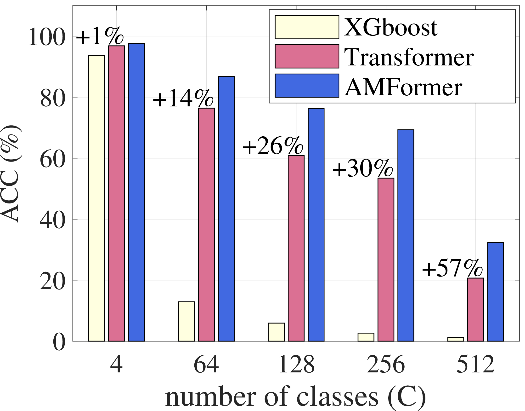
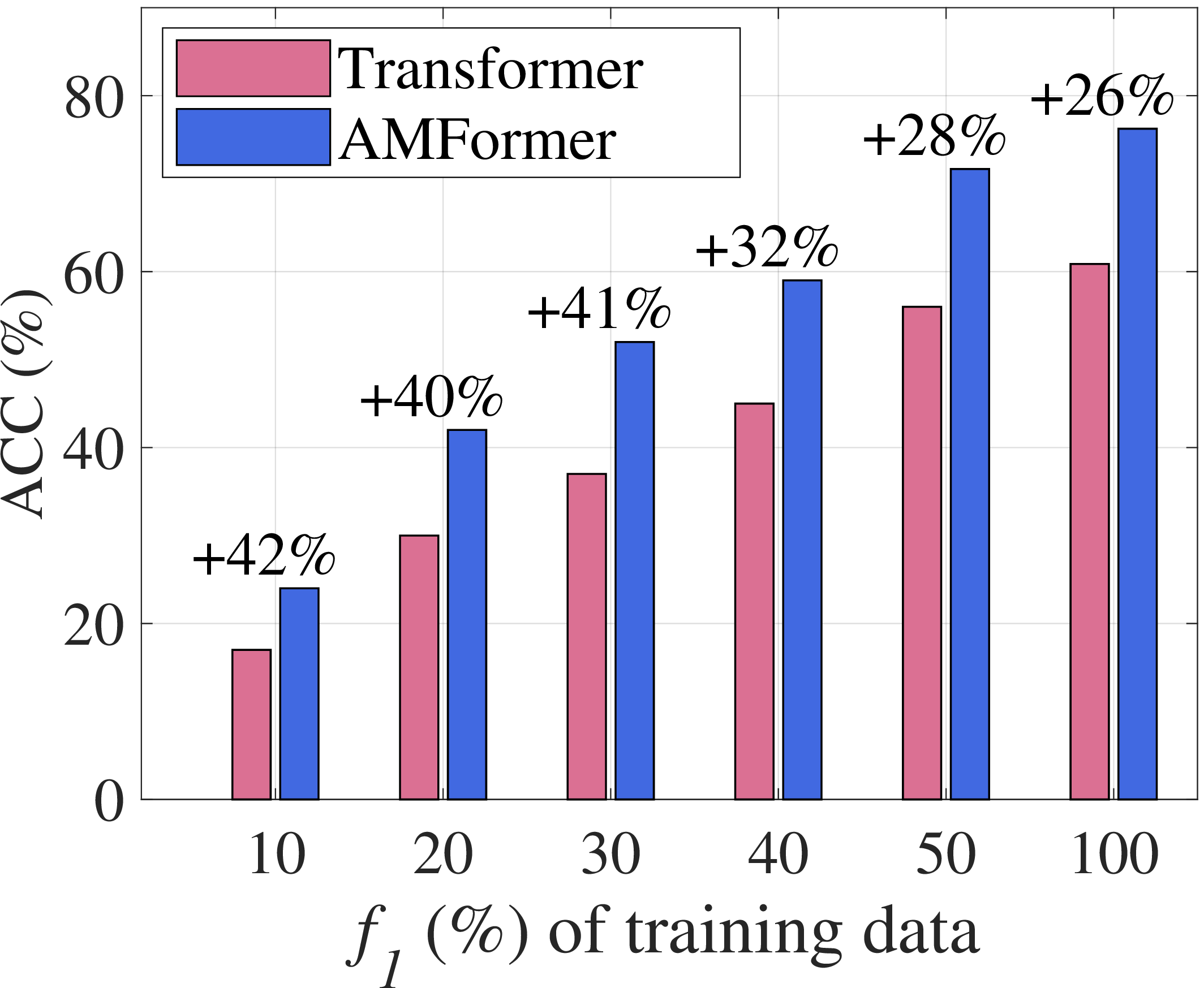

Figure 1: Results on synthetic data. The \(+x\%\) in the figure are the relative improvement of AMFormer over Transformer.. a — Fine-grained tabular data modeling, b — Data efficiency in training, c — Generalization
2 Related Work↩︎
In this section, we review related machine-learning methods for tabular data analysis and briefly introduce the ideas of local attention that inspire our prompt-based optimization.
Traditional methods. Tabular data could be naturally viewed as multi-dimensional vectors. Therefore, many classic machine-learning methods are applicable for mining tabular data, e.g., logistic regression, decision trees, and support vector machines [29]. Since features in tabular data are of varying importance typically, generalized additive models (GAM) [30], [31] remain popular for tabular data analysis. These models are more accurate than simple linear models with the introduction of shape functions and could produce the importance of individual features as model interpretation. Pairwise interactions have also been incorporated in GAMs for better model fitness [32]. Finally, gradient-boosted tree ensemble models, such as XGBoost [6], LightGBM [7], and CatBoost [8], are usually among the most effective in this category and have been widely deployed in real-life systems.
Deep learning models. As mentioned earlier, deep learning has been explored for dealing with tabular data recently, and the attempts could be classified into four classes. (C1) In Wide&Deep [10] and deep factorization machines [11], [12], multi-layer perceptrons (MLPs) are stacked aside the traditional shallow components to capture high-order feature interaction. (C2) NAM [14], NBM [15], and SIAN [16] combine GAMs with deep learning to enhance model expressive while still retraining interpretation. (C3) Alternatively, NODE [18] and Net-DNF [19] emulate key elements of tree models using neural networks, e.g., differentiable oblivious decision trees, and disjunctive normal forms with soft neural AND/OR gates. These tree-like models could then enjoy the merits of deep learning. (C4) Finally, relying on the global crossing capability, the transformer architecture has also been adapted to deep tabular learning. Typical models include FT-Transformer [21], AutoInt [20], and DCAP [33], where the attention mechanism is utilized for additive feature interaction.
Despite the above efforts, it still remains open for effective inductive bias of deep tabular learning. In this paper, we also consider transformer architecture as a promising candidate and further argue for the essential role of arithmetic feature interaction for deep tabular learning. Our proposed AMFormer enhances the classic transformer with such interaction through the parallel additive and multiplication attention operators and the interaction fusion layer. This is among the first in the literature and AMFormer has demonstrated consistently better performance compared to other transformer-based methods.
Local attention. The square nature of transformer would make it less efficient for a large context, which is the case for tabular data consisting of a large number of features. In this situation, an efficient transformer is required. Since words and pixels inherently possess continuity, it is natural to use local attention techniques to optimize efficiency. For instance, PVT [34] utilizes convolutional layers after each attention block to gather local information and gradually condenses the features. LongFormer [35] applies a moving window and calculates attention weights within the window. Sparse attention [36] introduces sparse factorizations of the full attention matrix. Different from the above, in this paper, we borrow the notion of prompts to localize the receptive field of features, and the number of prompts is independent of the number of features.
3 Empirical Evaluation on Synthetic Data↩︎
Recall that due to feature heterogeneity, the raw feature space of tabular data might not necessarily contain all determining features. Accordingly, we argue that arithmetic feature interaction is essential for deep tabular learning, aiming at supplementing these missing features with arithmetic as the prior knowledge in a reserved stage. To validate our hypothesis, we create a synthetic dataset inspired by the assumption of a generalized additive model with multi-order while sparse feature interaction [16].
Data construction. Our constructed dataset consists of eight features and the responses \(r\) are formulated as an additive mixture of arithmetic feature combinations: \[r = \sum_{i=1}^{K} \alpha_i \cdot \prod_{j=1}^8 x_{j}^{\beta_{ij}}.\] We fix the number \(K\) of additive terms to be much less than the number of possible feature combinations (e.g.,\(K=5\) in this work) and sample \(\alpha_i\) from a uniform distribution \(U(-1,1)\). Each exponent \(\beta_{ij}\) is uniformly sampled from \(\{1, 2, 3, 4\}\) with a 50% chance and is set to 0 otherwise. Thus, the expected number of involved features in each term is 4. After selecting all \(\alpha\) and \(\beta\) values, we randomly generate 200K instances of \((x_1, \dots, x_8, r)\) by sampling \(x_j\) from a log uniform distribution between 0.5 and 2. The above setups ensure that our synthetic data remains deterministic and sparse in terms of feature interaction, adhering to a mild assumption for feature interaction. Finally, all instances are divided into \(C\) equally-sized classes according to the response values \(r\), and we further split the data into 80%-20% for training and testing, respectively.
Results. To demonstrate the necessity of arithmetic feature interaction, we compare our AMFormer(we leave its technical details in the next section) with XGBoost and the classic transformer on the constructed data. We first evaluate the ability of fine-grained tabular data modeling of these approaches by varying the number \(C\) of classes from 4 to 512 and computing the test classification accuracy (Acc). The results are reported in Fig. 1 (a). When varying \(C\), the Acc of all approaches decreases with the increment of \(C\). The performance of XGBoost soon drops to a low level with \(C=64\). This is because XGBoost utilizes raw feature values \(x_j\) only, which could not handle the interaction between features and the response. Comparatively, both Transformer and AMFormer maintain relatively high Acc with larger \(C\), owing to the automatic feature engineering capacity of neural networks. We also find that AMFormer is consistently better than Transformer, with larger improvement for higher \(C\). This indicates the essential role of arithmetic feature interaction for fine-grained tabular data modeling.
In addition, through learning meaningful interaction patterns, we also expect AMFormer to have better training data efficiency and generalization to minority classes. To verify data efficiency, we fix \(C=128\), vary the fraction \(f_1\) of training data from 10% to 50%, and compute the test Acc of Transformer and AMFormer, reported in Fig. 1 (b). We omit XGBoost due to its uncompetitive performance. When varying \(f_1\), the Acc of both approaches increases with the increment of \(f_1\) as expected. Moreover, we observe consistently better relative improvement with less fraction of training data, e.g.,+40% with \(f_1 \le 30\%\) vs. the baseline +26%. Indeed, AMFormer trained with 40% data is almost on par with Transformer on all data.
To verify generalization, we also fix \(C=128\), manually turn half of the classes to minority classes by only reserving a fraction \(f_2\) of training data, and compute the test Acc of Transformer and AMFormer on minority classes, reported in Fig. 1 (c). Note that training data on rest classes and test data remain unfiltered. Similarly, we observe consistently better performance, in both absolute Acc or relative improvement, by AMFormer for minority classes.
From the above empirical evaluation, we believe that explicitly integrating arithmetic feature interaction is necessary for deep tabular learning.
4 Methodology↩︎
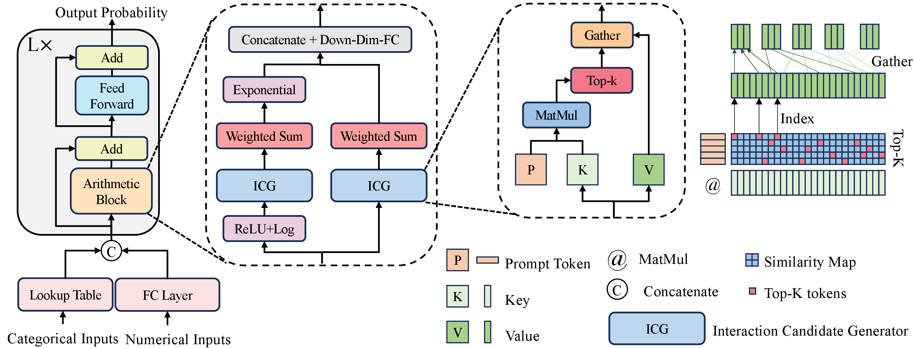
We now present the technical details of our AMFormer. The framework overview is given in Fig. 2, which closely resembles the classic Transformer architecture except for the Arithmetic Block. With \(d\) denoting the dimensionality of hidden states, AMFormer initiates the process by transforming raw features into representative embeddings, i.e., applying a 1-in-\(d\)-out linear layer for numerical features and a \(d\)-dimensional embedding lookup table for categorical features. Subsequently, these initial embeddings are processed through \(L\) sequential layers, which serve to augment them with vital context and interactive elements. Within each of these layers, an arithmetic block that executes parallel additive and multiplicative attention is adopted to deliberately foster arithmetic feature interactions. Residual connections and feed-forward networks are reserved to facilitate the flow of gradients and augment feature representation. Finally, AMFormer employs either a classification or a regression head to generate the final output based on these enriched embeddings. The key components in the arithmetic block include parallel attention and prompt tokens, which we will further discuss in the following.
4.1 Parallel Attention↩︎
The parallel attention is responsible for facilitating arithmetic feature interaction in AMFormer. The fundamental concept involves harnessing two parallel attention streams, each dedicated to computing either additive or multiplicative interaction candidates based on input feature embeddings. These computed candidates are subsequently concatenated and undergo further integration through a fully-connected (FC) layer. Consequently, the outputs of the FC layer can represent diverse combinations of input features achieved through arithmetic operations.
Formally, let \(N\) denote the number of input features in a specific layer \(l \in \{1, \dots, L\}\) and \(X \in \mathbb{R}^{N \times d}\) the corresponding feature embedding matrix. As the layers in AMFormer are structurally identical, differing only in their parameters, we forego mentioning the layer index for ease of notation. Recall that the classic attention [37] is inherently additive. We therefore derive log-scaled embeddings in the multiplicative stream [38]: \[X_{log} = {\rm log}({\rm ReLU}(X)+\epsilon), \label{eq:log}\tag{1}\] where \(\epsilon\) prevents \(\log 0\). Classic attention in the log space, combined with an exponential operator, is then capable of learning multiplicative interaction.
We next elaborate on the shared attention part of the two streams, which aims to prepare useful additive and multiplicative feature interaction for the prediction task. Taking the additive stream for instance, we first generate the query \(Q=XW^Q\), key \(K=XW^K\), and value \(V=XW^V\) embeddings with input embeddings \(X\) and trainable parameters \(W^{Q/K/V} \in \mathbb{R}^{d \times d}\). The product \(QK^T\) gives the affinity between input features and could be understood as the likelihood of yielding meaningful interaction in our case. The output by the additive stream, calculated as the weighted sum of value embeddings according to the normalized product: \[O^A = {\rm softmax}(\frac{QK^T}{\sqrt{d}})V \in \mathbb{R}^{N \times d}, \label{eq:attention}\tag{2}\] enriches each input feature with vital interactive information from other features and, hence, could be regarded as additive interaction candidates.
The above soft attention establishes a connection between every pair of features, while the interaction on tabular data is mostly sparse [14], [15]. Inspired, we further revise Eq. (2 ) into hard attention. That is, we retrieve and retain the top-\(k\) highest entries in each row of \(QK^T\) while masking other entries with a large negative constant, i.e., becoming 0 after softmax. As such, each feature could only interact with \(k\) features and it suffices to choose a small integer for hyperparameter \(k\), being independent with the number \(N\) of input features, to ensure sparse interaction.
Similarly, we could obtain the multiplicative stream output \(O^M \in \mathbb{R}^{N \times d}\) by using the log-scaled \(X_{log}\), another set of trainable parameters, and an additional exponential operator. The central idea of our AMFormer is to provide complete arithmetic ability in every single layer. To achieve the goal, we further concatenate the two outputs \(O^A\) and \(O^M\) and apply an FC layer along the candidate dimension: \[O = {\rm FC}({\rm VConcat}([O^A, O^M])^T)^T. \label{eq:combine}\tag{3}\] Note that \({\rm VConcat}([O^A, O^M])\) performs vertical concatenation, resulting in a shape of \({2N \times d}\), \({\rm FC}\) is a fully-connected layer that also decreases the number of dimension from \(2N\) to \(N\), and the two transposition operators assure the fusion of interaction candidates. To summarize, the parallel attention in the arithmetic block first extracts additive and multiplicative interaction candidates independently, and the candidates are subsequently mixed to facilitate complete arithmetic feature interaction in a single layer of AMFormer.
4.2 Optimization with Prompt Tokens↩︎
The architecture described by far potentially faces a couple of practical challenges. Initially, the self-attention mechanism has a complexity that grows quadratically with the number of features, specifically \(O(N^2d)\), resulting in inefficiencies in time and memory for large feature sets [39], [40]. Additionally, tabular datasets often exhibit interaction patterns that are data-invariant, e.g., those relating to domain patterns, while the current purely data-reliant architecture has trouble capturing them. To tackle the two issues, we have incorporated an optimization strategy that utilizes prompt tokens within AMFormer.
The main idea is to substitute the data-dependent query matrix \(Q\) with a set of trainable prompt token embeddings, represented as a parameter matrix \(P \in \mathbb{R}^{N_p \times d}\). Each of these prompt tokens is designed to facilitate the creation of valuable additive or multiplicative interactions among features, considering up to \(k\) features at a time. The quantity \(N_p\) of prompt tokens could be much less than the overall number of features on large datasets. Consequently, the time and memory complexities associated with AMFormer become linear relative to the number \(N\) of input features, thus enhancing the model’s capability to handle extensive datasets. Additionally, this approach enables AMFormer to inherently learn and establish patterns of feature interaction that are consistent across different samples. The strategic use of prompt tokens in conjunction with the top-k selection also allows AMFormer to disregard immaterial correlations in the data. This not only helps in preventing overfitting but also improves the model’s resilience against data noise [41], [42].
In practice, we recommend fixing \(N_p=N\) for datasets with a few hundred features. In cases of larger datasets, it is suggested to start with \(N_p\) at 256 or 512 and then reduce this number by half for each ensuing layer.
5 Experiments↩︎
| Dataset | Task type | Metric | # Train | # Valid | # Test | # Num. features | # Cate. features |
|---|---|---|---|---|---|---|---|
| EP | binary classification | Acc | 320,000 | 80,000 | 100,000 | 2,000 | / |
| HC | binary classification | AUC | 200,496 | 45,512 | 61,503 | 104 | 16 |
| CO | multi-classification | Acc | 371,847 | 92,962 | 116,203 | 54 | / |
| MI | regression | MSE | 72,3412 | 235,259 | 24,1521 | 136 | / |
| Dataset | XGBoost | NODE | DCN-V2 | DCAP | AutoInt | FT-Trans. | ||
|---|---|---|---|---|---|---|---|---|
| EP \(\uparrow\) | 87.32 (8) | 89.60 (3) | 88.22 (7) | 89.24 (4) | 88.48 (6) | 89.05 (5) | 89.71 (2) | 89.83 (1) |
| HC \(\uparrow\) | 74.59 (7) | 74.93 (6) | 72.34 (8) | 75.63 (2) | 75.01 (5) | 75.07 (4) | 75.57 (3) | 75.67 (1) |
| CO \(\uparrow\) | 96.72 (3) | 92.31 (7) | 90.78 (8) | 96.21 (5) | 92.40 (6) | 96.60 (4) | 97.36 (1) | 97.26 (2) |
| MI \(\downarrow\) | 0.5642 (3) | 0.5644 (4) | 0.6043 (8) | 0.5753 (6) | 0.5864 (7) | 0.5717 (5) | 0.5606 (2) | 0.5557 (1) |
| Rank \(\pm\) std | \(5.3\pm2.6\) | \(5.0\pm1.8\) | \(7.8\pm0.5\) | \(4.3\pm1.7\) | \(6.0\pm0.8\) | \(4.5\pm0.6\) | \(2.0\pm0.8\) |
In this section, we further evaluate our AMFormer in real-world scenarios. Using four datasets, we conduct extensive experiments to evaluate: (i) the overall effectiveness of AMFormer compared with other competitive methods, (ii) the rationale of each building component in AMFormer, (iii) the impacts of the prompt-based optimization in effectiveness and scalability, and (iv) the sensitivity to key parameters.
5.1 Experimental Setup↩︎
Datasets. We choose four real-world datasets for evaluation.
EP (Epsilon) is a simulated physics dataset from [43], which uses 2,000 normalized numerical features for binary classification.
HC (Home Credit Default Risk) uses both numerical and categorical features to predict clients’ binary repayment abilities, with a ratio of around 1:10 for positive to negative samples [44].
CO (Covtype) is a multi-classification dataset that utilizes surrounding characteristics to predict types of trees growing in an area [45].
MI (MSLR-WEB10K) is a learn-to-rank dataset for query-URL relevance ranking [46]. It contains 136 numerical features and relevance scores are drawn from \(\{0,1,2,3,4\}\).
We adopt the same learning tasks, i.e., binary/multi-classification and regression, and metrics, i.e., accuracy (Acc), area under the ROC curve (AUC), and mean square error (MSE), as previous studies. Table 1 summarizes the statistics and evaluation settings of these datasets. We normalize the numerical features to have zero mean and unit variance before feeding into models.
Baselines. We compare AMFormer to a variety of baseline methods, including the competitive tree ensemble method XGBoost [6], differentiable tree model NODE [18], transformer-based approaches AutoInt [20] and FT-Transformer [21], and the recent deep cross nets DCN-V2 [47] and DCAP [33]. Our AMFormer is a general deep tabular learning module and we plug it into FT-Transformer and AutoInt, leading to two variants AMF-A and AMF-F for comparison, respectively.
Implementation. All tested models are implemented with PyTorch v1.12 [48]. We use the recommended model parameters in the original papers for baseline methods and those of XGBoost follow [21]. Notably, AutoInt and FT-Transformer use a dimensionality of 32 and 192 for embeddings, respectively, which are inherited in AMF-A and AMF-F. We adopt Adam with betas=(0.9, 0.999) and eps=1e-8 for optimization. The learning rate first linearly increases to 1e-3 in the first 1k steps and then decays by 90% every 20k steps by default, except for the HC data with an initial 1e-4 and 4k decaying steps. The default batch size is 512, which reduces to 32 for transformer-based methods on the EP data due to GPU-memory limitation. We report the detailed hyper-parameters of all methods in the supplement. All tests are conducted on a machine with 104 Intel(R) Xeon(R) Platinum 8269CY CPUs and an NVIDIA Tesla A100-SXM-40GB.
We next present our findings.
5.2 Comparison with Known Methods↩︎
In the first set of tests, we evaluate the overall effectiveness of our approach by comparing its variants with the considered baselines. The metrics on the test set are presented in Table 2 and we conclude the following.
First, DCN-V2 performs the worst compared with other tested approaches. Note that it utilizes MLP to capture high-order feature interaction, which turns out to be less effective for tabular data. AutoInt only preserves the multi-head self-attention while dropping the feed-forward net and residual connection from its transformer architecture, and its effectiveness remains not competitive either. Inspired, we keep these operators in our AMFormer.
For the rest baselines, we observe inconsistent performance across different datasets. The top-performing methods are diverse, e.g., XGBoost on CO and MI, NODE on EP, and DCAP on HC. This result has somehow demonstrated the challenge of identifying a unified modeling bias for tabular data analysis. Overall, we find that DCAP and FT-Transformer are the best among these baselines according to the average performance rank on all datasets. Both approaches are based on the transformer architecture, indicating its potential for deep tabular learning. However, it is worth noting that none of the deep models could outperform XGBoost on all datasets.
Finally, the two variants of AMFormer are consistently better than the six tested baselines on the four datasets, except for AMF-A on the HC data where it slightly underperforms compared to DCAP. This implies that AMFormer consistently enhances the performance of the two backbone models on all datasets. Specifically, in classification tasks, AMFormer improves the accuracy or AUC of AutoInt and FT-transformer by at least 0.5%, with improvements of up to 1.23% and 4.96% observed on the EP and CO data for AutoInt. In regression tasks, the MSE of the two backbone models decreases by more than 0.016. The effectiveness and stability of AMFormer result in significantly better performance rankings for AMF-A and AMF-F compared to all existing approaches, marking a significant milestone for deep learning on tabular data. From our perspective, we believe that AMFormer effectively addresses the question of whether deep learning is necessary for tabular data.
5.3 Ablation Study↩︎
| Backbone | Add. | Multi. | Prompt | EP \(\uparrow\) | MI \(\downarrow\) |
|---|---|---|---|---|---|
| AutoInt | ✔ | - | - | 88.48 | 0.5864 |
| ✔ | - | ✔ | 89.61 | 0.5638 | |
| - | ✔ | - | 89.53 | 0.5748 | |
| - | ✔ | ✔ | 89.65 | 0.5631 | |
| ✔ | ✔ | - | 89.55 | 0.5639 | |
| ✔ | ✔ | ✔ | 89.71 | 0.5606 | |
| FT-Trans. | ✔ | - | - | 89.05 | 0.5717 |
| ✔ | - | ✔ | 89.80 | 0.5633 | |
| - | ✔ | - | 50.05 | 0.5624 | |
| - | ✔ | ✔ | 50.05 | 0.5605 | |
| ✔ | ✔ | - | 89.58 | 0.5585 | |
| ✔ | ✔ | ✔ | 89.83 | 0.5557 |
We next conduct an ablation study to evaluate the impacts of the building component within our AMFormer, i.e., the additive attention, the multiplicative attention, and the prompt-based optimization. Similarly, we consider two backbone models and evaluate the test metrics by using different combinations of the components on the EP and MI datasets. Note that EP has the largest number of features and MI is the only regression dataset. The results are reported in Table 3 and we find the following.
First, we find that multiplicative interaction is important, and using multiplicative attention alone could obtain better results than using classic additive attention alone in three of the four testing cases (row 1 vs. row 3), except for using FT-Transformer as the base model on EP. Moreover, using parallel additive and multiplicative attention consistently improves the effectiveness in all scenarios (row 5 vs. 1&3), indicating the usefulness of arithmetic feature interaction for tabular data analysis. In addition, our prompt-based optimization also leads to consistent performance improvement (rows 1&3&5 vs. 2&4&6, respectively). This is because prompts could stabilize the interaction patterns which do not vary with examples and this is very important for tabular data. Moreover, when dealing with a large number of features, a small number of prompts could reduce irrelevant interactions in redundant features.
| Method | Prompt | Train (hr) | GFLOPS | GPU-M |
|---|---|---|---|---|
| AutoInt | - | 16.81 | 7.2 | 33 GB |
| FT-Trans | - | 19.64 | 9.7 | 34 GB |
| - | 25.77 | 12.3 | 36 GB | |
| - | 20.88 | 11.3 | 38 GB | |
| ✔ | 2.93 | 1.3 | 17 GB | |
| ✔ | 3.11 | 0.7 | 18 GB | |
| % | ✔ | 11.37% | 10.45% | 51.51% |
| % | ✔ | 14.89% | 6.16% | 52.94% |
The complexity of attention has always been a very efficiency-critical part. With an \(\mathcal{O}(N^{2})\) complexity to the number \(N\) of tokens/features, the computational cost will increase quadratically with the increase of token number, and the attention map will also occupy a lot of GPU memory during training. From Table 4 we find that the overall training time for FT-Transformer and AutoInt exceeds 15 hours. For our AMFormer without prompts, the training time even exceeds 20 hours. Our AMFormer incorporates the additional multiplicative attention, which requires more FLOPs and results in longer training time. After applying the prompt optimization to limit feature interaction, our AMFormer reduces computational resource by approximately 90% and 94% and achieves approximately 7 times faster training speed, i.e., only around 3 hours of training time. Moreover, with the same batchsize, our AMFormer needs only 17 GB GPU-memory while its counterparts take up at least 33 GB GPU-memory. Less memory usage makes it possible to train and employ our AMFormer on less-powerful devices.
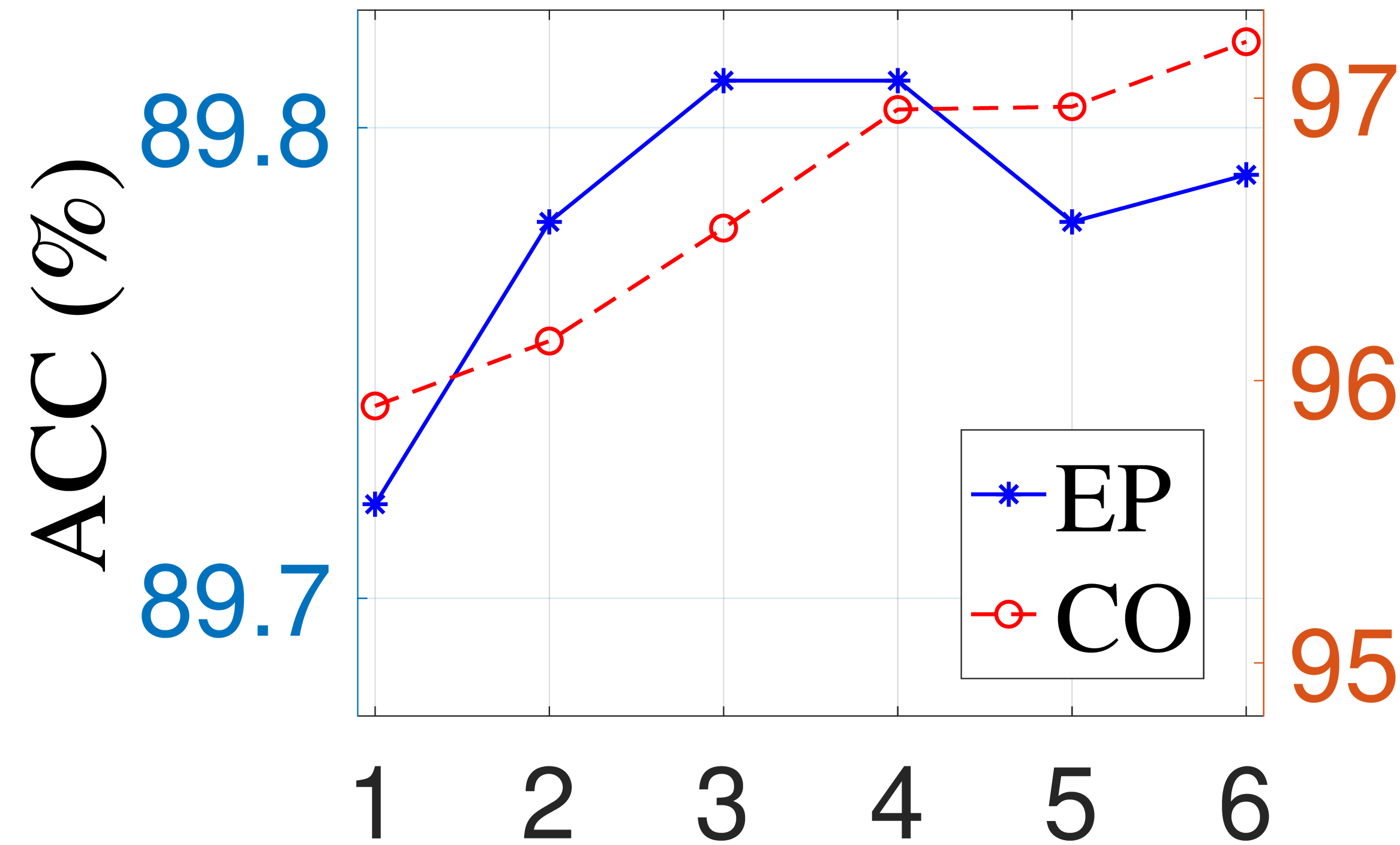
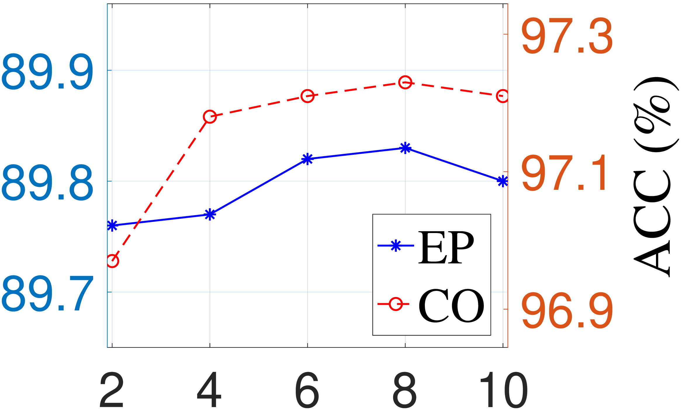
Figure 3: Impacts of layer number \(L\) and parameter \(k\).. a — Layer number \(L\), b — Parameter \(k\)
| \(N_P\) | 32 | 64 | 128 | 256 | 512 | 1024 |
| EP | 89.75 | 89.79 | 89.77 | 89.81 | 89.83 | 89.76 |
5.4 Parameter Sensitivity↩︎
Finally, we evaluate the parameter sensitivity of AMFormer. To examine the impact of \(L\), we vary \(L\) from 1 to 6, fix the other parameters to their default values, and test the Acc results on the EP and CO dataset, as shown in Fig. 3 (a). When increasing \(L\), the Acc first increases and then decreases on EP while it continues increasing on CO. The best Acc is attained at \(L=3\) for EP and \(L=6\) for CO. Note that the accuracy metric on the CO dataset starts to plateau at \(L=4\). Overall, we believe that approximately \(3\sim4\) layers are sufficient for feature extraction.
When dealing with large datasets, we set the number of prompt tokens as \(N_P\) in the first layer, and then reduce this number by half for each subsequent layer. As shown in Table 5, on the large EP data, a small \(N_P\) (\(<256\)) results in slightly worse performance caused by insufficient learning, while the performance tends to saturate around 256. However, increasing \(N_P\) further leads to a decrease in performance, because large \(N_P\) tends to cause redundancy and overfitting. Although 512 tokens exhibit better performance than 256, the trade-off between performance and efficiency makes 256 a balanced choice.
We further present the sensitivity results of parameter \(k\), i.e., top-k, for forming feature interaction. The results on EP and CO are shown in Fig. 3 (b), from which we find that the Acc increases first from 2 to 8 and then decreases slightly. Overall, large \(k\) is more suitable for AMFormer. This is because the impacts of less relevant features are decreased by the affinity weights. However, there is a risk of overfitting in practical training and larger \(k\) can then have a negative impact. We thus recommend \(k=8\) by default.
6 Conclusion↩︎
This paper studied the effective inductive bias of deep models on tabular data. We hypothesized that arithmetic feature interaction is necessary for tabular deep learning and integrated this idea in the transformer architecture to derive AMFormer. We verified the effectiveness of AMFormer on both synthetic and real-world data. The results of our synthetic data demonstrated its better capacity for fine-grained tabular data modeling, data efficiency in training, and generalization. Moreover, extensive experiments on real-world data further confirmed its consistent effectiveness, the rationale behind each building block, and the scalability to handle large-scale data. We thus believe that AMFormer has established a strong inductive bias for deep tabular learning.
Acknowledgments↩︎
This research was partially supported by National Natural Science Foundation of China under grants No. 62106218 and No. 62132017, Zhejiang Key R&D Program of China under grant No. 2023C03053.
Appendix A: Extra Results on Parameter Sensitivity↩︎
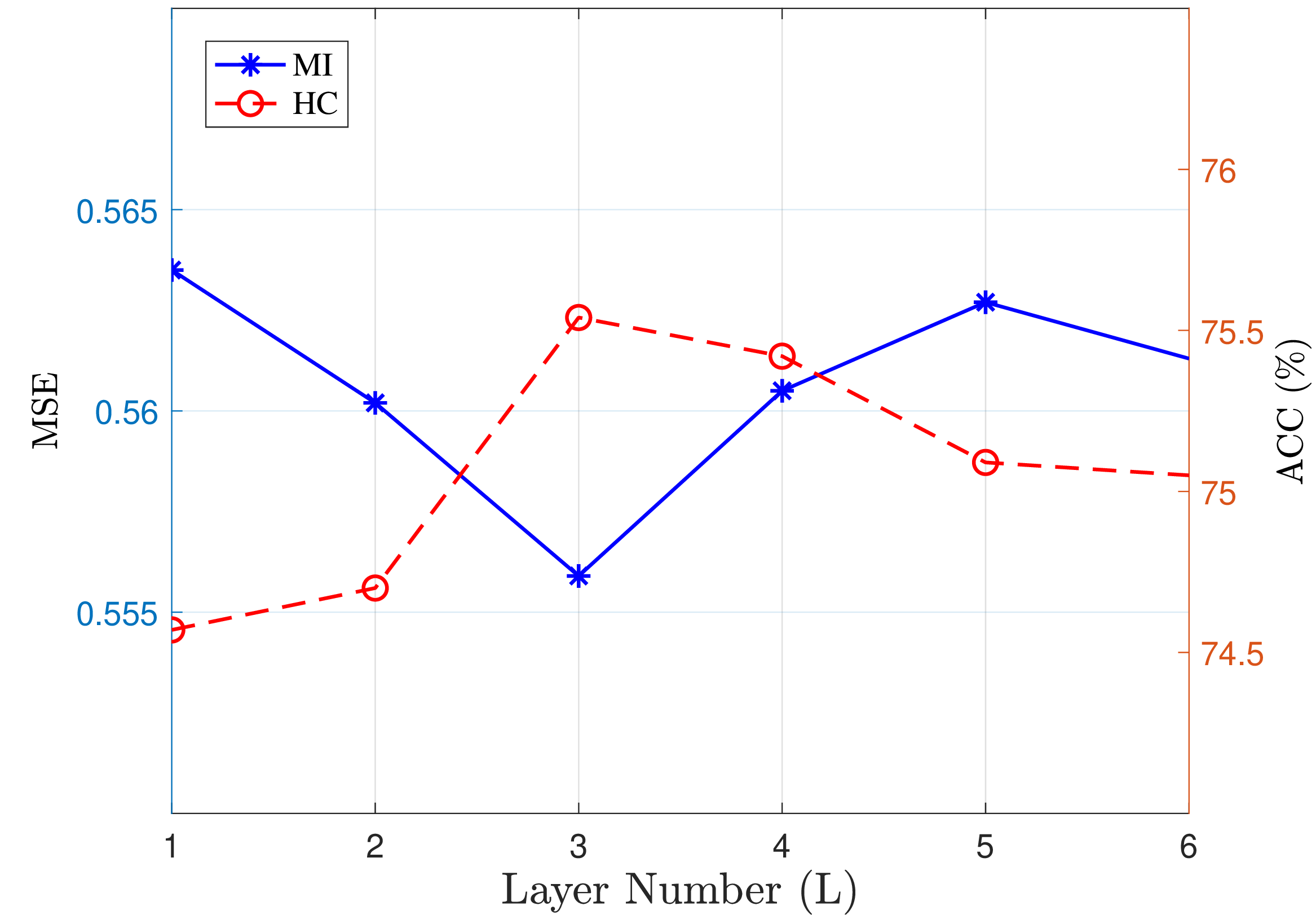
We also investigate the effect of the parameter \(L\) on the MI and HC datasets, while keeping the default settings for other parameters. The MSE (\(\downarrow\)) and ACC (\(\uparrow\)) results are illustrated in Fig. 4. Similar to the performance on the EP and CO datasets, as the number of layers increases, the overall performance of our AMFormer initially improves and then starts to decline. The optimal performance is achieved on both datasets when \(L=3\).
Considering the results obtained from all four datasets, it can be concluded that \(L=3\) is a parameter that universally applies across different datasets.
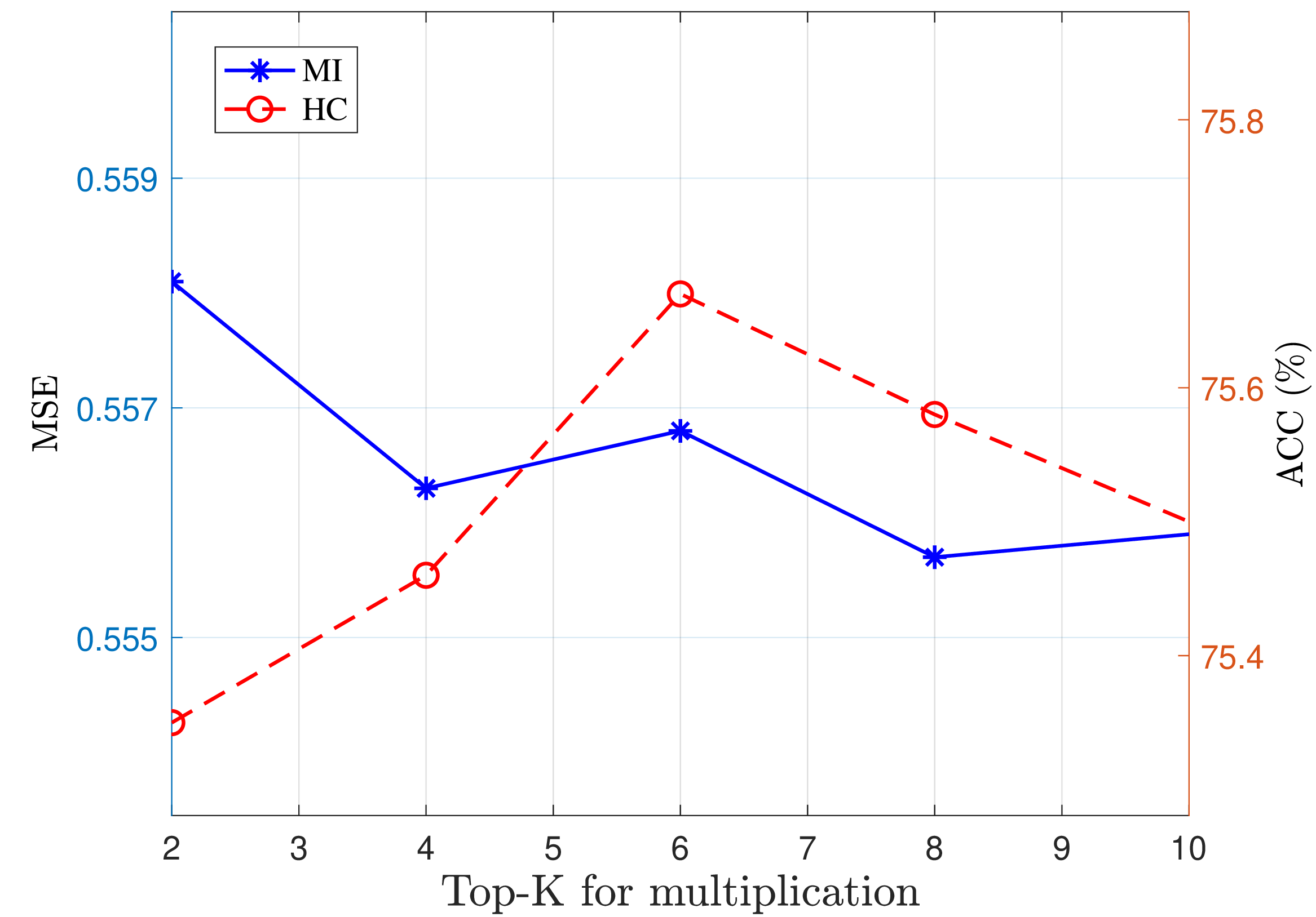
With the optimal number of layers \(L\), we further explore the impact of different values of \(K\) on these two datasets. As depicted in Fig. 5, the ACC on the HC dataset demonstrates a rapid increase before \(K=6\) followed by a slight decline, while the MSE on the MI dataset continues to decrease and stabilizes after \(K=8\). These findings suggest that a larger value of \(K\) can enhance the performance of our AMFormer, but increasing \(K\) beyond a certain threshold may lead to a slight decline in performance.
| dimension | 1024 |
| # Layer | 2 |
| choice-function | entmax15 |
| bin-function | entmoid15 |
| # Layers | 3 |
| dimension | 32 for AutoInt, 192 otherwise |
| heads | 8 |
| FF-dropout | 0.1 |
| Attention-dropout | 0.2 |
| layer-num | 2 |
| embedding-size | 16 |
| dnn-hidden-units | (562, 562, 562) |
| init-std | 0.0001 |
| l2-reg | 0.00001 |
| drop-rate | 0.5 |
| booster | "gbtree" |
| early-stopping-rounds | 50 |
| n-estimators | 2000 |
Appendix B: Default Settings for Each Method↩︎
In this section, we provide the implementation details for all models. We utilize the official implementation for NODE 3, which uses the default hyper-parameter settings presented in Table 6. As shown Table 7, Transformer-based methods share most of the hyper-parameters, except for the feature dimension. AutoInt uses a feature dimension of 32, while FT-Transformer and DCAP use a feature dimension of 192. The hyper-parameters for DCN-V2 are listed in Table 8.It should be noted that the embedding feature within DCN-V2 is calculated as the sum of the number of numerical features and the product of the number of categorical features and the embedding size. Additionally, the default hyperparameter settings for XGBoost can be found in Table 9.