Joint channel estimation and data detection in massive MIMO systems based on diffusion models
November 17, 2023
Abstract
We propose a joint channel estimation and data detection algorithm for massive multilple-input multiple-output systems based on diffusion models. Our proposed method solves the blind inverse problem by sampling from the joint posterior distribution of the symbols and channels and computing an approximate maximum a posteriori estimation. To achieve this, we construct a diffusion process that models the joint distribution of the channels and symbols given noisy observations, and then run the reverse process to generate the samples. A unique contribution of the algorithm is to include the discrete prior distribution of the symbols and a learned prior for the channels. Indeed, this is key as it allows a more efficient exploration of the joint search space and, therefore, enhances the sampling process. Through numerical experiments, we demonstrate that our method yields a lower normalized mean squared error than competing approaches and reduces the pilot overhead.
Joint channel estimation and data detection, score-based generative models, Langevin diffusion, blind inverse problems.
1 Introduction↩︎
Massive multiple-input multiple-output (MIMO) systems are pivotal for advancing wireless communication [1]. These systems feature a large number of antennas at base stations, enabling simultaneous support for multiple users. While crucial for the transition to 6G cellular networks [2], MIMO systems pose challenges, such as achieving low-complexity detection and precise channel estimation. This paper focuses on these physical layer issues.
Exact MIMO detection is NP-hard [3]. With \(N_u\) users and \(\kappa\)-symbol modulation, the maximum likelihood estimator’s decoding complexity is exponential \(\mathcal{O}(\kappa^{N_u})\), rendering it infeasible for sizable systems. Additionally, it relies on perfect channel state information (CSI), usually unavailable. Hence, an efficient channel estimation method is crucial, but it is challenging in massive MIMO due to the high dimensionality of the system and the constraint on the number of pilot signals [4]. As a consequence, a joint optimization approach (still NP-hard) to estimate both the data and the channel is necessary to tackle these issues in high-dimensional systems [5], [6]. Different approximate solutions based on gradient descent have been proposed for single-input multiple-output systems [7]. Recently, new methods have been proposed for massive MIMO. In [8], the authors proposed an algorithm that iteratively solves a relaxed version of the maximum a posteriori joint channel estimation and data detection (MAP-JED) problem that exploits the sparsity of the channel, while in [9] a solution based on deep neural networks, and more specifically, algorithmic unfolding, was proposed. In this work, we introduce a novel approach based on diffusion models, also known as score-based generative modeling.
Diffusion models, known for their versatility, have excelled across diverse applications [10]. These models transform training data into white Gaussian noise (the forward process) and then run the reverse transformation (the generative process) to generate new data. Leveraging their ability to generate high-dimensional data from unknown probability distributions, diffusion models have achieved state-of-the-art results in various areas, such as denoising and inpainting in image processing [11], [12]. In wireless technology, they have been used to derive a massive MIMO detector based on Langevin diffusion [13], [14], and for channel estimation [15], both of which have shown remarkable results. However, these methods are tailored for problems with known forward operators and may not apply to blind inverse problems, where the operator is unknown. Recent advances in image processing aim to address these challenges [16], [17], to provide more comprehensive solutions.
In this work, inspired by the above results, we propose a framework to solve the joint massive MIMO channel estimation and data detection problem based on score-based generative modeling. To achieve this, we construct a diffusion process that models the joint distribution of the channels and symbols given noisy observations and then sample it by running the reverse diffusion. Our proposed method allows us to incorporate prior information on each variable to enhance the sampling process.
Contribution. The contributions of this paper are twofold:
1) We propose an algorithm for solving the joint massive MIMO detection and channel estimation problem based on diffusion models, which allows us to incorporate both the discrete prior of the symbols and a learned prior for the channel.
2) Through numerical experiments, we analyze the behavior of our method for different hyperparameter settings and demonstrate the performance gain of our joint solution compared to separate channel estimation and data detection.
2 System model and problem formulation↩︎
We focus on the uplink of a massive MIMO communication system. We consider \(N_u\) single-antenna transmitters or UEs that transmit pilots and data to a receiving base station equipped with \(N_r\) antennas, under a block-fading scenario with a coherence time of \(K = P + D\) time slots; \(P\) time slots are reserved for pilots and \(D\) time slots are used for payload data. Under this scenario, the forward model for the MIMO system is defined as \[\label{E:mimo95model} \bbY = \bbH \bbX + \bbZ,\tag{1}\] where \(\bbH \in \mathbb{C}^{N_r \times N_u}\) is the channel matrix, each \(\{[\bbZ]_{:j}\}_{j=1}^K \sim \mathcal{CN}(\bb0, \sigma_0^2\bbI_{N_r})\) is a vector of complex circular Gaussian noise, \(\bbX = [\bbX_P, \bbX_D] \in \mathcal{X}^{N_u \times K}\) is the vector of transmitted data, where \(\bbX_P\in \mathcal{X}^{N_u \times P}\) corresponds to the pilots while \(\bbX_D \in \mathcal{X}^{N_u \times D}\) is the data, and \(\mathcal{X}\) is a finite set of constellation points, and \(\bbY \in \mathbb{C}^{N_r \times K}\) is the received vector. We consider quadrature amplitude modulation (QAM) throughout this work with symbols normalized to attain unit average power. All the users transmit with the same modulation and each symbol has the same probability of being chosen by each of the \(N_{u}\) users. Moreover, we assume that \(\bbH\) is unknown while \(\sigma_0^2\) is known at the receiver. Under this configuration, the joint channel estimation and data detection problem can be stated as follows.
****Problem** 1. Given observations \(\bbY\) and pilots \(\bbX_{P}\) following 1 , find the MAP estimate of both \(\bbX_D\) and \(\bbH\).**
Given that \(\bbZ\) in 1 is a random variable, a natural way of solving Problem 1 is to search for \(\{\bbH, \bbX_D\}\) that maximizes its posterior probability given the noisy observations \(\bbY\) and pilots \(\bbX_P\). Hence, the Bayes’ optimal decision rule can be written as \[\begin{align} \label{eq:map} \{\hat{\bbH}_{\mathrm{MAP}}, \hat{\bbX}_{D_{\mathrm{MAP}}}\} &= \argmax_{\substack{\bbX_D \in \mathcal{X}^{N_u\times D}, \\ \bbH \in \mbC^{N_r\times N_u}}}\,\, p(\bbX_D, \bbH|\bbY,\bbX_P) \\ \nonumber&= \argmax_{\substack{\bbX_D \in \mathcal{X}^{N_u\times D}, \\ \bbH \in \mbC^{N_r\times N_u}}}\,\, p_{\bbZ}(\bbY - \bbH\bbX)p(\bbX)p(\bbH). \end{align}\tag{2}\] The problem in 2 is known as MAP-JED. Since we assume that the symbols’ prior distribution is uniform among the constellation elements and the measurement noise \(\bbZ\) is Gaussian, the MAP-JED formulation boils down to the following optimization problem \[\label{eq:ml} \{\hat{\bbH}_{\mathrm{MAP}}, \hat{\bbX}_{D_{\mathrm{MAP}}}\} = \argmin_{\substack{\bbX_D \in \mathcal{X}^{N_u \times D}, \\ \bbH \in \mbC^{N_r\times N_u}}}\,\, ||\bbY - \bbH\bbX||^2_2 - \log p(\bbH),\tag{3}\] This problem is NP-hard due to the discrete nature of the finite constellation constraint \(\bbX_D \in \mathcal{X}^{N_u}\) and the non-convexity of the product between decision variables. Thus, several schemes have been proposed in the last decades to provide efficient approximate solutions to Problem 1, as mentioned in Section 1. In this paper, we propose to solve Problem 1 by (approximately) sampling from the posterior distribution in 2 using an annealed Langevin dynamic.
3 Joint channel estimation and data detection based on Langevin dynamics↩︎
In Section 3.1, we briefly introduce the Langevin diffusion and score-based generative modeling. Then, in Section 3.2, we describe our algorithm for joint posterior sampling based on Langevin dynamics, and detail the expression of the score functions involved in the diffusion process.
3.1 Langevin diffusion and posterior sampling↩︎
In general, a diffusion process is a continuous-time Markov process on the variable \(\bbX \in \reals^d\) that solves the Ito equation \[\begin{align} \label{eq:diffusion} \text{d}\bbX_t &= \bbf(\bbX_t, t)\text{d}t + \bbg(t)\text{d}\bbW_t, \end{align}\tag{4}\] where \(\bbW\) is a standard \(d\)-dimensional Brownian motion, \(\bbf(\bbX_t,t)\) and \(\bbg(t)\) are the drift and diffusion term respectively, which are assumed to be Lipschitz continuous for all t. The Langevin diffusion is a particular type of diffusion process, which is obtained when \(f(\bbX_t, t) = \nabla_{\bbX_t}\log p(\bbX_t)\) and \(g(t) = \sqrt{2 \tau}\) [18]. Under mild conditions, it can be shown that the invariant distribution of the continuous-time process is \(\pi(\bbX) \propto p(\bbX)^{1/\tau}\) [18]. In particular, if \(\tau = 1\), then \(\pi(\bbX) \propto p(\bbX)\).
The Euler-Maruyama discretization of 4 gives rise to the unadjusted Langevin algorithm (ULA), which is an MCMC algorithm [19], described by the following discrete equation \[\label{eq:langevin} \bbX_{k+1} = \bbX_k + \epsilon \nabla_{\bbX_k}\log p(\bbX_k) + \sqrt{2\epsilon \tau}\, \bbZ_k,\tag{5}\] where \(\bbZ_k\sim\ccalN(\bb0, \bbI)\). In essence, ULA generates samples from a target distribution \(p(\bbX)\) by iteratively moving in the direction of the gradient of the logarithm of the target density, known as the score function, and introducing noise to avoid local maxima. Under some regularity conditions, the distribution of \(\bbX_k\) converges to \(p(\bbX)\) when \(\epsilon \rightarrow 0\) and \(k \rightarrow \infty\). Although this result is asymptotic, also non-asymptotic convergence results have been obtained under some conditions on the target distribution [20].
Score-based generative modeling. It should be noted that the only requirement for sampling from \(p(\bbX)\) using this procedure is knowing the score function, which is unknown in general. Hence, we consider denoising score matching [21] to estimate the score by training a neural network, known as a score network, that parameterizes the score. In a nutshell, the method is as follows: given a training dataset \(\{\bbX_i\}_{i=1}^n\) drawn from the distribution \(p(\bbX)\), we first perturb the data at different scales with Gaussian kernels of variance \(\{\sigma_l\}_{l=1}^L\) associated with each scale \(l\). This perturbation defines a distribution \(q_{\sigma_l}(\tilde{\bbX})\) where \(\tilde{\bbX}\) is the perturbed data. Finally, the authors in [22] propose to estimate a joint score network \(\bbs_{\theta}(\bbX, \sigma)\) via score matching, i.e., by minimizing the following loss \[\label{eq:loss} \ccalL(\bbtheta) \!\!=\!\! \frac{1}{2L}\sum_{l=1}^L \lambda(\sigma_l)\mathbb{E}_{p(\bbX)q_{\sigma_l}(\tilde{\bbX}|\bbX)}\bigg[\bigg|\bigg|\bbs_{\theta}(\tilde{\bbX}, \sigma_l) + \frac{\tilde{\bbX} - \bbX}{\sigma_l^2}\bigg|\bigg|^2_2\bigg].\tag{6}\] where \(\lambda(\sigma_l)\) is a pre-defined weight depending on \(\sigma_l\). After training, we can replace \(\nabla_{\bbX_k}\log p(\bbX_k)\) in 5 by \(\bbs_{\theta}(\bbX, \sigma)\) and generate samples from the target distribution \(p(\bbX)\). In Section 3.2, we leverage this and use a pre-trained score network for the channel distribution.
3.2 Joint diffusion posterior sampling↩︎
Recall our goal is to solve Problem 1 via ULA 5 by sampling from the joint posterior 2 . Hence, we must adapt the framework from Section 3.1 for several reasons. First, we are interested in sampling from the joint posterior \(p(\bbX_D, \bbH|\bbY, \bbX_P)\), not just \(p(\bbX)\). This necessitates computing the score of the joint posterior, specifically gradients with respect to \(\bbX_D\) and \(\bbH\), expressed as: \[\begin{align} \label{E:score95function} \nabla_{\bbX_D}\log p(\bbX_D, \bbH|\bbY, \bbX_P) &= \nabla_{\bbX_D}\log p(\bbY|\bbH, \bbX) + \\\nonumber &\nabla_{\bbX_D}\log p(\bbX_D), \\\nonumber \nabla_{\bbH}\log p(\bbX_D, \bbH|\bbY, \bbX_P) &= \nabla_{\bbH}\log p(\bbY|\bbH, \bbX) + \\\nonumber &\nabla_{\bbH}\log p(\bbH) \end{align}\tag{7}\] where \(\nabla_{\bbX_D}\log p(\bbY, \bbX_P|\bbH, \bbX_D)\) and \(\nabla_{\bbX_D}\log p(\bbX_D)\) are the score functions of the likelihood and prior with respect to \(\bbX_D\) respectively, while \(\nabla_{\bbH}\log p(\bbY, \bbX_P|\bbH, \bbX_D)\) and \(\nabla_{\bbH}\log p(\bbH)\) are the scores with respect to \(\bbH\). Second, computing the gradient for the prior of \(\bbX_D\) is challenging due to its discrete nature. To address this, we propose an annealing process, creating a continuous approximation of \(\bbX_D\). We define a sequence of noise levels \(\{\sigma_{l, \bbX}\}_{l=1}^{L}\), with decreasing values so that \(\sigma_{L, \bbX} \approx 0\). Then, at each level, we introduce a perturbed version of the true symbols \(\bbX_D\) \[\label{eq:pert95symbs} \tilde{\bbX}_{D,l} = \bbX_D + \bbN_{\bbX, l},\tag{8}\] where \(\bbN_{\bbX, l} \sim \mathcal{CN}(0, \sigma_{l, \bbX}^2\bbI)\). Hence, we utilize the perturbed symbol set \(\tilde{\bbX}_D\) instead of the true variable \(\bbX_D\), enabling the definition of a continuous score prior. Therefore, as noise levels decrease, \(\tilde{\bbX}_D\) progressively converges to \(\bbX_D\). Although this is similar to the concept introduced in Section 3.1, the ultimate goal is different, as we aim to create a continuous approximation of the discrete variable \(\tilde{\bbX}_D\). Furthermore, we lack a closed-form expression for the score of \(\bbH\), prompting the use of a score network parameterization and training via denoising score matching, as presented in Section 3.1.
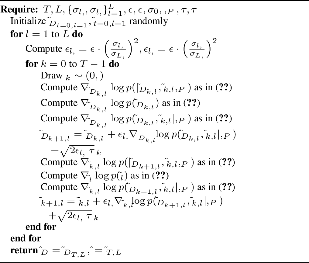
In a nutshell, the algorithm follows these steps: initialization of \(\tilde{\bbX}_{D,0}\) and \(\tilde{\bbH}_0\) randomly. After that, it follows the score function of the joint posterior density of perturbed variables, starting with high \(\sigma_{1, \bbX}\) and \(\sigma_{1, \bbH}\), progressively reducing to \(\sigma_{L, \bbX} \approx \sigma_{L, \bbH} \approx 0\). At early noise levels, the likelihood term directs the dynamics toward an estimate mainly driven by the measurements, while in later noise levels, the prior refines the estimate, as explained further in [13]. Annealing benefits are threefold: it is used to train the score network via score-matching, it enhances dynamic mixing, and it allows for discrete-to-continuous variable approximation. Consequently, we apply annealing to both \(\bbH\) and \(\bbX_D\) to harness the first two benefits for the former and the last two for the latter. With this high-level understanding, we now detail the terms in 7 and provide a step-by-step algorithm description.
Score functions. The score functions are computed with respect to the perturbed variables. Thus, our model for running the dynamic in 5 is described by the following joint posterior distribution \[\label{eq:forwardmodel95noise} p(\tilde{\bbX}_{D,l}, \tilde{\bbH}_l| \bbY, \bbX_P) \propto p( \bbY, \bbX_P |\tilde{\bbX}_{D,l}, \tilde{\bbH}_l)p(\tilde{\bbX}_{D,l})p(\tilde{\bbH}_{l}).\tag{9}\] Hence, we need to compute four score functions 7 , two corresponding to the score of the likelihood terms, and two for the score prior.
i) Score of the likelihood term of \(\tilde{\bbX}_{D,l}\): Under the new model in 9 , the score of the likelihood term for \(\tilde{\bbX}_{D,l}\) is given by \(p(\bbY|\tilde{\bbX}_l, \tilde{\bbH}_l, \bbX_P) = p(\bbZ - \tilde{\bbH}_l {\bbN}_{\bbX,l}|\tilde{\bbX}_{D,l})\), which is not Gaussian: although \(p({\bbN}_{\bbX,l})\) is a Gaussian distribution, after conditioning on the perturbed variable the conditional distribution \(p({\bbN}_{\bbX,l}|\tilde{\bbX}_{D,l})\) is no longer Gaussian. To circumvent this, we consider the following approximation. First, notice that when \(\sigma_{l, \bbX}\) is small, then \(\nabla_{\tilde{\bbX}_D}\log p(\bbY|\tilde{\bbX}_{D,l}, \tilde{\bbH}_l, \bbX_P) \approx \nabla_{\bbX_D}\log p(\bbY_D|\bbX_D, \tilde{\bbH}_l) = \frac{\tilde{\bbH}^{\text{H}}_l(\bbY_D - \tilde{\bbH}_l\bbX_D)}{\sigma_0^2}\), with \(\tilde{\bbH}^{\text{H}}_l\) denoting the conjugate transpose of \(\bbH\); this is only correct when \(\sigma_{l, \bbX} \rightarrow 0\) (recall that for \(\sigma_{l, \bbX} = 0\), the gradient is not defined). Second, given that the approximation is not valid for high \(\sigma_{l, \bbX}\), we add a correction term as follows \[\begin{align} \label{eq:guidance95x} \nabla_{\tilde{\bbX}_D}\log p(\bbY|\tilde{\bbX}_{D,l}, \tilde{\bbH}_l, \bbX_P) &\approx \\\nonumber &\tilde{\bbH}_l^{\text{H}}(\sigma_0^2\bbI + \sigma_{l, \bbX}^2 \tilde{\bbH}_l^{\text{H}}\tilde{\bbH}_l)^{-1}(\bbY_D - \tilde{\bbH}_l\tilde{\bbX}_{D,l}). \end{align}\tag{10}\] Intuitively, the approximation in 10 assumes that the annealing and measurement noise are independent. Although this approximation entails a worse symbol error rate (SER) than the one introduced in [13], it provides a good approximation that allows one to reduce the computational burden of the algorithm.
ii) Score of the likelihood term of \(\tilde{\bbH}_l\): Similar to the approximation in 10 , we approximate the score of likelihood of \(\tilde{\bbH}_l\) as follows \[\label{eq:guidance95H} \nabla_{\tilde{\bbH}_l}\log p(\bbY|\tilde{\bbX}_{D,l}, \tilde{\bbH}_l, \bbX_P) \approx \frac{(\bbY - \tilde{\bbH}_l[\tilde{\bbX}_{D,l}, \bbX_P])[\tilde{\bbX}_{D,l}, \bbX_P]^{\text{H}}}{\sigma_0^2 + \sigma_{l, \bbH}^2}\tag{11}\] Notice that this term considers both the pilots and the data in contrast to the score of the likelihood of \(\tilde{\bbX}_D\) in 10
iii) Score of the annealed prior of \(\tilde{\bbX}_{D,l}\): The score function can be related to the MMSE denoiser through Tweedie’s identity [23] as follows \[\label{eq:prior} \nabla_{\tilde{\bbX}_{D, l}}\log p(\tilde{\bbX}_{D, l}) = \frac{\mathbb{E}_{\sigma_{l, \bbX}}[\bbX_D|\tilde{\bbX}_{D, l}] - \tilde{\bbX}_{D, l}}{\sigma_{l, \bbX}^2}.\tag{12}\] In particular, the conditional expectation can be calculated elementwise as \[\begin{align} \label{E:mixed95gaussian} \mathbb{E}_{\sigma_{l, \bbX}}[x_j|[\tilde{\bbX}_{D, l}]_{j,p}] &= \frac{1}{Z}\sum_{x_k \in \ccalX} x_k \exp\bigg(\frac{-||[\tilde{\bbX}_{D, l}]_{j,p} - x_k||^2}{2\sigma_{l, \bbX}^2}\bigg), \end{align}\tag{13}\] where \(Z = \sum_{x_k \in \ccalX} \exp\Big(\frac{-||[\tilde{\bbX}_{D, l}]_{j,p} - x_k||^2}{2\sigma_{l, \bbX}^2}\Big)\) and \(j=1,\cdots, N_u\).
iv) Score of the annealed prior of \(\tilde{\bbH}_{l}\): Finally, the score prior for \(\tilde{\bbH}_l\) is parameterized by a score network, and trained using denoising score matching, which was introduced in Section 3.1. Hence, \[\begin{align} \label{E:score95network} \nabla_{\tilde{\bbH}_{l}}\log p(\tilde{\bbH}_{l}) = \bbs_{\boldsymbol{\theta}}(\tilde{\bbH}_l, \sigma_{l, \bbH}), \end{align}\tag{14}\] where the network \(\bbs_{\boldsymbol{\theta}}(.)\) is trained by minizing the loss function in 6 .

Figure 1: Annealed Langevin for JED-MAP


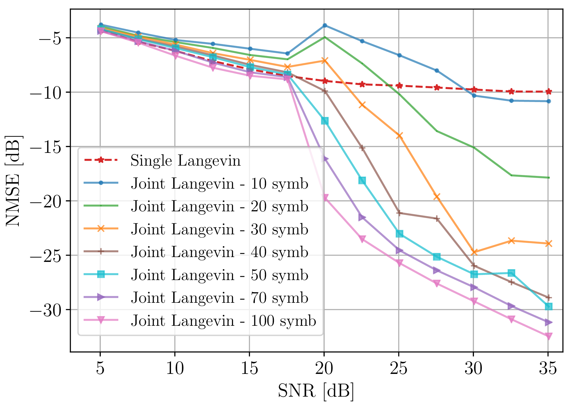
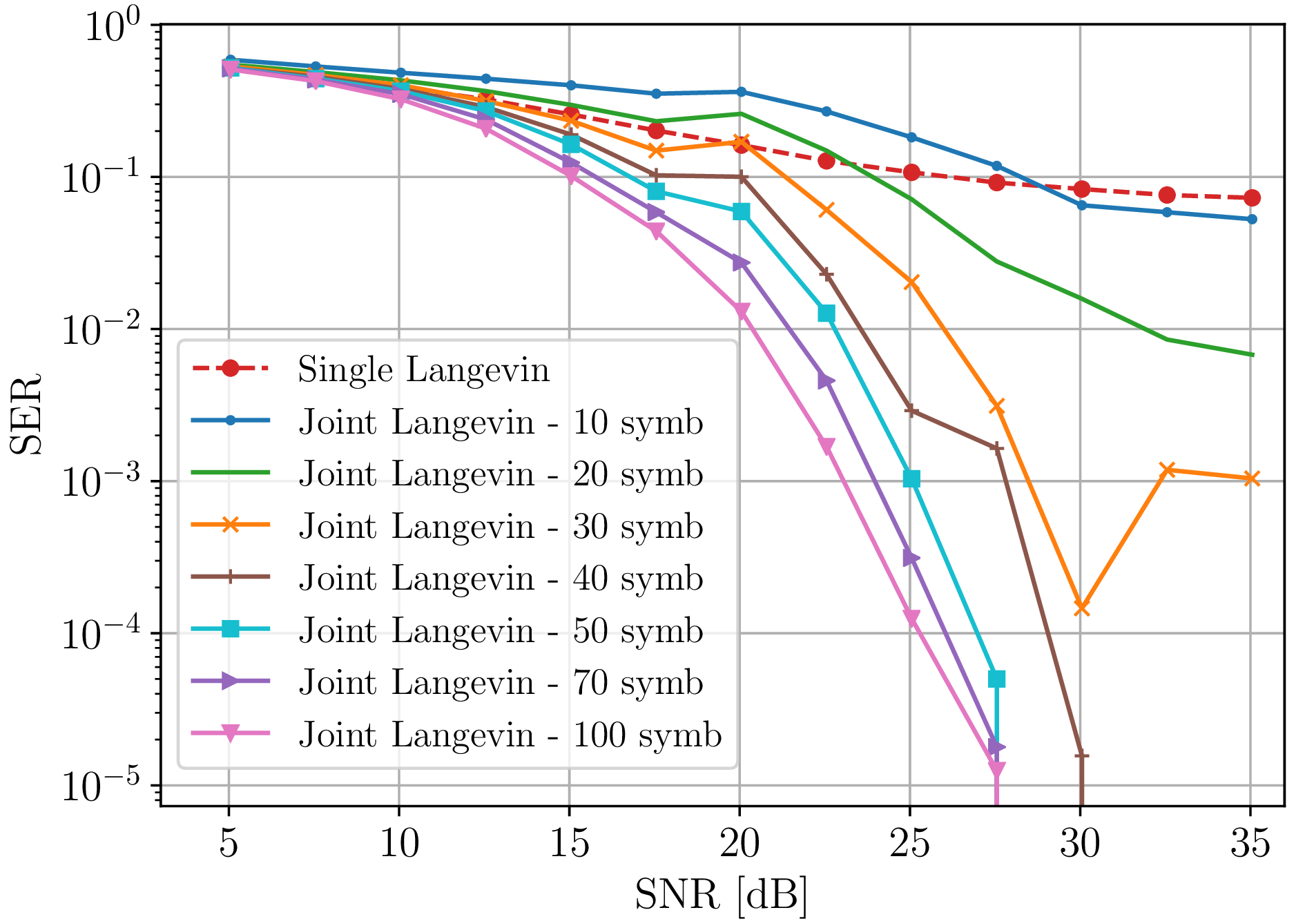
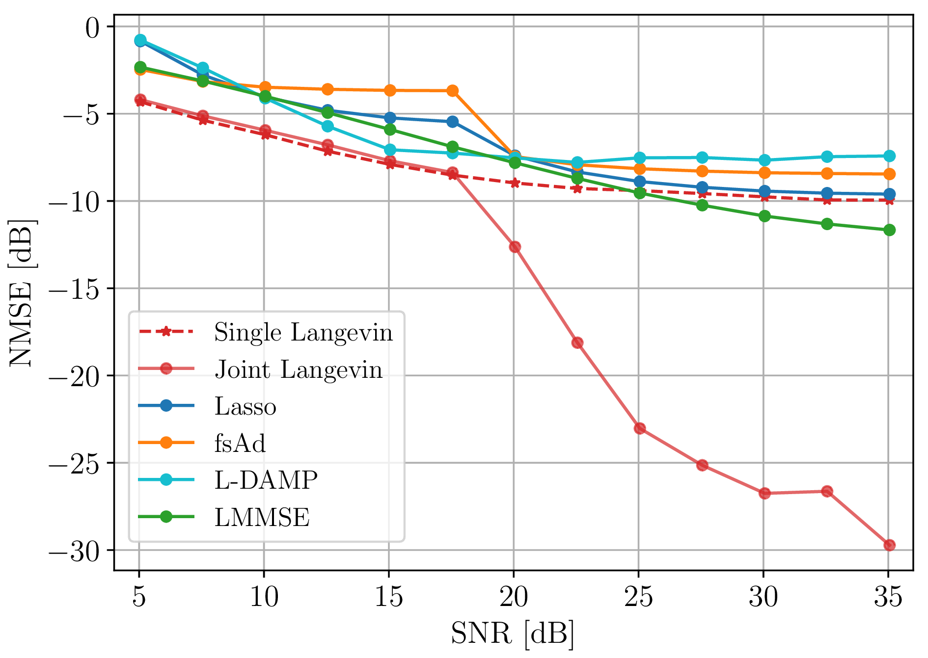
Figure 2: Performance analysis of our proposed method as a function of SNR for a 3GPP channel model. (a), (b) NMSE and SER respectively for a fixed number of pilot symbols \(P = 30\) and different number of data symbols, \(D = \{10, 20, 30, 40, 50, 70, 100\}\). (c) Comparison with different baseline methods, for \(P=30\) and \(D=50\)..
The algorithm to generate estimates \(\hat{\bbH}\) and \(\hat{\bbX}_D\) by sampling from the (approximate) joint posterior \(p(\bbX_D, \bbH|\bbY,\bbX_P)\) is shown in Algorithm 1. From the update steps, we observe that the main advantage of performing joint sampling is to reuse data symbols as pilots, which entails two benefits. First, it allows sending more data with the same data rate and maintaining a given system performance. Second, it reduces the channel estimation error as long as the estimation of the symbols is good. Hence, one might expect to see an improvement at higher SNRs. Finally, from an implementation perspective, the selection of the hyperparameters – the number of levels of noise as well as the step sizes – is key for the stability of the algorithm.
The complexity of Algorithm 1 is the combination of the complexities of each dynamic. The dynamic with respect to the variable \(\bbX_D\) yields a complexity where the main bottleneck is the matrix inversion in 10 . Hence, the complexity of computing the guidance term and the score prior is \(\ccalO(N_u^3 + KN_u)\). A deeper analysis of the complexity of this method can be found in [13]. For the case of \(\bbH\), the heavier computation is carried by the score network. An analysis of the computation complexity of this method can be found in [15].
4 Numerical Experiments↩︎
In this section, we evaluate the performance of our method. 1 We begin by introducing the channel model and simulation setup. The first experiment assesses channel estimation error versus signal-to-noise ratio (SNR), varying the number of symbols \(\bbX_D\) with a fixed pilot count, comparing against the case with no symbol reuse as pilots. In the second experiment, we consider the same setting as experiment one and evaluate the SER as a function of SNR. Finally, we benchmark our approach against baseline methods in channel estimation.
We consider a channel model that is representative of the 3GPP 3D MIMO channel model [24], as implemented in the QuaDRiGa channel simulator [25]. We consider a base station with an \(8\times8\) half-wavelength spacing (\(N_r=64\)), single-polarization antenna array at a height of 20 m. We assume that the BS covers a sector of radius 500 m and \(N_u=32\) single-polarization omni-directional antennas users are dropped randomly in the coverage area. Moreover, users are NLOS and indoors. The carrier frequency is 3.5 GHz, and each subcarrier has a 100 MHz bandwidth. The spacing within subcarriers is 30 kHz. For the score network, we use the parameterization proposed in [26], and minimize the loss in 6 . We consider a training dataset with \(7000\) channels, and a validation set of \(2500\) channels. We evaluate the performance in a batch size of \(50\) matrices. For the pilots, we generate \(P\) QPSK symbols. The parameters of the Algorithm 1 are \(L = 2311, T = 3, \epsilon_{\bbH} = 1 \times 10^{-10}, \tau_{\bbH} = 1\times 10^{-3}\) and \([\sigma_{1,\bbH}, \sigma_{L, \bbH}] = [30, 0.001]\); lastly, for the dynamic with respect to \(\bbX_D\), we use two different values depending on the SNR: for low SNR (5 db-15 db) we consider \(\epsilon_{\bbX} = 1 \times 10^{-4}, \tau_{\bbX} = 0.5\) and \([\sigma_{1,\bbX}, \sigma_{L, \bbX}] = [0.6,0.01 ]\), while for all other SNR values we fixed \(\epsilon_{\bbX} = 4 \times 10^{-5}, \tau_{\bbX} = 0.1\) and \([\sigma_{1,\bbX}, \sigma_{L, \bbX}] = [0.8,0.01]\). Lastly, the noise variance \(\sigma_0^2\) changes for different levels of SNR. If computationally limiting, \(L\) can be reduced by considering higher-order Langevin dynamics; see [27] for an analysis of the case of channel sampling.
In this first experiment, we analyze the performance of our proposed algorithm for channel estimation with different values for \(D\), i.e., symbols to reuse as pilots, and fixing the value of \(P = 30\). The comparison is shown in Fig. 2 (a), where we named single Langevin the channel sampling for \(D = 0\), proposed in [15]. As expected, performance improves with an increasing number of data symbols for pilot reuse. Notably, when \(D > 30\), our method excels for SNRs above 20 db, and for \(D > 50\), it outperforms single Langevin across all SNRs. Overall, superior performance is evident for SNRs higher than 20 db.
In the same experimental conditions as before (where \(P = 30\)), we examine the SER as a function of SNR, with varying values of \(D\). The results are presented in Fig. 2 (b). Similar to the behavior observed in channel estimation error, we notice an improvement in SER as \(D\) increases. Notably, when \(D > 30\), our proposed algorithm outperforms the single Langevin method across all SNRs. These findings suggest that the limitation in NMSE performance in our algorithm stems from symbol sampling performance. In high SNR scenarios, accurate estimation of \(\bbX_D\) leads to precise joint variable estimation. However, in lower SNR situations, there is not a significant advantage in considering symbol reuse.
In our third experiment, we compare our proposed algorithm to several baseline methods: LASSO [28], fsAD [29], L-MMSE [30], L-DAMP [31], and Langevin using only pilots [15]. We set \(P = 30\) for all baseline algorithms and \(D = 50\) for our method. Results in Fig. 2 (c) reveal that our approach consistently outperforms all baselines across all SNRs. Particularly noteworthy is its superior performance, exceeding other methods by several orders of magnitude for SNRs above 15 db.
5 Conclusions↩︎
We introduced an algorithm for joint massive MIMO channel estimation and data detection using diffusion models. Our approach leverages the reverse processes to generate samples for solving the MAP-JED optimization problem, accommodating both discrete and continuous variable priors. Simulations reveal our method’s superior performance over baselines while managing pilot overhead. Future work aims to explore streamlined diffusion models, reducing hyperparameters and accelerating sampling, and enhancing performance in lower SNR scenarios.
References↩︎
Code for reproducing experiments is available at https://github.com/nzilberstein/Langevin-joint-channel↩︎