Keywords: federated reinforcement learning, multi-task reinforcement learning, natural policy gradient methods, entropy regularization, dimension-free global convergence

1 Introduction↩︎

Federated reinforcement learning (FRL) is an emerging paradigm that combines the advantages of federated learning (FL) and reinforcement learning (RL) [1], [2], allowing multiple agents to learn a shared policy from local experiences, without exposing their private data to a central server nor other agents. FRL is poised to enable collaborative and efficient decision making in scenarios where data is distributed, heterogeneous, and sensitive, which arise frequently in applications such as edge computing, smart cities, and healthcare [2]–[4], to name just a few. As has been observed [5], decentralized training can lead to performance improvements in FL by avoiding communication congestions at busy nodes such as the server, especially under high-latency scenarios. This motivates us to design algorithms for the fully decentralized setting, a scenario where the agents can only communicate with their local neighbors over a prescribed network topology.⁶

In this work, we study the problem of federated multi-task reinforcement learning [1], [6], [7], where each agent collects its own reward — possibly unknown to other agents — corresponding to the local task at hand, while having access to the same dynamics (i.e., transition kernel) of the environment. The collective goal is to learn a shared policy that maximizes the total rewards accumulated from all the agents; in other words, one seeks a policy that performs well in terms of overall benefits, rather than biasing towards any individual task, achieving the Pareto frontier in a multi-objective context. There is no shortage of application scenarios where federated multi-task RL becomes highly relevant. For instance, in healthcare [8], different hospitals may be interested in finding an optimal treatment for all patients without disclosing private data, where the effectiveness of the treatment can vary across different hospitals due to demographical differences. As another potential application, to enhance ChatGPT’s performance across different tasks or domains [9], [10], one might consult domain experts to chat and rate ChatGPT’s outputs for solving different tasks, and train ChatGPT in a federated manner without exposing private data or feedback of each expert.

Nonetheless, despite the promise, provably efficient algorithms for federated multi-task RL remain substantially under-explored, especially in the fully decentralized setting. The heterogeneity of local tasks leads to a higher degree of disagreements between the global value function and local value functions of individual agents. Due to the lack of global information sharing, care needs to be taken to judiciously balance the use of neighboring information (to facilitate consensus) and local data (to facilitate learning) when updating the policy. To the best of our knowledge, very limited algorithms are currently available to find the global optimal policy with non-asymptotic convergence guarantees even for tabular infinite-horizon Markov decision processes.

Motivated by the connection with decentralized optimization, it is tempting to take a policy optimization perspective to tackle this challenge. Policy gradient (PG) methods, which seek to learn the policy of interest via first-order optimization methods, play an eminent role in RL due to their simplicity and scalability. In particular, natural policy gradient (NPG) methods [11], [12] are among the most popular variants of PG methods, underpinning default methods used in practice such as trust region policy optimization (TRPO) [13] and proximal policy optimization (PPO) [14]. On the theoretical side, it has also been established recently that the NPG method enjoys fast global convergence to the optimal policy in an almost dimension-free manner [15], [16], where the iteration complexity is nearly independent of the size of the state-action space. These benefits can be translated to their sample-based counterparts such as the natural actor critic (NAC) method [17], where the value functions are learned via temporal difference learning. Inspired by the efficacy of NPG methods, it is natural to ask:

1.1 Our contributions↩︎

Focusing on infinite-horizon Markov decision processes (MDPs), we provide an affirmative answer to the above question, by developing federated NPG (FedNPG) methods for solving both the vanilla and entropy-regularized multi-task RL problems with finite-time global convergence guarantees. While entropy regularization is often incorporated as an effective strategy to encourage exploration during policy learning, solving the entropy-regularized RL problem is of interest in its own right, as the optimal regularized policy possesses desirable robust properties with respect to reward perturbations [18], [19].

Due to the multiplicative update nature of NPG methods under softmax parameterization, it is more convenient to work with the logarithms of local policies in the decentralized setting. In each iteration of the proposed FedNPG method, the logarithms of local policies are updated by a weighted linear combination of two terms (up to normalization): a gossip mixing [20] of the logarithms of neighboring local policies, and a local estimate of the global Q-function tracked via the technique of dynamic average consensus [21], a prevalent idea in decentralized optimization that allows for the use of large constant learning rates [22]–[24] to accelerate convergence. We further develop sample-efficient federated NAC (FedNAC) methods that allow for both stochastic updates and function approximation. Our contributions are as follows.

• We propose FedNPG methods for both the vanilla and entropy-regularized multi-task RL problems, where each agent only communicates with its neighbors and performs local computation using its own reward or task information.

• Assuming access to exact policy evaluation, we establish that the average iterate of vanilla FedNPG converges globally at a rate of \(\mathcal{O}(1/T^{2/3})\) in terms of the sub-optimality gap for the multi-task RL problem, and that the last iterate of entropy-regularized FedNPG converges globally at a linear rate to the regularized optimal policy. Our convergence theory highlights the impacts of all salient problem parameters (see Table ¿tbl:tb:iteration95complexity? for details), such as the size and connectivity of the communication network. In particular, the iteration complexities of FedNPG are again almost independent of the size of the state-action space, which recover prior results on the centralized NPG methods when the network is fully connected.

• We further demonstrate the stability of the proposed FedNPG methods when policy evaluations are only available in an inexact manner. To be specific, we prove that their convergence rates remain unchanged as long as the approximation errors are sufficiently small in the \(\ell_\infty\) sense.

• We go beyond the tabular setting by proposing FedNAC— a federated actor critic method for multi-task RL with function approximation — and establish a finite-sample sample complexity on the order of \(\mathcal{O}(1/\varepsilon^{7/2})\) for each agent in terms of the expected sub-optimality gap.

To the best of our knowledge, the proposed federated NPG and NAC methods are the first policy optimization methods for multi-task RL that achieve near dimension-free global convergence guarantees in terms of iteration and sample complexities, allowing for fully decentralized communication without any need to share local reward/task information.

1.2 Related work↩︎

1.2.0.1 Global convergence of NPG methods for tabular MDPs.

[15] first establishes a \(\mathcal{O}(1/T)\) last-iterate convergence rate of the NPG method under softmax parameterization with constant step size, assuming access to exact policy evaluation. When entropy regularization is in place, [16] establishes a global linear convergence to the optimal regularized policy for the entire range of admissible constant learning rates using softmax parameterization and exact policy evaluation, which is further shown to be stable in the presence of \(\ell_\infty\) policy evaluation errors. The iteration complexity of NPG methods is nearly independent with the size of the state-action space, which is in sharp contrast to softmax policy gradient methods that may take exponential time to converge [25], [26]. [27] proposed a more general framework through the lens of mirror descent for regularized RL with global linear convergence guarantees, which is further generalized in [28], [29]. Earlier analysis of regularized MDPs can be found in [30]. Besides, [31] proves that vanilla NPG also achieves linear convergence when geometrically increasing learning rates are used; see also [32], [33]. [34] developed an anchor-changing NPG method for multi-task RL under various optimality criteria in the centralized setting.

1.2.0.2 Convergence and sample complexity bounds of NAC.

The convergence and sample complexity of a variety of natural actor-critic methods (NACs) are extensively studied in the literature [15], [35]–[38]. More pertinent to our work, [15] introduced Q-NPG — a sample version of the NPG method with function approximation under softmax parameterization — and obtained a convergence rate of \(\mathcal{O}(1/\sqrt{T})\). [38] weakens some of its assumptions and improves the convergence rate to \(\mathcal{O}(1/T)\) and gives the \(\widetilde{\mathcal{O}}(1/\varepsilon^3)\) sample complexity using a constant actor learning rate. The FedNAC method we propose in this paper can be seen as a decentralized version of Q-NPG, and in the server-client setting where the network is fully connected, our convergence rate and sample complexity match those in [38].

1.2.0.3 Distributed and federated RL.

There have been a variety of settings being set forth for distributed and federated RL. [39]–[43] focused on developing federated versions of RL algorithms to accelerate training, assuming all agents share the same transition kernel and reward function; in particular, [42]–[44] established the provable benefits of federated learning in terms of linear speedup. More pertinent to our work, [6], [45] considered the federated multi-task framework, allowing different agents having private reward functions. [45] proposed an empirically probabilistic algorithm that can seek an optimal policy under the server-client setting, while [6] developed new attack methods in the presence of adversarial agents. Recently [46] discussed how to avoid transmitting the Hessian matrix during communication in the server-client setting where all agents share the same reward function. Different from the FRL framework, [47]–[52] considered the distributed multi-agent RL setting where the agents interact with a dynamic environment through a multi-agent Markov decision process, where each agent can have their own state or action spaces. [52] developed a decentralized policy gradient method where different agents have different MDPs, where a special case of their setting recovers ours. However, the convergence rate developed in [52] has rather pessimistic dependencies with the size of the state-action space, together with other parameters, without leveraging natural policy gradients and gradient tracking techniques.

1.2.0.4 Decentralized first-order optimization algorithms.

Early work of consensus-based first-order optimization algorithms for the fully decentralized setting include but are not limited to [20], [53], [54]. Gradient tracking, which leverages the idea of dynamic average consensus [21] to track the gradient of the global objective function, is a popular method to improve the convergence speed [22]–[24], [55], [56].

1.2.0.5 Notation.

Boldface small and capital letters denote vectors and matrices, respectively. Sets are denoted with curly capital letters, e.g., \({\mathcal{S}},{\mathcal{A}}\). We let \(({\mathbb{R}}^d,\left\| \cdot \right\|)\) denote the \(d\)-dimensional real coordinate space equipped with norm \(\left\| \cdot \right\|\). The \(\ell^p\)-norm of \({\boldsymbol{v}}\) is denoted by \(\left\| {\boldsymbol{v}} \right\|_p\), where \(1\leq p\leq \infty\), and the spectral norm and the Frobenius norm of a matrix \({\boldsymbol{M}}\) are denoted by \(\left\| {\boldsymbol{M}} \right\|_2\) and \(\left\| {\boldsymbol{M}} \right\|_F\), resp. We let \([N]\) denote \(\{1, \dots, N\}\), use \({\boldsymbol{1}}_N\) to represent the all-one vector of length \(N\), and denote by \({\boldsymbol{0}}\) a vector or a matrix consisting of all 0’s. We allow the application of functions such as \(\log(\cdot)\) and \(\exp(\cdot)\) to vectors or matrices, with the understanding that they are applied in an element-wise manner.

2 Model and backgrounds↩︎

2.1 Markov decision processes↩︎

2.1.0.1 Markov decision processes.

We consider an infinite-horizon discounted Markov decision process (MDP) denoted by \(\mathcal{M} = (\mathcal{S}, \mathcal{A}, P, r, \gamma)\), where \(\mathcal{S}\) and \(\mathcal{A}\) denote the state space and the action space, respectively, \(\gamma\in [0, 1)\) indicates the discount factor, \(P: \mathcal{S}\times \mathcal{A} \rightarrow \Delta(\mathcal{S})\) is the transition kernel, and \(r: \mathcal{S}\times \mathcal{A} \rightarrow [0, 1]\) stands for the reward function. To be more specific, for each state-action pair \((s, a) \in \mathcal{S}\times \mathcal{A}\) and any state \(s' \in \mathcal{S}\), we denote by \(P(s'|s, a)\) the transition probability from state \(s\) to state \(s'\) when action \(a\) is taken, and \(r(s, a)\) the instantaneous reward received in state \(s\) when action \(a\) is taken. Furthermore, a policy \(\pi : \mathcal{S} \rightarrow \Delta(\mathcal{A})\) specifies an action selection rule, where \(\pi(a|s)\) specifies the probability of taking action \(a\) in state \(s\) for each \((s, a) \in \mathcal{S}\times \mathcal{A}\).

For any given policy \(\pi\), we denote by \(V^\pi : \mathcal{S} \mapsto {\mathbb{R}}\) the corresponding value function, which is the expected discounted cumulative reward with an initial state \(s_0 = s\), given by \[\label{eq:V} \forall s\in \mathcal{S}: \quad V^\pi (s) \mathrel{\vcenter{:}}= \mathbb{E}\left[\sum_{t=0}^\infty \gamma^t r(s_t,a_t)| s_0=s\right],\tag{1}\] where the randomness is over the trajectory generated following the policy \(a_t \sim \pi(\cdot|s_t)\) and the MDP dynamic \(s_{t+1} \sim P(\cdot|s_t, a_t)\). We also overload the notation \(V^\pi (\rho)\) to indicate the expected value function of policy \(\pi\) when the initial state follows a distribution \(\rho\) over \(\mathcal{S}\), namely, \(V^\pi (\rho) \mathrel{\vcenter{:}}= \mathbb{E}_{s\sim \rho}\left[V^\pi(s)\right]\). Similarly, the Q-function \(Q^\pi : \mathcal{S} \times \mathcal{A} \mapsto \mathbb{R}\) of policy \(\pi\) is defined by \[\label{eq:Q} \forall (s,a)\in \mathcal{S}\times \mathcal{A}:\quad Q^\pi (s,a)\mathrel{\vcenter{:}}= \mathbb{E}\left[\sum_{t=0}^\infty \gamma^t r(s_t,a_t)| s_0=s, a_0=a\right],\tag{2}\] which measures the expected discounted cumulative reward with an initial state \(s_0 = s\) and an initial action \(a_0 = a\), with expectation taken over the randomness of the trajectory. The optimal policy \(\pi^{\star}\) refers to the policy that maximizes the value function \(V^{\pi}(s)\) for all states \(s\in{\mathcal{S}}\), which is guaranteed to exist [57]. The corresponding optimal value function and Q-function are denoted as \(V^{\star}\) and \(Q^{\star}\), respectively.

2.2 Entropy-regularized RL↩︎

Entropy regularization [58], [59] is a popular technique in practice that encourages stochasticity of the policy to promote exploration, as well as robustness against reward uncertainties. Mathematically, this can be viewed as adjusting the instantaneous reward based the current policy in use as \[\label{eq:reward95reg} \forall (s,a)\in \mathcal{S}\times \mathcal{A}:\quad r_\tau(s,a)\mathrel{\vcenter{:}}= r(s,a)-\tau \log{\pi (a|s)}\,,\tag{3}\] where \(\tau\geq 0\) denotes the regularization parameter. Typically, \(\tau\) should not be too large to outweigh the actual rewards; for ease of presentation, we assume \(\tau\leq \min\left\{1, \, \frac{1}{\log| \mathcal{A}|} \right\}\) [60]. Equivalently, this amounts to the entropy-regularized (also known as “soft”) value function, defined as \[\label{eq:V95reg95s} \forall s\in \mathcal{S}: \quad V_\tau^\pi (s) \mathrel{\vcenter{:}}= V^\pi (s) +\tau \mathcal{H}(s,\pi).\tag{4}\] Here, we define \[\begin{align} \mathcal{H}(s,\pi)& \mathrel{\vcenter{:}}= \mathbb{E}\left[\sum_{t=0}^\infty -\gamma^t \log{\pi (a_t|s_t)}\big | s_0=s\right] =\frac{1}{1-\gamma}\mathbb{E}_{s'\sim d_s^\pi}\left[ - \sum_{a\in\mathcal{A}}\pi(a|s')\log \pi(a|s')\right] , \label{eq:entropy95reg95s} \end{align}\tag{5}\] where \(d^\pi_{s_0}\) is the discounted state visitation distribution of policy \(\pi\) given an initial state \(s_0 \in \mathcal{S}\), denoted by \[\label{eq:d95s0} \forall s\in\mathcal{S}: \quad d^\pi_{s_0}(s)\mathrel{\vcenter{:}}= (1-\gamma)\sum_{t=0}^\infty \gamma^t\mathbb{P}(s_t=s|s_0)\,,\tag{6}\] with the trajectory generated by following policy \(\pi\) in the MDP \(\mathcal{M}\) starting from state \(s_0\). Analogously, the regularized (or soft) Q-function \(Q_\tau^\pi\) of policy \(\pi\) is related to the soft value function \(V_\tau^\pi(s)\) as \[\begin{align} \forall (s,a)\in \mathcal{S}\times \mathcal{A}:\quad Q_\tau^\pi(s,a)&=r(s,a)+\gamma\mathbb{E}_{s'\in P(\cdot|s,a)}\left[V_\tau^\pi(s')\right]\,,\tag{7}\\ \forall s\in \mathcal{S}:\quad V_\tau^\pi (s)&=\mathbb{E}_{a\sim \pi(\cdot|s)}\left[-\tau\pi(a|s)+Q_\tau^\pi(s,a)\right]\,.\tag{8} \end{align}\] The optimal regularized policy, the optimal regularized value function, and the Q-function are denoted by \(\pi^\star_\tau\), \(V^\star_\tau\), and \(Q^\star_\tau\), respectively.

For a distribution \(\rho\in\Delta({\mathcal{S}})\), we define \(d_\rho^\pi(s)=\mathbb{E}_{s_0\sim\rho}[d_{s_0}^\pi(s)]\). We also define the state-action visitation distribution \(\bar{d}^\pi_\rho\) as \[\label{eq:sa95vis} \forall (s,a)\in{\mathcal{S}}\times {\mathcal{A}}:\quad \bar{d}^\pi_{\rho}(s,a)\mathrel{\vcenter{:}}= d^\pi_{\rho}(s)\pi(a|s)=(1-\gamma)\mathbb{E}_{s_0\sim\rho}\left[\sum_{t=0}^\infty \gamma^t\mathbb{P}(s_t=s, a_t=a|s_0)\right].\tag{9}\] Furthermore, we define the state-action visitation distribution induced by an initial state-action distribution \(\nu\in\Delta({\mathcal{S}}\times{\mathcal{A}})\), i.e., \[\label{eq:sa95vis95extend} \forall (s,a)\in{\mathcal{S}}\times {\mathcal{A}}:\quad \tilde{d}^\pi_{\nu}(s,a)\mathrel{\vcenter{:}}= (1-\gamma)\mathbb{E}_{(s_0,a_0)\sim\nu}\left[\sum_{t=0}^\infty \gamma^t\mathbb{P}(s_t=s, a_t=a|s_0,a_0)\right].\tag{10}\]

The following simple fact holds for all \((s,a)\in{\mathcal{S}}\times{\mathcal{A}}\): \[\label{eq:d95facts} d_\rho^\pi(s)\geq (1-\gamma)\rho(s),\quad \bar{d}^\pi_{\rho}(s,a)\geq (1-\gamma)\rho(s)\pi(a|s),\quad \tilde{d}^\pi_{\nu}(s,a)\geq (1-\gamma)\nu(s,a).\tag{11}\]

2.3 Natural policy gradient methods↩︎

Natural policy gradient (NPG) methods lie at the heart of policy optimization, serving as the backbone of popular heuristics such as TRPO [13] and PPO [14]. Instead of directly optimizing the policy over the probability simplex, one often adopts the softmax parameterization, which parameterizes the policy as \[\label{eq:softmax95policy} \pi_\theta \mathrel{\vcenter{:}}= \mathrm{softmax}(\theta) \quad \text{or} \quad \forall (s,a)\in \mathcal{S}\times \mathcal{A}: \quad \pi_\theta(a|s)\mathrel{\vcenter{:}}= \frac{\exp{\theta(s,a)}}{\sum_{a'\in \mathcal{A}}\exp{\theta(s,a')}}\tag{12}\] for any \(\theta\): \(\mathcal{S}\times \mathcal{A} \rightarrow \mathbb{R}\).

2.3.0.1 Vanilla NPG method.

In the tabular setting, the update rule of vanilla NPG at the \(t\)-th iteration can be concisely represented as \[\label{eq:update95npg95vanilla} \forall (s,a)\in \mathcal{S}\times \mathcal{A}:\quad \pi^{(t+1)}(a|s) \propto \pi^{(t)}(a|s) \exp{\left(\frac{\eta Q^{(t)}(s,a)}{1-\gamma}\right)}\,,\tag{13}\] where \(\eta>0\) denotes the learning rate, and \(Q^{(t)} = Q^{\pi^{(t)}}\) is the Q-function under policy \(\pi^{(t)}\). [15] shows that: in order to find an \(\varepsilon\)-optimal policy, NPG takes at most \(\mathcal{O}\left(\frac{1}{(1-\gamma)^2\varepsilon} \right)\) iterations, assuming exact policy evaluation.

2.3.0.2 Entropy-regularized NPG method.

Turning to the regularized problem, we note that the update rule of entropy-regularized NPG becomes \[\label{eq:update95npg} \forall (s,a)\in \mathcal{S}\times \mathcal{A}:\quad \pi^{(t+1)}(a|s) \propto (\pi^{(t)}(a|s))^{1-\frac{\eta\tau}{1-\gamma}}\exp{\left(\frac{\eta Q_\tau^{(t)}(s,a)}{1-\gamma}\right)}\,,\tag{14}\] where \(\eta\in (0,\frac{1-\gamma}{\tau}]\) is the learning rate, and \(Q_{\tau}^{(t)} = Q_{\tau}^{\pi^{(t)}}\) is the soft Q-function of policy \(\pi^{(t)}\). [61] proves that entropy-regularized NPG enjoys fast global linear convergence to the optimal regularized policy: to find an \(\varepsilon\)-optimal regularized policy, entropy-regularized NPG takes no more than \(\mathcal{O}\left(\frac{1}{\eta\tau}\log \left(\frac{1}{\varepsilon}\right)\right)\) iterations.

3 Federated NPG methods for multi-task RL↩︎

3.1 Federated multi-task RL↩︎

In this paper, we consider the federated multi-task RL setting, where a set of agents learn collaboratively a single policy that maximizes its average performance over all the tasks using only local computation and communication.

3.1.0.1 Multi-task RL.

Each agent \(n\in [N]\) has its own private reward function \(r_n(s,a)\) — corresponding to different tasks — while sharing the same transition kernel of the environment. The goal is to collectively learn a single policy \(\pi\) that maximizes the global value function given by \[\label{eq:global95V} V^{\pi}(s) = \frac{1}{N}\sum_{n=1}^N V_n^{\pi}(s) ,\tag{15}\] where \(V_n^\pi\) is the value function of agent \(n\in[N]\), defined by \[\label{eq:V95n} \forall s\in \mathcal{S}: \quad V_n^\pi (s)\mathrel{\vcenter{:}}= \mathbb{E}\left[\sum_{t=0}^\infty \gamma^t r_n(s_t,a_t)| s_0=s\right]\,.\tag{16}\] Clearly, the global value function 15 corresponds to using the average reward of all agents \[\label{eq:global95r} r(s, a)=\frac{1}{N}\sum_{n=1}^N r_n(s,a).\tag{17}\] The global Q-function \(Q^{\pi}(s,a)\) and the agent Q-functions \(Q_n^{\pi}(s,a)\) can be defined in a similar manner obeying \(Q^\pi(s,a)=\frac{1}{N}\sum_{n=1}^N Q_n^\pi(s,a)\).

In parallel, we are interested in the entropy-regularized setting, where each agent \(n\in[N]\) is equipped with a regularized reward function given by \[\label{eq:reward95reg95n} r_{\tau,n}(s,a) \mathrel{\vcenter{:}}= r_n(s,a)-\tau \log{\pi (a|s)}\,,\tag{18}\] and we define similarly the regularized value function and the global regularized value function as \[\label{eq:V95reg95n} \forall s\in \mathcal{S}: \quad V_{\tau,n}^\pi (s) \mathrel{\vcenter{:}}= \mathbb{E}\left[\sum_{t=0}^\infty \gamma^t r_{\tau,n}(s_t,a_t)| s_0=s\right]\,, \quadand\quad V_\tau^\pi(s)=\frac{1}{N}\sum_{n=1}^N V_{\tau,n}^\pi(s).\tag{19}\] The soft Q-function of agent \(n\) is given by \[\label{eq:Q95reg95n} Q_{\tau,n}^\pi(s,a)=r_{n}(s,a)+\gamma\mathbb{E}_{s'\in P(\cdot|s,a)}\left[V_{\tau,n}^\pi(s')\right]\,,\tag{20}\] and the global soft Q-function is given by \(Q_\tau^\pi(s,a)=\frac{1}{N}\sum_{n=1}^N Q_{\tau,n}^\pi(s,a)\).

3.1.0.2 Federated policy optimization in the fully decentralized setting.

We consider a federated setting with fully decentralized communication, that is, all the agents are synchronized to perform information exchange over some prescribed network topology denoted by an undirected weighted graph \(\mathcal{G}([N],E)\). Here, \(E\) stands for the edge set of the graph with \(N\) nodes — each corresponding to an agent — and two agents can communicate with each other if and only if there is an edge connecting them. The information sharing over the graph is best described by a mixing matrix [20], denoted by \({\boldsymbol{W}}=[w_{ij}]\in[0,1]^{N\times N}\), where \(w_{ij}\) is a positive number if \((i,j)\in E\) and 0 otherwise. We also make the following standard assumptions on the mixing matrix.

The following standard metric measures how fast information propagates over the graph.

The spectral radius \(\sigma\) determines how fast information propagate over the network. For instance, in a fully-connected network, we can achieve \(\sigma = 0\) by setting \({\boldsymbol{W}}= \frac{1}{N}{\boldsymbol{1}}_N{\boldsymbol{1}}_N^\top\). For control of \(1/(1 - \sigma)\) regarding different graphs, we refer the readers to paper [62]. In an Erdös-Rényi random graph, as long as the graph is connected, one has with high probability \(\sigma \asymp 1\). Another immediate consequence is that for any \({\boldsymbol{x}}\in\mathbb{R}^N\), letting \(\overline{x}=\frac{1}{N}{\boldsymbol{1}}_N^\top{\boldsymbol{x}}\) be its average, we have \[\label{eq:property95W} \left\| {\boldsymbol{W}}{\boldsymbol{x}}-\overline{x}{\boldsymbol{1}}_N \right\|_2\leq\sigma \left\| {\boldsymbol{x}}-\overline{x}{\boldsymbol{1}}_N \right\|_2\,,\tag{21}\] where the consensus error contracts by a factor of \(\sigma\).

3.2 Proposed federated NPG algorithms↩︎

Assuming softmax parameterization, the problem can be formulated as decentralized optimization, \[\begin{align} \textsf{(unregularized)} \qquad \max_{\theta} \; V^{\pi_\theta}(s) = \frac{1}{N}\sum_{n=1}^N V_n^{\pi_\theta}(s) , \tag{22} \\ \textsf{(regularized)} \qquad \max_{\theta} \; V_{\tau}^{\pi_\theta}(s) = \frac{1}{N}\sum_{n=1}^N V_{\tau,n}^{\pi_\theta}(s) , \tag{23} \end{align}\] where \(\pi_\theta \mathrel{\vcenter{:}}= \mathrm{softmax}(\theta)\) subject to communication constraints. Motivated by the success of NPG methods, we aim to develop federated NPG methods to achieve our goal. For notational convenience, let \({\boldsymbol{\pi}}^{(t)} \mathrel{\vcenter{:}}= \big(\pi_1^{(t)},\cdots,\pi_N^{(t)} \big)^\top\) be the collection of policy estimates at all agents in the \(t\)-th iteration. Let \[\label{eq:average95policy} \overline{\pi}^{(t)} \mathrel{\vcenter{:}}= \mathrm{softmax}\left(\frac{1}{N}\sum_{n=1}^N \log \pi_n^{(t)}\right),\tag{24}\] which satisfies that \(\overline{\pi}^{(t)}(a|s)\propto \left(\prod_{n=1}^N \pi_n^{(t)}(a|s)\right)^{1/N}\) for each \((s,a)\in \mathcal{S}\times \mathcal{A}\). Therefore, \(\overline{\pi}^{(t)}\) could be seen as the normalized geometric mean of \(\{\pi_n^{(t)}\}_{n\in[N]}\). Define the collection of Q-function estimates as \[\begin{align} {\boldsymbol{Q}}^{(t)} \mathrel{\vcenter{:}}= \Big( Q_{1}^{\pi_1^{(t)}},\cdots, Q_{N}^{\pi_N^{(t)}}\Big)^\top , \qquad {\boldsymbol{Q}}_\tau^{(t)} \mathrel{\vcenter{:}}= \Big( Q_{\tau,1}^{\pi_1^{(t)}},\cdots, Q_{\tau,N}^{\pi_N^{(t)}}\Big)^\top. \end{align}\] We shall often abuse the notation and treat \({\boldsymbol{\pi}}^{(t)}\), \({\boldsymbol{Q}}_\tau^{(t)}\) as matrices in \(\mathbb{R}^{N\times |\mathcal{S}||\mathcal{A}|}\), and treat \({\boldsymbol{\pi}}^{(t)}(a|s)\), \({\boldsymbol{Q}}_\tau^{(t)}(a|s)\) as vectors in \(\mathbb{R}^N\), for all \((s,a)\in \mathcal{S}\times\mathcal{A}\).

3.2.0.1 Vanilla federated NPG methods.

To motivate the algorithm development, observe that the NPG method (cf. 13 ) applied to 22 adopts the update rule \[\begin{align} \pi^{(t+1)}(a|s) \propto \pi^{(t)}(a|s) \exp{\left(\frac{\eta Q^{\pi^{(t)}}(s,a)}{1-\gamma}\right)} = \pi^{(t)}(a|s) \exp{\left(\frac{\eta \sum_{n=1}^N Q_n^{\pi^{(t)}}(s,a)}{N(1-\gamma)}\right)} \, \end{align}\] for all \((s,a)\in \mathcal{S}\times \mathcal{A}\). Two challenges arise when executing this update rule: the policy estimates are maintained locally without consensus, and the global Q-function are unavailable in the decentralized setting. To address these challenges, we apply the idea of dynamic average consensus [21], where each agent maintains its own estimate \(T_n^{(t)}(s,a)\) of the global Q-function, which are collected as vector \[{\boldsymbol{T}}^{(t)} = \big( T_{1}^{(t)},\cdots, T_{N}^{ (t)}\big)^\top.\] At each iteration, each agent updates its policy estimates based on its neighbors’ information via gossip mixing, in addition to a correction term that tracks the difference \(Q_n^{\pi_n^{(t+1)}}(s,a) - Q_n^{\pi_n^{(t)}}(s,a)\) of the local Q-functions between consecutive policy updates. Note that the mixing is applied linearly to the logarithms of local policies, which translates into a multiplicative mixing of the local policies. Algorithm 1 summarizes the detailed procedure of the proposed algorithm written in a compact matrix form, which we dub as federated NPG (FedNPG). Note that the agents do not need to share their reward functions with others, and agent \(n\in [N]\) will only be responsible to evaluate the local policy \(\pi_n^{(t)}\) using the local reward \(r_n\).

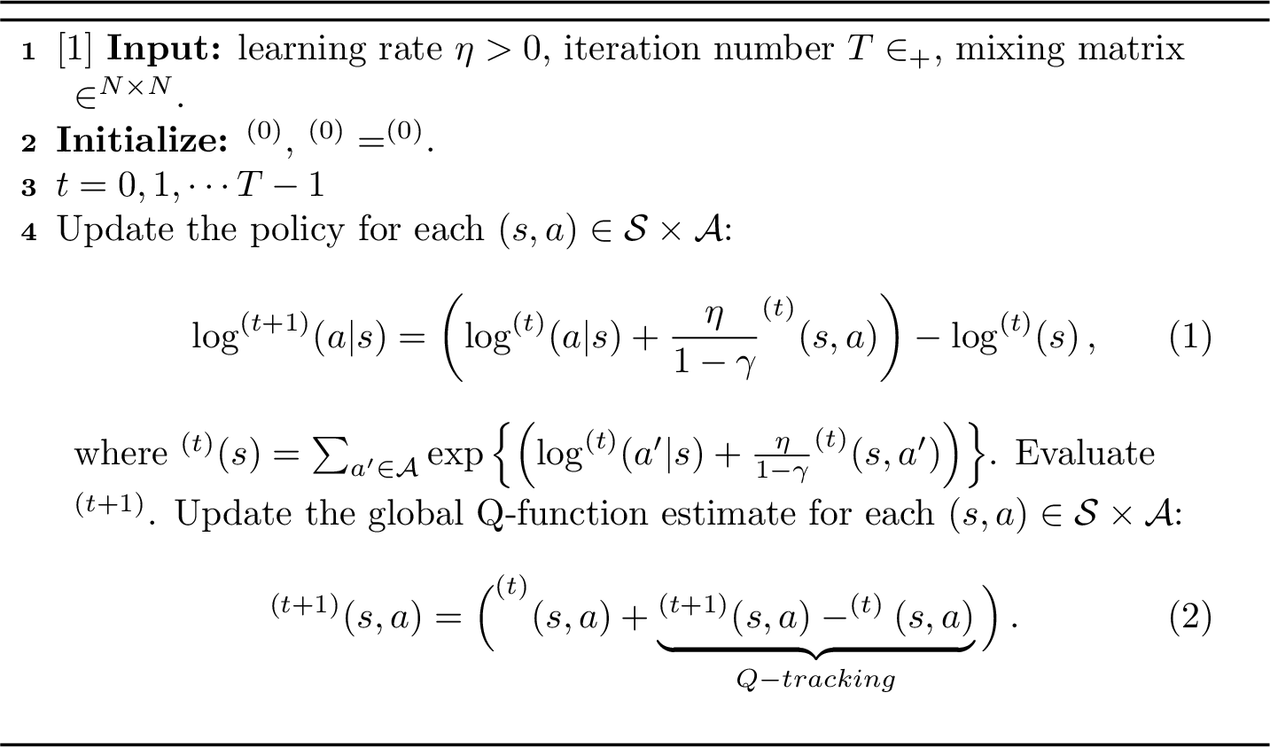
3.2.0.2 Entropy-regularized federated NPG methods.

Moving onto the entropy regularized case, we adopt similar algorithmic ideas to decentralize 14 , and propose the federated NPG (FedNPG) method with entropy regularization, summarized in Algorithm 2. Clearly, the entropy-regularized FedNPG method reduces to the vanilla FedNPG in the absence of the regularization (i.e., when \(\tau = 0\)).

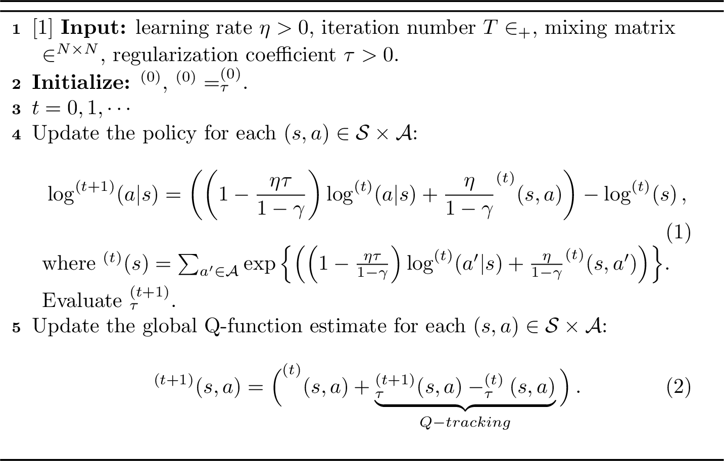
3.3 Global convergence of FedNPG↩︎

3.3.0.1 Convergence with exact policy evaluation.

We begin with the global convergence of FedNPG (cf. Algorithm 1), stated in the following theorem. The formal statement and proof of this result can be found in Appendix 6.3.

Theorem 1 characterizes the average-iterate convergence of the average policy \(\overline{\pi}^{(t)}\) (cf. 24 ) across the agents, which depends logarithmically on the size of the action space, and independently on the size of the state space. In addition, the consensus error of the local policies \(\pi_n^{(t)}\) towards the average policy \(\overline{\pi}^{(t)}\) is characterized in ?? . When \(T\geq \frac{128 \sqrt{N}\log |{\mathcal{A}}|\sigma^{4}}{(1-\sigma)^4}\), by optimizing the learning rate \(\eta=\left(\frac{(1-\gamma)^9(1-\sigma)^2 \log |{\mathcal{A}}|}{ 32 TN\sigma^2}\right)^{1/3}\) to balance the latter two terms, we arrive at \[\label{eq:convergence95rate95exact95opt95095inexact} \begin{align} \frac{1}{T}\sum_{t=0}^{T-1}\left(V^{\star}(\rho)-V^{\overline{\pi}^{(t)}}(\rho)\right) & \lesssim \frac{V^\star(d_\rho^{\pi^\star})}{(1-\gamma)T}+\frac{ N^{1/3}\sigma^{2/3}}{(1-\gamma)^3(1-\sigma)^{2/3}}\left(\frac{\log |{\mathcal{A}}|}{T}\right)^{2/3}\,. \\ \left\| \log\pi_n^{(t)}-\log\bar\pi^{(t)} \right\|_\infty & \lesssim \frac{ N^{2/3}\sigma^{1/3}}{(1-\gamma)(1-\sigma)^{1/3}}\left(\frac{\log |{\mathcal{A}}|}{T}\right)^{1/3}. \end{align}\tag{25}\] A few comments are in order.

• Server-client setting. When the network is fully connected, i.e., \(\sigma =0\), the convergence rate of FedNPG recovers the \(\mathcal{O}(1/T)\) rate, matching that of the centralized NPG established in [15].

• Well-connected networks. When the network is relatively well-connected in the sense of \(\frac{\sigma^2}{(1-\sigma)^2}\lesssim \frac{1-\gamma}{N^{1/2}}\), FedNPG first converges at the rate of \(\mathcal{O}(1/T)\), and then at the slower \(\mathcal{O}(1/T^{2/3})\) rate after \(T \gtrsim \frac{(1-\gamma)^3(1-\sigma)^2}{N\sigma^2}\).

• Poorly-connected networks. In addition, when the network is poorly connected in the sense of \(\frac{\sigma^2}{(1-\sigma)^2}\gtrsim \frac{1-\gamma}{N^{1/2}}\), we see that FedNPG converges at the slower \(\mathcal{O}(1/T^{2/3})\) rate.

We state the iteration complexity in Corollary 1.

3.3.0.2 Convergence with inexact policy evaluation.

In practice, the policies need to be evaluated using samples collected by the agents, where the Q-functions are only estimated approximately. We are interested in gauging how the approximation error impacts the performance of FedNPG, as demonstrated in the following theorem.

The formal statement and proof of this result is given in Appendix 6.4.

As long as \(\max_{n\in[N], t\in[T]}\big\| Q_{n}^{\pi_n^{(t)}}-q_{n}^{\pi_n^{(t)}}\big\|_\infty\leq \frac{\varepsilon}{C_3}\), inexact FedNPG reaches \(\frac{1}{T}\sum_{t=0}^{T-1}\big(V^{\star}(\rho)-V^{\overline{\pi}^{(t)}}(\rho)\big)\leq 2\varepsilon\) at the same iteration complexity as predicted in Corollary 1. Equipped with existing sample complexity bounds on policy evaluation, e.g. using a simulator as in [63] and [64], this immediate leads to a sample complexity bound for a federated actor-critic type algorithm for multi-task RL. We detail this in the following remark.

3.4 Global convergence of FedNPG with entropy regularization↩︎

3.4.0.1 Convergence with exact policy evaluation.

Next, we present our global convergence guarantee of entropy-regularized FedNPG with exact policy evaluation (cf. Algorithm 2).

The exact expressions of \(C_1\) and \(\eta_0\) are specified in Appendix 6.1. Theorem 3 confirms that entropy-regularized FedNPG converges at a linear rate to the optimal regularized policy, which is almost independent of the size of the state-action space, highlighting the positive role of entropy regularization in federated policy optimization. When the network is fully connected, i.e. \(\sigma =0\), the iteration complexity of entropy-regularized FedNPG reduces to \(\mathcal{O}\Big( \frac{1}{\eta\tau}\log\frac{1}{\varepsilon}\Big)\), matching that of the centralized entropy-regularized NPG established in [16]. When the network is less connected, one needs to be more conservative in the choice of learning rates, leading to a higher iteration complexity, as described in the following corollary.

3.4.0.2 Convergence with inexact policy evaluation.

Last but not the least, we present the informal convergence results of entropy-regularized FedNPG with inexact policy evaluation, whose formal version can be found in Appendix 6.2.

4 Federated NAC methods for multi-task RL↩︎

In this section, motivated by the design and analysis of FedNPG, we go beyond the tabular setting and exact policy evaluation, by proposing a federated natural actor-critic (FedNAC) method with function approximation and stochastic policy evaluation. Specifically, we consider the policy with function approximation under softmax parameterization of the following form: \[\label{eq:param95fa} f_\xi(a|s)=\frac{\exp(\phi^\top(s,a){\boldsymbol{\xi}})}{\sum_{a'\in{\mathcal{A}}}\exp(\phi^\top(s,a'){\boldsymbol{\xi}})},\tag{26}\] for all \((s,a)\in{\mathcal{S}}\times{\mathcal{A}}\) and \({\boldsymbol{\xi}}\in\mathbb{R}^p\), where \(\phi: {\mathcal{S}}\times{\mathcal{A}}\rightarrow \mathbb{R}^p\) is a known feature map. We assume \(\phi\) is bounded over \({\mathcal{S}}\times{\mathcal{A}}\), i.e., there exists \(C_\phi>0\) such that \[\left\| \phi(s,a) \right\|_2\leq C_\phi\] holds for all \((s,a)\in{\mathcal{S}}\times{\mathcal{A}}\). Following  [15], [38], given any \({\boldsymbol{w}}\in\mathbb{R}^p\), \(Q:{\mathcal{S}}\times{\mathcal{A}}\rightarrow \mathbb{R}\) and probability distribution \(\zeta\in\Delta({\mathcal{S}}\times{\mathcal{A}})\) over the state-action space, we define the function approximation error \(\ell({\boldsymbol{w}},Q,\zeta)\) as follows: \[\label{eq:l} \ell({\boldsymbol{w}},Q,\zeta)\mathrel{\vcenter{:}}= \mathbb{E}_{(s,a)\sim \zeta}\left[\left({\boldsymbol{w}}^\top\phi(s,a)-Q(s,a)\right)^2\right].\tag{27}\] By searching for \({\boldsymbol{w}}\) that minimizes \(\ell({\boldsymbol{w}},Q,\zeta)\), it approximates \(Q(s,a)\) using the feature map \(\phi\) with respect to the distribution \(\zeta\).

4.1 Algorithm design↩︎

Our proposed federated NAC method FedNAC could be seen as a decentralized version of Q-NPG method [15], [38], which we briefly review as follows.

4.1.0.1 Q-NPG method.

Q-NPG is a sample version of NPG with function approximation which is suitable for the case where \({\mathcal{S}}\) or \({\mathcal{A}}\) is large or infinite. We consider the policy with function approximation under softmax parameterization 26 .

Given an approximate solution \({\boldsymbol{w}}^{(t)}\) for minimizing the function approximation error \(\ell({\boldsymbol{w}},Q^{f_{\xi^{(t)}}},\tilde{d}_\nu^{f_{\xi^{(t)}}})\) (see 27 ), the Q-NPG update rule \({\boldsymbol{\xi}}^{(t+1)}={\boldsymbol{\xi}}^{(t)}+\alpha {\boldsymbol{w}}^{(t)}\), when plugged in parameterization 26 , results in the following policy update rule when we set \(\alpha=\eta/(1-\gamma)\): \[\label{eq:Q95NPG95policy95update} f^{(t+1)}(a|s)\propto f^{(t)}(a|s)\exp\left(\frac{\eta\phi^\top(s,a){\boldsymbol{w}}^{(t)}}{1-\gamma}\right)\,,\tag{30}\] which could be seen as the function approximation version of the update rule 13 of vanilla NPG method.

4.1.0.2 Federated NAC method.

Let us now discuss the high-level design of FedNAC, which is presented in Algorithm [alg:actor95critic]. At the \(t\)-th iteration (\(t =0,\ldots,T-1\)), denote the actor (concerning the policies) parameters of all agents as \({\boldsymbol{\xi}}^{(t)} =( {\boldsymbol{\xi}}_1^{(t)}, \ldots, {\boldsymbol{\xi}}_N^{(t)} )^{\top}\in \mathbb{R}^{N\times p}\), and the critic parameters of all agents as \({\boldsymbol{w}}^{(t)} =( {\boldsymbol{w}}_1^{(t)}, \ldots, {\boldsymbol{w}}_N^{(t)} )^{\top}\in \mathbb{R}^{N\times p}\) (concerning the local Q-values) and \({\boldsymbol{h}}^{(t)} =( {\boldsymbol{h}}_1^{(t)}, \ldots, {\boldsymbol{h}}_N^{(t)} )^{\top}\in \mathbb{R}^{N\times p}\) (concerning the global Q-values).

• First, the critic parameter \({\boldsymbol{w}}_n^{(t)}\) is locally updated at each agent by aiming to minimize \(\ell({\boldsymbol{w}},Q_n^{(t)}, \tilde{d}_{n}^{(t)})\) (cf. 27 ) with gradient descent, where \(Q_n^{(t)}\) is the local Q-function of the local policy \(f_{\xi_n^{(t)}}\), and \(\tilde{d}_n^{(t)}\) is the state-action visitation distribution induced by the local policy \(f_{\xi_n^{(t)}}\) and an initial state-action distribution \(\nu\) (determined from the data sampling mechanism, cf. 10 ). However, since \(Q_n^{(t)}\) is not directly available, it needs to be estimated from samples. Therefore, the critic update takes \(K\) steps of stochastic gradient descent with critic learning rate \(\beta\), given by \[\widetilde{{\boldsymbol{w}}}_{k+1}=\widetilde{{\boldsymbol{w}}}_k-\beta \big(\widetilde{{\boldsymbol{w}}}_k^\top \phi(s_k,a_k)-\widehat{Q}_{\xi}(s_k,a_k)\big)\phi(s_k,a_k),\] for \(k=0,\ldots, K-1\), where \((s_k, a_k)\) is sampled on the local policy \(f_{\xi_n^{(t)}}\), and \(\widehat{Q}_{\xi}(s_k,a_k)\) is a careful estimate of the Q-value using a trajectory with expected length \(1/(1-\gamma)\) (see Algorithm 4 adopted from [38]), and \(\widetilde{{\boldsymbol{w}}}_{0} = \boldsymbol{0}\) for simplicity. As a consequence, in line 4 of Algorithm 3, we have \[\label{eq:unbias95gd} \mathbb{E}\left[\widehat{\nabla}_w \ell(\widetilde{{\boldsymbol{w}}}_k,\widehat{Q}^\pi,\tilde{d}^{f_\xi})\right]=\nabla_w \ell(\widetilde{{\boldsymbol{w}}}_k,\widehat{Q}^\pi,\tilde{d}^{f_\xi})\,.\tag{31}\] The final critic is updated as \({\boldsymbol{w}}_n^{(t)} = \frac{1}{K}\sum_{k=1}^K \widetilde{{\boldsymbol{w}}}_k\). The total sample complexity of the critic update per iteration is then on the order of \(K/(1-\gamma)\).

• Next, the critic parameter \({\boldsymbol{h}}_n^{(t)}\) for estimating the global Q-function can then be estimated by averaging with the neighbors with the Q-tracking term, given by \({\boldsymbol{h}}^{(t)}={\boldsymbol{W}}\left({\boldsymbol{h}}^{(t-1)}+{\boldsymbol{w}}^{(t)}-{\boldsymbol{w}}^{(t-1)}\right).\)

• Finally, the actor parameter \({\boldsymbol{\xi}}_n^{(t)}\) can be updated via averaging with the neighbors along with the policy gradient informed by \({\boldsymbol{h}}_n^{(t)}\), given by \({\boldsymbol{\xi}}^{(t+1)}={\boldsymbol{W}}\left({\boldsymbol{\xi}}^{(t)}+\alpha {\boldsymbol{h}}^{(t)}\right),\) where \(\alpha\) is the learning rate of the actor.

Note that the sample complexity of FedNAC is on the order of \(KT/(1-\gamma)\). An important aspect of the FedNAC method is that the policy is updated using trajectory data collected via executing the learned policy, which is closer to practice and more challenging to learn than using the generative model.

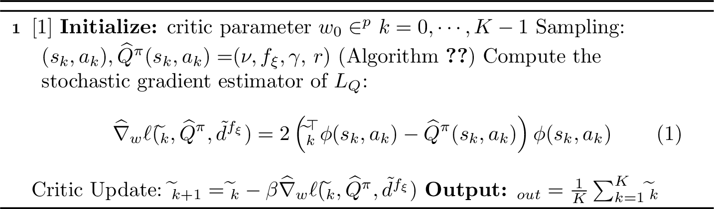
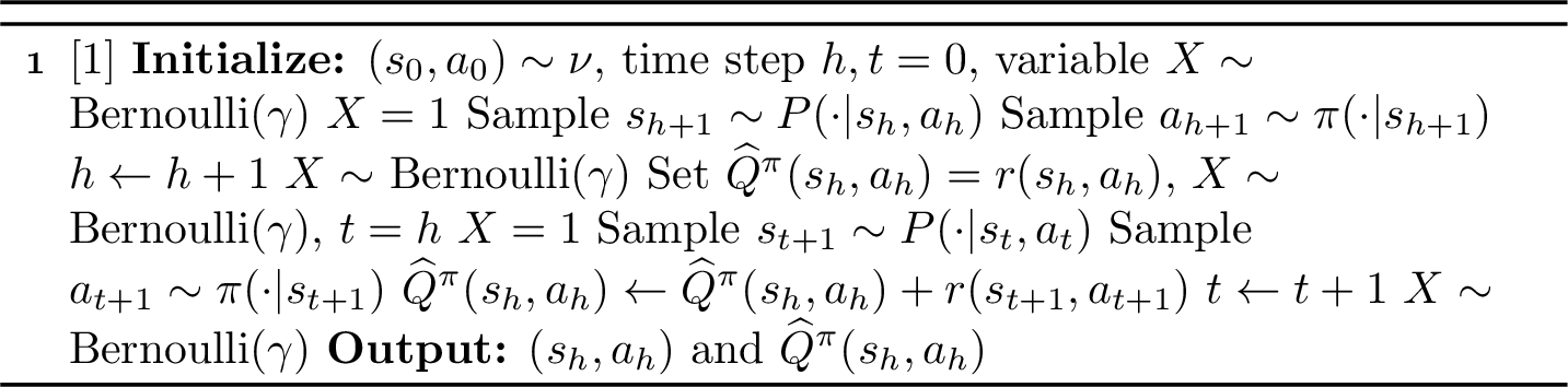
4.2 Theoretical guarantees↩︎

We first state the assumptions that are needed to guarantee the convergence of Algorithm [alg:actor95critic], which are all commonly used in the literature, e.g., [15], [38]. To begin, we require the covariance matrix of the feature map induced by the initial state-action distribution \(\nu\) satisfies the following assumption to guarantee the convergence of the critic.

We also need to ensure that the Q-values can be well approximated by the linear function approximation using feature map \(\phi(s,a)\), which is captured next.

We denote the average approximation error as \(\bar\varepsilon_{\text{approx}}=\frac{1}{N}\sum_{n=1}^N\varepsilon_{\text{approx}}^n\). Similar as [38], we need the following assumption that bounds the transfer errors due to distribution shifts.

Note that if we choose \(\nu(s,a)>0\) for all \((s,a)\in{\mathcal{S}}\times{\mathcal{A}}\), then Assumption 4 is guaranteed to hold true (see Lemma 7 in Appendix 7). We are now ready to state the convergence guarantee, whose formal version and proof could be found in Appendix 7.

In the server-client setting when \(\sigma=0\), to reach ?? , it suffices to choose \(T=\mathcal{O}\left(\frac{1}{(1-\gamma)\varepsilon}\right)\) and \(K=\mathcal{O}\left(\frac{1}{(1-\gamma)^6\varepsilon^2}\right)\), leading to a total sample complexity of \(KT/(1-\gamma) = \mathcal{O}\left(\frac{1}{(1-\gamma)^8\varepsilon^3}\right)\) per agent, and \(T=\mathcal{O}\left(\frac{1}{(1-\gamma)\varepsilon}\right)\) rounds of communication. The sample complexity matches that of (centralized) Q-NPG established in [38] with a single agent. On the other end, in the fully decentralized setting when \(\sigma\) is not close to 0, FedNAC requires \(\mathcal{O}\left(\frac{1}{(1-\gamma)^{45/4}\varepsilon^{7/2}(1-\sigma)^{3/2}}\right)\) samples for each agent and \(\mathcal{O}\left(\frac{1}{\varepsilon^{3/2}(1-\gamma)^{17/4}(1-\sigma)^{3/2}}\right)\) rounds of communication to reach ?? , for sufficiently small \(\varepsilon\). Encouragingly, the dependency on the accuracy level \(\varepsilon\) — the dominating factor — in the sample complexity matches that of FedNPG given in ?? when assuming access to the generative model, which allows query of arbitrary state-action pairs. In contrast, FedNAC only collects on-policy samples, and therefore is much more challenging to guarantee its convergence.

5 Conclusions↩︎

This work proposes the first provably efficient federated NPG (FedNPG) methods for solving vanilla and entropy-regularized multi-task RL problems in the fully decentralized setting. The established finite-time global convergence guarantees are almost independent of the size of the state-action space up to some logarithmic factor, and illuminate the impacts of the size and connectivity of the network. Furthermore, the proposed FedNPG methods are provably robust vis-a-vis inexactness of local policy evaluations. Last but not least, we also propose FedNAC, which can be viewed as an extension of FedNPG with function approximation and stochastic policy evaluation, and establish its finite-time sample complexity. Future directions include generalizing the framework of federated policy optimization to allow personalized policy learning in a shared environment.

Acknowledgments↩︎

The work of T. Yang, S. Cen and Y. Chi are supported in part by the grants ONR N00014-19-1-2404, NSF CCF-1901199, CCF-2106778, AFRL FA8750-20-2-0504, and a CMU Cylab seed grant. The work of Y. Wei is supported in part by the the NSF grants DMS-2147546/2015447, CAREER award DMS-2143215, CCF-2106778, and the Google Research Scholar Award. The work of Y. Chen is supported in part by the Alfred P. Sloan Research Fellowship, the Google Research Scholar Award, the AFOSR grant FA9550-22-1-0198, the ONR grant N00014-22-1-2354, and the NSF grants CCF-2221009 and CCF-1907661. S. Cen is also gratefully supported by Wei Shen and Xuehong Zhang Presidential Fellowship, Boeing Scholarship, and JP Morgan Chase PhD Fellowship.

6 Convergence analysis of FedNPG↩︎

For technical convenience, we present first the analysis for entropy-regularized FedNPG and then for vanilla FedNPG.

6.1 Analysis of entropy-regularized FedNPG with exact policy evaluation↩︎

To facilitate analysis, we introduce several notation below. For all \(t\geq 0\), we recall \(\overline{\pi}^{(t)}\) as the normalized geometric mean of \(\{\pi_n^{(t)}\}_{n\in[N]}\): \[\label{eq:overline95pi} \overline{\pi}^{(t)}\mathrel{\vcenter{:}}= \mathrm{softmax}\left(\frac{1}{N}\sum_{n=1}^N \log \pi_n^{(t)}\right)\,,\tag{32}\] from which we can easily see that for each \((s,a)\in \mathcal{S}\times \mathcal{A}\), \(\overline{\pi}^{(t)}(a|s)\propto \left(\prod_{n=1}^N \pi_n^{(t)}(a|s)\right)^{\frac{1}{N}}\). We denote the soft \(Q\)-functions of \(\overline{\pi}^{(t)}\) by \(\overline{{\boldsymbol{Q}}}_\tau^{(t)}\): \[\label{eq:overline95Q95tau95t95vec} \overline{{\boldsymbol{Q}}}_\tau^{(t)}\mathrel{\vcenter{:}}= \begin{pmatrix} Q_{\tau,1}^{\overline{\pi}^{(t)}}\\ \vdots\\ Q_{\tau,N}^{\overline{\pi}^{(t)}}\end{pmatrix}\,.\tag{33}\]

In addition, we define \(\widehat{Q}_\tau^{(t)}\), \(\overline{Q}_\tau^{(t)}\in \mathbb{R}^{|\mathcal{S}||\mathcal{A}|}\) and \(\overline{V}_\tau^{(t)}\in \mathbb{R}^{|\mathcal{S}|}\) as follows \[\tag{34} \begin{align} \widehat{Q}_\tau^{(t)}&\mathrel{\vcenter{:}}=\frac{1}{N}\sum_{n=1}^N Q_{\tau,n}^{\pi_n^{(t)}}\,, \tag{35}\\ \overline{Q}_\tau^{(t)}&\mathrel{\vcenter{:}}= Q_\tau^{\overline{\pi}^{(t)}}=\frac{1}{N}\sum_{n=1}^N Q_{\tau,n}^{\overline{\pi}^{(t)}}\,. \tag{36}\\ \overline{V}_\tau^{(t)}&\mathrel{\vcenter{:}}= V_\tau^{\overline{\pi}^{(t)}}=\frac{1}{N}\sum_{n=1}^N V_{\tau,n}^{\overline{\pi}^{(t)}}\,.\tag{37} \end{align}\] For notational convenience, we also denote \[\label{eq:alpha} \alpha\mathrel{\vcenter{:}}= 1-\frac{\eta\tau}{1-\gamma}\,.\tag{38}\]

Following [61], we introduce the following auxiliary sequence \(\{{\boldsymbol{\xi}}^{(t)}=(\xi_1^{(t)},\cdots,\xi_N^{(t)})^\top\in\mathbb{R}^{N\times|\mathcal{S}||\mathcal{A}|}\}_{t=0,1,\cdots}\), each recursively defined as \[\tag{39} \begin{align} \forall (s,a)\in \mathcal{S}\times \mathcal{A}:\quad{\boldsymbol{\xi}}^{(0)}(s,a)&\mathrel{\vcenter{:}}= \frac{\left\| \exp \left(Q_\tau^\star(s,\cdot)/\tau\right) \right\|_1}{\left\| \exp \left(\frac{1}{N}\sum_{n=1}^N\log\pi_n^{(0)}(\cdot|s)\right) \right\|_1}\cdot {\boldsymbol{\pi}}^{(0)}(a|s)\,, \tag{40}\\ \log{\boldsymbol{\xi}}^{(t+1)}(s,a)&={\boldsymbol{W}}\left(\alpha\log{\boldsymbol{\xi}}^{(t)}(s,a)+(1-\alpha){\boldsymbol{T}}^{(t)}(s,a)/\tau\right)\,,\tag{41} \end{align}\] where \({\boldsymbol{T}}^{(t)}(s,a)\) is updated via [eq:Q95tracking950]. Similarly, we introduce an averaged auxiliary sequence \(\{\overline{\xi}^{(t)}\in\mathbb{R}^{|\mathcal{S}||\mathcal{A}|}\}\) given by \[\tag{42} \begin{align} \forall (s,a)\in \mathcal{S}\times \mathcal{A}:\quad \overline{\xi}^{(0)}(s,a)&\mathrel{\vcenter{:}}= \left\| \exp \left(Q_\tau^\star(s,\cdot)/\tau\right) \right\|_1\cdot \overline{\pi}^{(0)}(a|s)\,,\\ \log\overline{\xi}^{(t+1)}(s,a)&= \alpha\log\overline{\xi}^{(t)}(s,a)+(1-\alpha)\widehat{Q}_\tau^{(t)}(s,a)/\tau. \tag{43} \end{align}\]

We introduces four error metrics defined as \[\begin{align} \Omega_1^{(t)}&\mathrel{\vcenter{:}}=\big\| u^{(t)} \big\|_\infty\,,\tag{44}\\ \Omega_2^{(t)}&\mathrel{\vcenter{:}}=\big\| v^{(t)} \big\|_\infty\,,\tag{45}\\ \Omega_3^{(t)}&\mathrel{\vcenter{:}}=\big\| Q_\tau^\star -\tau \log \overline{\xi}^{(t)} \big\|_\infty\,,\tag{46}\\ \Omega_4^{(t)}&\mathrel{\vcenter{:}}=\max\left\{0, -\min_{s,a}\left(\overline{Q}_\tau^{(t)}(s,a)-\tau\log\overline{\xi}^{(t)}(s,a)\right)\right\},\tag{47} \end{align}\] where \(u^{(t)},v^{(t)}\in\mathbb{R}^{|{\mathcal{S}}||{\mathcal{A}}|}\) are defined as \[\begin{align} u^{(t)}(s,a)&\mathrel{\vcenter{:}}= \big\| \log{\boldsymbol{\xi}}^{(t)}(s,a)-\log\overline{\xi}^{(t)}(s,a){\boldsymbol{1}}_N \big\|_2\,,\tag{48}\\ v^{(t)}(s,a)&\mathrel{\vcenter{:}}= \big\| {\boldsymbol{T}}^{(t)}(s,a)-\widehat{Q}_\tau^{(t)}(s,a){\boldsymbol{1}}_N \big\|_2\,.\tag{49} \end{align}\] We collect the error metrics above in a vector \(\mathbf{\Omega}^{(t)}\in\mathbb{R}^4\): \[\label{eq:Omega} \mathbf{\Omega}^{(t)}\mathrel{\vcenter{:}}=\left(\Omega_1^{(t)},\Omega_2^{(t)}, \Omega_3^{(t)}, \Omega_4^{(t)}\right)^\top\,.\tag{50}\]

With the above preparation, we are ready to state the convergence guarantee of Algorithm 2 in Theorem 6 below, which is the formal version of Theorem 3.

The dependency of \(\eta_0\) on \(N,\gamma,\tau,\sigma,|{\mathcal{A}}|\) is made clear in Lemma 2 that will be presented momentarily in this section. The rest of this section is dedicated to the proof of Theorem 6. We first state a key lemma that tracks the error recursion of Algorithm 2.

Let \(\rho(\eta)\) denote the spectral norm of \({\boldsymbol{A}}(\eta)\). As \(\mathbf{\Omega}^{(t)} \geq 0\), it is immediate from ?? that \[\big\| \mathbf{\Omega}^{(t)} \big\|_2\leq \rho(\eta)^t\big\| \mathbf{\Omega}^{(0)} \big\|_2\,,\] and therefore we have \[\left\| \overline{Q}_\tau^{(t)}-Q_\tau^\star \right\|_\infty\leq 2\gamma\big\| \mathbf{\Omega}^{(t)} \big\|_\infty \leq 2\gamma \rho(\eta)^t\big\| \mathbf{\Omega}^{(0)} \big\|_2\,,\] and \[\big\| \log\overline{\pi}^{(t)}-\log\pi_\tau^\star \big\|_\infty\leq \frac{2}{\tau}\big\| \mathbf{\Omega}^{(t)} \big\|_\infty \leq \frac{2}{\tau} \rho(\eta)^t\big\| \mathbf{\Omega}^{(0)} \big\|_2\,.\] It remains to bound the spectral radius \(\rho(\eta)\), which is achieved by the following lemma.

6.2 Analysis of entropy-regularized FedNPG with inexact policy evaluation↩︎

We define the collection of inexact Q-function estimates as \[\begin{align} {\boldsymbol{q}}_\tau^{(t)} \mathrel{\vcenter{:}}= \Big( q_{\tau,1}^{\pi_1^{(t)}},\cdots, q_{\tau,N}^{\pi_N^{(t)}}\Big)^\top, \end{align}\] and then the update rule [eq:Q95tracking] should be understood as \[\label{eq:Q95tracking95inexact} {\boldsymbol{T}}^{(t+1)}(s,a)={\boldsymbol{W}}\left({\boldsymbol{T}}^{(t)}(s,a)+{\boldsymbol{q}}_\tau^{(t+1)}(s,a)-{\boldsymbol{q}}_\tau^{(t)}(s,a) \right)\tag{51}\] in the inexact setting. For notational simplicity, we define \(e_n\in\mathbb{R}\) as \[\label{eq:delta95n} e_n:= \max_{t\in[T]}\left\| Q_{\tau,n}^{\pi_n^{(t)}}-q_{\tau,n}^{\pi_n^{(t)}} \right\|_\infty\,,\quad n\in[N]\,,\tag{52}\] and let \({\boldsymbol{e}}=(e_1,\cdots,e_n)^\top\). Define \(\widehat{q}_\tau^{(t)}\), the approximation of \(\widehat{Q}_\tau^{(t)}\) as \[\begin{align} \widehat{q}_\tau^{(t)}&\mathrel{\vcenter{:}}=\frac{1}{N}\sum_{n=1}^N q_{\tau,n}^{\pi_n^{(t)}}\,. \label{eq:hat95q95tau95t} \end{align}\tag{53}\]

With slight abuse of notation, we adapt the auxiliary sequence \(\{\overline{\xi}^{(t)}\}_{t=0,\cdots}\) to the inexact updates as \[\begin{align} \overline{\xi}^{(0)}(s,a)&\mathrel{\vcenter{:}}= \left\| \exp \left(Q_\tau^\star(s,\cdot)/\tau\right) \right\|_1\cdot \overline{\pi}^{(0)}(a|s)\,, \tag{54}\\ \overline{\xi}^{(t+1)}(s,a)&\mathrel{\vcenter{:}}= \left[\overline{\xi}^{(t)}(s,a)\right]^\alpha \exp\left((1-\alpha)\frac{\widehat{q}_\tau^{(t)}(s,a)}{\tau}\right)\,,\quad \forall (s,a)\in \mathcal{S}\times \mathcal{A}, \,\,t\geq 0\,.\tag{55} \end{align}\] In addition, we define \[\begin{align} \Omega_{1}^{(t)}&\mathrel{\vcenter{:}}=\left\| u^{(t)} \right\|_\infty\,,\tag{56}\\ \Omega_{2}^{(t)}&\mathrel{\vcenter{:}}=\left\| v^{(t)} \right\|_\infty\,,\tag{57}\\ \Omega_{3}^{(t)}&\mathrel{\vcenter{:}}=\left\| Q_\tau^\star -\tau \log \overline{\xi}^{(t)} \right\|_\infty\,,\tag{58}\\ \Omega_{4}^{(t)}&\mathrel{\vcenter{:}}=\max\left\{0, -\min_{s,a}\left(\overline{q}_\tau^{(t)}(s,a)-\tau\log\overline{\xi}^{(t)}(s,a)\right)\right\}\,,\tag{59} \end{align}\] where \[\begin{align} u^{(t)}(s,a)&\mathrel{\vcenter{:}}= \left\| \log{\boldsymbol{\xi}}^{(t)}(s,a)-\log\overline{\xi}^{(t)}(s,a){\boldsymbol{1}}_N \right\|_2\,,\tag{60}\\ v^{(t)}(s,a)&\mathrel{\vcenter{:}}= \left\| {\boldsymbol{T}}^{(t)}(s,a)-\widehat{q}_\tau^{(t)}(s,a){\boldsymbol{1}}_N \right\|_2\,.\tag{61} \end{align}\] We let \(\mathbf{\Omega}^{(t)}\) be \[\label{eq:Omega95inexact} \mathbf{\Omega}^{(t)}\mathrel{\vcenter{:}}=\left(\Omega_{1}^{(t)},\Omega_{2}^{(t)}, \Omega_{3}^{(t)}, \Omega_{4}^{(t)}\right)^\top\,.\tag{62}\]

With the above preparation, we are ready to state the inexact convergence guarantee of Algorithm 2 in Theorem 7 below, which is the formal version of Theorem 4.

From Theorem 7, we can conclude that if \[\label{eq:error95bound95E-DNPG} \max_{n\in[N],t\in[T]}\left\| Q_{\tau,n}^{\pi_n^{(t)}}-q_{\tau,n}^{\pi_n^{(t)}} \right\|_\infty\leq \frac{(1-\gamma)(1-\rho(\eta))\varepsilon}{2\gamma\left(\sigma\sqrt{N}(2(1-\gamma)+M\sqrt{N}\eta)+2\gamma^2+\eta\tau\right)}\,,\tag{63}\] then inexact entropy-regularized FedNPG could still achieve 2\(\varepsilon\)-accuracy (i.e. \(\left\| \overline{Q}_\tau^{(t)}-Q_\tau^\star \right\|_\infty\leq 2\varepsilon\)) within \(\max\left\{\frac{2}{\tau\eta},\frac{4}{1-\sigma}\right\}\log\frac{2\gamma \left\| \mathbf{\Omega}^{(0)} \right\|_2}{\varepsilon}\) iterations.

The rest of this section outlines the proof of Theorem 7. We first state a key lemma that tracks the error recursion of Algorithm 2 with inexact policy evaluation, which is a modified version of Lemma 1.

By ?? , we have \[\forall t\in N_+:\quad \mathbf{\Omega}^{(t)}\leq{\boldsymbol{A}}(\eta)^t \mathbf{\Omega}^{(0)}+\sum_{s=1}^t{\boldsymbol{A}}(\eta)^{t-s}{\boldsymbol{b}}(\eta)\,,\] which gives \[\begin{align} \left\| \mathbf{\Omega}^{(t)} \right\|_2 &\leq \rho(\eta)^t\left\| \mathbf{\Omega}^{(0)} \right\|_2+\sum_{s=1}^t\rho(\eta)^{t-s}\left\| {\boldsymbol{b}}(\eta) \right\|_2 \left\| {\boldsymbol{e}} \right\|_\infty \notag\\ & \leq \rho(\eta)^t\left\| \mathbf{\Omega}^{(0)} \right\|_2+ \frac{\sigma\sqrt{N}(2(1-\gamma)+M\sqrt{N}\eta)+2\gamma^2+\eta\tau}{(1-\gamma)(1-\rho(\eta))}\left\| {\boldsymbol{e}} \right\|_\infty\,.\label{eq:estimate95t95inexact} \end{align}\tag{64}\] Here, 64 follows from \(\left\| {\boldsymbol{b}}(\eta) \right\|_2\leq \left\| {\boldsymbol{b}}(\eta) \right\|_1=\frac{\sigma\sqrt{N}(2(1-\gamma)+M\sqrt{N}\eta)+2\gamma^2+\eta\tau}{1-\gamma}\left\| {\boldsymbol{e}} \right\|_\infty\) and \(\sum_{s=1}^t\rho(\eta)^{t-s}\leq 1/(1-\rho(\eta))\). Recall that the bound on \(\rho(\eta)\) has already been established in Lemma 2. Therefore we complete the proof of Theorem 7 by combining the above inequality with ?? and ?? in a similar fashion as before. We omit further details for conciseness.

6.3 Analysis of FedNPG with exact policy evaluation↩︎

We state the formal version of Theorem 1 below.

The rest of this section is dedicated to prove Theorem 8. Similar to 33 , we denote the \(Q\)-functions of \(\overline{\pi}^{(t)}\) by \(\overline{{\boldsymbol{Q}}}^{(t)}\): \[\label{eq:overline95Q95t95vec} \overline{{\boldsymbol{Q}}}^{(t)}\mathrel{\vcenter{:}}= \begin{pmatrix} Q_{1}^{\overline{\pi}^{(t)}}\\ \vdots\\ Q_{N}^{\overline{\pi}^{(t)}}\end{pmatrix}\,.\tag{65}\]

In addition, similar to 34 , we define \(\widehat{Q}^{(t)}\), \(\overline{Q}^{(t)}\in \mathbb{R}^{|\mathcal{S}||\mathcal{A}|}\) and \(\overline{V}^{(t)}\in \mathbb{R}^{|\mathcal{S}|}\) as follows \[\tag{66} \begin{align} \widehat{Q}^{(t)}&\mathrel{\vcenter{:}}=\frac{1}{N}\sum_{n=1}^N Q_{n}^{\pi_n^{(t)}}\,, \tag{67}\\ \overline{Q}^{(t)}&\mathrel{\vcenter{:}}= Q^{\overline{\pi}^{(t)}}=\frac{1}{N}\sum_{n=1}^N Q_{n}^{\overline{\pi}^{(t)}}\,. \tag{68}\\ \overline{V}^{(t)}&\mathrel{\vcenter{:}}= V^{\overline{\pi}^{(t)}}=\frac{1}{N}\sum_{n=1}^N V_{n}^{\overline{\pi}^{(t)}}\,.\tag{69} \end{align}\]

Following the same strategy in the analysis of entropy-regularized FedNPG, we introduce the auxiliary sequence \(\{{\boldsymbol{\xi}}^{(t)}=(\xi_1^{(t)},\cdots,\xi_N^{(t)})^\top\in\mathbb{R}^{N\times|\mathcal{S}||\mathcal{A}|}\}\) recursively: \[\begin{align} {\boldsymbol{\xi}}^{(0)}(s,a)&\mathrel{\vcenter{:}}= \frac{1}{\left\| \exp \left(\frac{1}{N}\sum_{n=1}^N\log\pi_n^{(0)}(\cdot|s)\right) \right\|_1}\cdot {\boldsymbol{\pi}}^{(0)}(a|s)\,, \tag{70}\\ \log{\boldsymbol{\xi}}^{(t+1)}(s,a)&={\boldsymbol{W}}\left(\log{\boldsymbol{\xi}}^{(t)}(s,a)+\frac{\eta}{1-\gamma}{\boldsymbol{T}}^{(t)}(s,a)\right),\tag{71} \end{align}\] as well as the averaged auxiliary sequence \(\{\overline{\xi}^{(t)}\in\mathbb{R}^{|\mathcal{S}||\mathcal{A}|}\}\): \[\begin{align} \overline{\xi}^{(0)}(s,a)&\mathrel{\vcenter{:}}= \overline{\pi}^{(0)}(a|s)\,, \tag{72}\\ \log\overline{\xi}^{(t+1)}(s,a)&\mathrel{\vcenter{:}}= \log\overline{\xi}^{(t)}(s,a) + \frac{\eta}{1-\gamma}\widehat{Q}^{(t)}(s,a)\,,\quad \forall (s,a)\in \mathcal{S}\times \mathcal{A}, \,\,t\geq 0\,.\tag{73} \end{align}\] As usual, we collect the consensus errors in a vector \(\mathbf{\Omega}^{(t)} = (\big\| u^{(t)} \big\|_\infty,\big\| v^{(t)} \big\|_\infty)^\top\), where \(u^{(t)},v^{(t)}\in \mathbb{R}^{|{\mathcal{S}}||{\mathcal{A}}|}\) are defined as: \[\begin{align} u^{(t)}(s,a)& \mathrel{\vcenter{:}}= \big\| \log {\boldsymbol{\xi}}^{(t)}(s,a)-\log\overline{\xi}^{(t)}(s,a){\boldsymbol{1}}_N \big\|_2\,,\tag{74}\\ v^{(t)}(s,a)& \mathrel{\vcenter{:}}= \big\| {\boldsymbol{T}}^{(t)}(s,a)-\widehat{Q}^{(t)}(s,a){\boldsymbol{1}}_N \big\|_2\,.\tag{75} \end{align}\]

6.3.0.1 Step 1: establishing the error recursion.

The next key lemma establishes the error recursion of Algorithm 1.

Note that when all \(\pi_n^{(0)}\) in Algorithm 1 are initialized as uniform distribution, \(\mathbf{\Omega}^{(0)}={\boldsymbol{0}}\) and ?? indicates ?? in Theorem 8.

6.3.0.2 Step 2: bounding the value functions.

Let \({\boldsymbol{p}}\in\mathbb{R}^2\) be defined as: \[\label{eq:p} {\boldsymbol{p}}(\eta)= \begin{pmatrix} p_1(\eta)\\ p_2(\eta) \end{pmatrix} \mathrel{\vcenter{:}}= \frac{2(1+\gamma)\gamma}{(1-\gamma)^4} \begin{pmatrix} \frac{\sigma(1-\gamma)\left(1-\sigma-(1+\gamma)\gamma\sqrt{N}\sigma\eta/(1-\gamma)^3\right)\eta}{(1-\gamma)\left(1-\sigma-(1+\gamma)\gamma\sqrt{N}\sigma^2\eta/(1-\gamma)^3\right)(1-\sigma)-J\sigma^2\eta}\\ \frac{\sigma\eta^2}{(1-\gamma)\left(1-\sigma-(1+\gamma)\gamma\sqrt{N}\sigma^2\eta/(1-\gamma)^3\right)(1-\sigma)-J\sigma^2\eta} \end{pmatrix};\tag{76}\] the rationale for this choice will be made clear momentarily. We define the following Lyapunov function \[\label{eq:Lyapunov} \Phi^{(t)}(\eta)=\phi^{(t)}(\eta)+{\boldsymbol{p}}(\eta)^\top \mathbf{\Omega}^{(t)}\,,\quad \forall t\geq 0\,,\tag{77}\] which satisfies \[\begin{align} \Phi^{(t+1)}(\eta)&=\phi^{(t+1)}(\eta)+{\boldsymbol{p}}(\eta)^\top \mathbf{\Omega}^{(t+1)}\notag\\ &\leq \phi^{(t)}(\eta)+\frac{2(1+\gamma)\gamma}{(1-\gamma)^4}\eta\big\| u^{(t)} \big\|_\infty-\eta\left(V^{\star}(\rho)-\overline{V}^{(t)}(\rho)\right) + {\boldsymbol{p}}(\eta)^\top\left({\boldsymbol{B}}(\eta)\mathbf{\Omega}^{(t)}+{\boldsymbol{d}}(\eta)\right) \notag \\ &= \Phi^{(t)}(\eta)+\left[{\boldsymbol{p}}(\eta)^\top\left({\boldsymbol{B}}(\eta)-{\boldsymbol{I}}\right)+\left(\frac{2(1+\gamma)\gamma}{(1-\gamma)^4}\eta, 0\right)\right]\mathbf{\Omega}^{(t)}-\eta\left(V^{\star}(\rho)-\overline{V}^{(t)}(\rho)\right)\notag\\ &\qquad +p_2(\eta)\frac{(1+\gamma)\gamma N\sigma}{(1-\gamma)^4}\eta\,.\label{eq:ineq95lyap} \end{align}\tag{78}\] Here, the second inequality follows from ?? . One can verify that the second term vanishes due to the choice of \({\boldsymbol{p}}(\eta)\): \[\label{eq:magic} {\boldsymbol{p}}(\eta)^\top\left({\boldsymbol{B}}(\eta)-{\boldsymbol{I}}\right)+\left(\frac{2(1+\gamma)\gamma}{(1-\gamma)^4}\eta, 0\right)=(0,0)\,.\tag{79}\] Therefore, we conclude that \[V^{\star}(\rho)-\overline{V}^{(t)}(\rho)\leq\frac{\Phi^{(t)}(\eta)-\Phi^{(t+1)}(\eta)}{\eta}+p_2(\eta)\frac{(1+\gamma)\gamma N\sigma}{(1-\gamma)^4}\,.\] Averaging over \(t = 0,\cdots, T-1\), \[\begin{align} &\frac{1}{T}\sum_{t=0}^{T-1}\left(V^{\star}(\rho)-\overline{V}^{(t)}(\rho)\right)\notag\\ &\leq \frac{\Phi^{(0)}(\eta)-\Phi^{(T)}(\eta)}{\eta T}+\frac{2(1+\gamma)^2\gamma^2}{(1-\gamma)^8}\cdot\frac{N\sigma^2\eta^2 }{(1-\gamma)(1-\sigma-(1+\gamma)\gamma\sqrt{N}\sigma^2\eta/(1-\gamma)^3)(1-\sigma)-\sigma ^2 J\eta}\,.\label{eq:ub95to95be95refined} \end{align}\tag{80}\]

6.3.0.3 Step 3: simplifying the expression.

We first upper bound the first term in the RHS of 80 . Assuming uniform initialization for all \(\pi_n^{(0)}\) in Algorithm 1, we have \(\left\| u^{(0)} \right\|_\infty=\left\| v^{(0)} \right\|_\infty=0\), and \[\mathbb{E}_{s\sim d_\rho^{\pi^\star}}\left[\mathsf{KL}\big({{\pi^\star(\cdot|s)}\,\|\,{\overline{\pi}^{(0)}(\cdot|s)}}\big)\right]\leq\log|{\mathcal{A}}|.\] Therefore, putting together relations 77 and ?? we have \[\begin{align} \frac{\Phi^{(0)}(\eta)-\Phi^{(T)}(\eta)}{\eta T} & \leq \frac{\log |{\mathcal{A}}|}{T\eta}+\frac{1}{T}\left({\boldsymbol{p}}(\eta)^\top\mathbf{\Omega}^{(0)}/\eta+\frac{V^\star(d_\rho^{\pi^\star})}{1-\gamma}\right)=\frac{\log |{\mathcal{A}}|}{T\eta}+\frac{V^\star (d_\rho^{\pi^\star})}{T(1-\gamma)}\,,\label{eq:ub95term1} \end{align}\tag{81}\]

To continue, we upper bound the second term in the RHS of 80 . Note that \[\eta\leq \eta_1\leq \frac{(1-\sigma)(1-\gamma)^3}{2(1+\gamma)\gamma\sqrt{N}\sigma^2}\,,\] which gives \[\label{eq:bd95denominator951} \frac{(1+\gamma)\gamma\sqrt{N}\sigma^2}{(1-\gamma)^3}\eta\leq \frac{1-\sigma}{2}.\tag{82}\]

Thus we have\[\begin{align} &(1-\gamma)(1-\sigma-(1+\gamma)\gamma\sqrt{N}\sigma^2\eta/(1-\gamma)^3)(1-\sigma)-J\sigma^2\eta\notag\\ & \geq (1-\gamma)(1-\sigma)^2/2-J\sigma^2\eta_1\notag\\ & \geq (1-\gamma)(1-\sigma)^2/4\,,\label{eq:lb95denominator} \end{align}\tag{83}\] where the first inequality follows from 82 and the second inequality follows from the definition of \(\eta_1\) and \(J\). By 83 , we deduce \[\label{eq:ub95term2} \frac{2(1+\gamma)^2\gamma^2}{(1-\gamma)^8}\cdot\frac{N\sigma^2\eta^2}{(1-\gamma)(1-\sigma-(1+\gamma)\gamma\sqrt{N}\sigma^2\eta/(1-\gamma)^3)(1-\sigma)-J\sigma^2\eta}\leq \frac{8(1+\gamma)^2\gamma^2 N\sigma^2}{(1-\gamma)^9(1-\sigma)^2}\eta^2\,,\tag{84}\] and our advertised bound ?? thus follows from plugging 81 and 84 into 80 .

6.4 Analysis of FedNPG with inexact policy evaluation↩︎

We state the formal version of Theorem 2 below.

We next outline the proof of Theorem 9. With slight abuse of notation, we again define \(e_n\in\mathbb{R}\) as \[\label{eq:delta95n95vanilla} e_n:= \max_{t\in[T]}\left\| Q_{n}^{\pi_n^{(t)}}-q_{n}^{\pi_n^{(t)}} \right\|_\infty\,,\quad n\in[N]\,,\tag{85}\] and let \({\boldsymbol{e}}=(e_1,\cdots,e_n)^\top\). We define the collection of inexact Q-function estimates as \[\begin{align} {\boldsymbol{q}}^{(t)} \mathrel{\vcenter{:}}= \Big( q_{1}^{\pi_1^{(t)}},\cdots, q_{N}^{\pi_N^{(t)}}\Big)^\top, \end{align}\] and then the update rule [eq:Q95tracking950] should be understood as \[\label{eq:Q95tracking95095inexact} {\boldsymbol{T}}^{(t+1)}(s,a)={\boldsymbol{W}}\left({\boldsymbol{T}}^{(t)}(s,a)+{\boldsymbol{q}}^{(t+1)}(s,a)-{\boldsymbol{q}}^{(t)}(s,a) \right)\tag{86}\] in the inexact setting. Define \(\widehat{q}^{(t)}\), the approximation of \(\widehat{Q}^{(t)}\) as \[\begin{align} \widehat{q}^{(t)}&\mathrel{\vcenter{:}}=\frac{1}{N}\sum_{n=1}^N q_{n}^{\pi_n^{(t)}}\,, \label{eq:hat95q95t} \end{align}\tag{87}\] we adapt the averaged auxiliary sequence \(\{\overline{\xi}^{(t)}\in\mathbb{R}^{|\mathcal{S}||\mathcal{A}|}\}\) to the inexact updates as follows: \[\begin{align} \overline{\xi}^{(0)}(s,a)&\mathrel{\vcenter{:}}= \overline{\pi}^{(0)}(a|s)\,, \tag{88}\\ \overline{\xi}^{(t+1)}(s,a)&\mathrel{\vcenter{:}}= \overline{\xi}^{(t)}(s,a)\exp\left(\frac{\eta}{1-\gamma}\widehat{q}^{(t)}(s,a)\right)\,,\quad \forall (s,a)\in \mathcal{S}\times \mathcal{A}, \,\,t\geq 0\,.\tag{89} \end{align}\]

As usual, we define the consensus error vector as \(\mathbf{\Omega}^{(t)} = (\big\| u^{(t)} \big\|_\infty,\big\| v^{(t)} \big\|_\infty)^\top\), where \(u^{(t)},v^{(t)}\in \mathbb{R}^{|{\mathcal{S}}||{\mathcal{A}}|}\) are given by \[\begin{align} u^{(t)}(s,a)\mathrel{\vcenter{:}}= & \left\| \log{\boldsymbol{\xi}}^{(t)}(s,a)-\log\overline{\xi}^{(t)}(s,a){\boldsymbol{1}}_N \right\|_2\,,\tag{90}\\ v^{(t)}(s,a)\mathrel{\vcenter{:}}= & \left\| {\boldsymbol{T}}^{(t)}(s,a)-\widehat{q}^{(t)}(s,a){\boldsymbol{1}}_N \right\|_2\,.\tag{91} \end{align}\] The following lemma characterizes the dynamics of the error vector \(\mathbf{\Omega}^{(t)}\), perturbed by additional approximation error.

Similar to 78 , we can recursively bound \(\Phi^{(t)}(\eta)\) (defined in 77 ) as \[\begin{align} \Phi^{(t+1)}(\eta)&=\phi^{(t+1)}(\eta)+{\boldsymbol{p}}(\eta)^\top \mathbf{\Omega}^{(t+1)}\notag\\ & \overset{\eqref{eq:A095inexact}}{\leq} \phi^{(t)}(\eta)+\frac{2(1+\gamma)\gamma}{(1-\gamma)^4}\eta\left\| u^{(t)} \right\|_\infty+\frac{2\eta}{(1-\gamma)^2}\left\| {\boldsymbol{e}} \right\|_\infty-\eta\left(V^{\star}(\rho)-\overline{V}^{(t)}(\rho)\right) \nonumber \\ &\qquad\qquad +{\boldsymbol{p}}(\eta)^\top\left({\boldsymbol{B}}(\eta)\mathbf{\Omega}^{(t)}+{\boldsymbol{d}}(\eta)+{\boldsymbol{c}}(\eta)\right) \nonumber \\ &= \Phi^{(t)}(\eta)+\underbrace{\left[{\boldsymbol{p}}(\eta)^\top\left({\boldsymbol{B}}(\eta)-{\boldsymbol{I}}\right)+\left(\frac{2(1+\gamma)\gamma}{(1-\gamma)^4}\eta, 0\right)\right]}_{ = (0,0)~\sf{via~}\eqref{eq:magic} }\mathbf{\Omega}^{(t)}-\eta\left(V^{\star}(\rho)-\overline{V}^{(t)}(\rho)\right)\notag\\ &\qquad\qquad +p_2(\eta)\frac{(1+\gamma)\gamma N\sigma}{(1-\gamma)^4}\eta + \left[p_2(\eta)\sqrt{N}\sigma\left(\frac{(1+\gamma)\gamma \eta \sqrt{N}}{(1-\gamma)^3}+2\right)+\frac{2\eta}{(1-\gamma)^2}\right]\left\| {\boldsymbol{e}} \right\|_\infty\,. \label{eq:ineq95lyap95inexact} \end{align}\tag{92}\] From the above expression we know that \[V^{\star}(\rho)-\overline{V}^{(t)}(\rho)\leq\frac{\Phi^{(t)}(\eta)-\Phi^{(t+1)}(\eta)}{\eta}+p_2(\eta)\frac{(1+\gamma)\gamma N\sigma}{(1-\gamma)^4}+\left[p_2(\eta)\sqrt{N}\sigma\left(\frac{(1+\gamma)\gamma\sqrt{N}}{(1-\gamma)^3}+\frac{2}{\eta}\right)+\frac{2}{(1-\gamma)^2}\right]\left\| {\boldsymbol{e}} \right\|_\infty\,,\] which gives \[\begin{align} \frac{1}{T}\sum_{t=0}^{T-1}\left(V^{\star}(\rho)-\overline{V}^{(t)}(\rho)\right)&\leq \frac{\Phi^{(0)}(\eta)-\Phi^{(T)}(\eta)}{\eta T}+p_2(\eta)\frac{(1+\gamma)\gamma N\sigma}{(1-\gamma)^4}\notag\\ &\qquad +\left[p_2(\eta)\sqrt{N}\sigma\left(\frac{(1+\gamma)\gamma\sqrt{N}}{(1-\gamma)^3}+\frac{2}{\eta}\right)+\frac{2}{(1-\gamma)^2}\right]\left\| {\boldsymbol{e}} \right\|_\infty\,\label{eq:ub95to95be95refined95inexact} \end{align}\tag{93}\] via telescoping. Combining the above expression with 81 , 83 and 84 , we have \[\begin{align} \frac{1}{T}\sum_{t=0}^{T-1}\left(V^{\star}(\rho)-\overline{V}^{(t)}(\rho)\right) &\leq \frac{\log |{\mathcal{A}}|}{T\eta}+\frac{V^\star (d_\rho^{\pi^\star})}{T(1-\gamma)}+\frac{8(1+\gamma)^2\gamma^2 N\sigma}{(1-\gamma)^9(1-\sigma)^2}\eta^2\notag\\ &\qquad +\left[\frac{8(1+\gamma)\gamma}{(1-\gamma)^5(1-\sigma)^2}\sqrt{N}\sigma\eta\left(\frac{(1+\gamma)\gamma\eta\sqrt{N}}{(1-\gamma)^3}+2\right)+\frac{2}{(1-\gamma)^2}\right]\left\| {\boldsymbol{e}} \right\|_\infty\,,\label{eq:ub95inexact} \end{align}\tag{94}\] which establishes ?? .

7 Convergence analysis of FedNAC↩︎

Let \(\pi^\star\) be an optimal policy and does not need to belong to the log-linear policy class. Fix a state distribution \(\rho\in\Delta({\mathcal{S}})\) and a state-action distribution \(\nu\). To simplify the notation, we denote \(d^{\pi^\star}_\rho\) as \(d_\star\), \(d^{f_{\bar{\boldsymbol{\xi}}^{(t)}}}\) as \(d^{(t)}\), \(\tilde{d}_n^{(t)}\) as \(\tilde{d}_\nu^{f_{\xi_n^{(t)}}}\), and define \(d_n^{(t)}\) and \(\bar d_n^{(t)}\) analogously. We also let \(Q_n^{(t)}\) denote \(Q_n^{\xi_n^{(t)}}\).

Define \[\label{eq:vartheta95rho} \vartheta_\rho\mathrel{\vcenter{:}}=\frac{1}{1-\gamma}\left\| \frac{d_\star}{\rho} \right\|_\infty\geq \frac{1}{1-\gamma}\tag{95}\] and assume \(\vartheta_\rho<\infty\).

We also introduce a weighted KL divergence given by \[\label{eq:weighted95KL} D_\star^{(t)}\mathrel{\vcenter{:}}=\mathbb{E}_{s\sim d_\star}\left[\mathsf{KL}\big({{\pi^\star(\cdot|s)}\,\|\,{\pi^{(t)}(\cdot|s)}}\big)\right]\,,\tag{96}\] where \(\mathsf{KL}\big({{\cdot}\,\|\,{\cdot}}\big):\mathbb{R}^{|{\mathcal{A}}|}\times\mathbb{R}^{|{\mathcal{A}}|}\rightarrow\mathbb{R}\) is the Kullback-Leibler (KL) divergence: \[\label{eq:KL} \forall f,g\in \mathbb{R}^{|{\mathcal{A}}|}:\quad \mathsf{KL}\big({{f}\,\|\,{g}}\big)\mathrel{\vcenter{:}}=\sum_{a\in{\mathcal{A}}}f(a)\log\left(\frac{f(a)}{g(a)}\right)\,.\tag{97}\]

Given a state distribution \(\rho\) and an optimal policy \(\pi^\star\), we define a state-action measure \(\tilde{d}^\star\) as \[\label{eq:tilde95d95star} \tilde{d}^\star(s,a)\mathrel{\vcenter{:}}= d_\star(s)\cdot \text{Unif}_{\mathcal{A}}(a)=\frac{d_\star(s)}{|{\mathcal{A}}|}.\tag{98}\]

The following theorem guarantees that for any fixed policy \(\pi\) and state-action distribution \(\nu\in\Delta({\mathcal{S}}\times{\mathcal{A}})\), the Q-Sampler algorithm (cf. Algorithm 4) samples \((s,a)\) from \(\tilde{d}_\nu^\pi\) and gives an unbiased estimate \(\widehat Q^\pi(s,a)\) of \(Q^\pi(s,a)\), whose proof can be found in [38].

To present the convergence results of FedNAC, we further introduce the following notation, where \(t\in{\mathbb{N}}\) represents the iteration step in FedNAC: \[\begin{align} \hat{{\boldsymbol{w}}}^{(t)}&\mathrel{\vcenter{:}}= \frac{1}{N}\sum_{n=1}^{N}{\boldsymbol{w}}_n^{(t)}, \tag{99}\\ \bar{\boldsymbol{\xi}}^{(t)}&\mathrel{\vcenter{:}}= \frac{1}{N}\sum_{n=1}^N {\boldsymbol{\xi}}_n^{(t)} ,\tag{100}\\ \bar f^{(t)} &\mathrel{\vcenter{:}}= f_{\bar\xi^{(t)}},\tag{101}\\ f_n^{(t)}&\mathrel{\vcenter{:}}= f_{\xi_n^{(t)}},\tag{102}\\ {\boldsymbol{w}}_{\star,n}^{(t)}&\in\arg\min_{\boldsymbol{w}}\ell \left({\boldsymbol{w}}, Q_n^{(t)},\tilde{d}_n^{(t)}\right),\tag{103}\\ \hat{\boldsymbol{w}}_\star^{(t)} &\mathrel{\vcenter{:}}= \frac{1}{N}\sum_{n=1}^N {\boldsymbol{w}}_{\star,n}^{(t)}.\tag{104} \end{align}\] For convenience of narration, we introduce the following bounded statistical error assumption.

When solving the regression problem with sampling based approaches, we can expect \(\varepsilon_{\text{stat}}^n=\mathcal{O}(1/K)\), where \(K\) is the iteration number of Algorithm 3.

The proof of Theorem 10 is postponed to Appendix 7.2.

The following lemma provide a (very pessimistic) upper bound of \(C_\nu\) in Assumption 4.

We give some key lemmas which will be used in our proof of Theorem 5.

For each iteration step \(t\) in Algorithm [alg:actor95critic], we let \(\bar{\boldsymbol{\xi}}^{(t)}\mathrel{\vcenter{:}}= \frac{1}{N}\sum_{n=1}^N{\boldsymbol{\xi}}^{(t)}_n=\frac{1}{N}{\boldsymbol{\xi}}^{(t)\top}{\boldsymbol{1}}_N\). We define \[\begin{align} \Omega_1^{(t)}&\mathrel{\vcenter{:}}=\mathbb{E}\left\| {\boldsymbol{\xi}}^{(t)}-{\boldsymbol{1}}_N\overline{{\boldsymbol{\xi}}}^{(t)\top} \right\|_{\mathrm F}^2,\tag{105}\\ \Omega_2^{(t)}&\mathrel{\vcenter{:}}=\mathbb{E}\left\| {\boldsymbol{h}}^{(t)}-{\boldsymbol{1}}_N\hat{{\boldsymbol{w}}}^{(t)\top} \right\|_{\mathrm F}^2,\tag{106} \end{align}\]

We let \[\begin{align} \bar \varepsilon_{\text{stat}}\mathrel{\vcenter{:}}=& \frac{1}{N}\sum_{n=1}^N\varepsilon_{\text{stat}}^n\,,\tag{107}\\ \bar \varepsilon_{\text{approx}}\mathrel{\vcenter{:}}=& \frac{1}{N}\sum_{n=1}^N\varepsilon_{\text{approx}}^n\,,\tag{108} \end{align}\] and define \(\delta^{(t)}\mathrel{\vcenter{:}}= V^\star-\bar V^{(t)}(\rho)\), where \(\bar V^{(t)}\) is shorthand for \(V^{\bar f^{(t)}}\). We give the following performance improvement lemma.

Now we are ready to give the formal version of Theorem 5 and its proof.

7.1 Proof of Theorem 11↩︎

We suppose Assumptions 1, 5, 2, 3 and 4 holds. By Lemma 12 and nonnegativity of each entry of \({\boldsymbol{C}}\), \({\boldsymbol{s}}\) and \(\mathbf{\Omega}^{(t)}\) where \(t\in{\mathbb{N}}\), it’s easy to see that \[\label{eq:matrix95fnac95sqrt} \sqrt{\mathbf{\Omega}^{(t+1)}}\leq \sqrt{{\boldsymbol{C}}}\sqrt{\mathbf{\Omega}^{(t)}}+\sqrt{{\boldsymbol{s}}},\tag{109}\] where \(\sqrt{\cdot}\) is exerted element-wise.

In addition, taking expectation on both sides of ?? and using the act that \[\mathbb{E}\left[\sqrt{2\left(\bar\varepsilon_{\text{approx}}+\frac{L_Q^2}{N}\left\| {\boldsymbol{\xi}}^{(t)}-{\boldsymbol{1}}_N\bar{\boldsymbol{\xi}}^{(t)\top} \right\|_{\mathrm F}^2\right)}\right]\leq\sqrt{2\bar\varepsilon_{\text{approx}}}+\sqrt{\frac{2L_Q^2}{N}\Omega_1^{(t)}},\] we have \[\begin{align} \label{eq:improve952} \vartheta_\rho \mathbb{E}[\delta^{(t+1)}] + \frac{\mathbb{E}[D_\star^{(t+1)}]}{(1-\gamma)\alpha}&\leq\vartheta_\rho\mathbb{E}[\delta^{(t)}] +\frac{\mathbb{E}[D_\star^{(t)}]}{(1-\gamma)\alpha}-\mathbb{E}[\delta^{(t)}]\notag\\ &+\frac{2\sqrt{C_\nu}(\vartheta_\rho +1)}{1-\gamma}\left(\sqrt{\bar\varepsilon_{\text{stat}}}+\sqrt{2\bar\varepsilon_{\text{approx}}}+\sqrt{\frac{2L_Q^2}{N}\Omega_1^{(t)}}\right). \end{align}\tag{110}\]

We define the Lyapunov function \(\Phi^{(t)}\) as follows: \[\label{eq:Lya} \Phi^{(t)}\mathrel{\vcenter{:}}= \vartheta_\rho\mathbb{E}[\delta^{(t)}] +\frac{\mathbb{E}[D_\star^{(t)}]}{(1-\gamma)\alpha} + {\boldsymbol{q}}^\top\sqrt{\mathbf{\Omega}^{(t)}},\tag{111}\] where \[\label{eq:q} {\boldsymbol{q}}=\begin{pmatrix} q_1\\ q_2 \end{pmatrix} =\begin{pmatrix} \frac{2L_Q\sqrt{2C_\nu}(\vartheta_\rho +1)}{(1-\gamma)\sqrt{N}}\cdot\frac{1}{1-\sqrt{1+\zeta}\sigma-\sqrt{(1+1/\zeta)c_{21}}\sigma\alpha/(1-\sqrt{c_{22}})}\\ \frac{2L_Q\sqrt{2C_\nu}(\vartheta_\rho +1)}{(1-\gamma)\sqrt{N}}\cdot\frac{\sqrt{1+1/\zeta}\sigma\alpha}{(1-\sqrt{1+\zeta}\sigma)(1-\sqrt{c_{22}})-\sqrt{(1+1/\zeta)c_{21}}\sigma\alpha} \end{pmatrix}.\tag{112}\]

It’s straightforward to verify that when \(\zeta=\frac{1-\sigma^2}{2}\), we have the entries in \(\boldsymbol{C}\) (cf. ?? ) satisfies \[\begin{align} c_{11}&<\frac{1+\sigma^2}{2},\tag{113}\\ c_{12}&\leq\frac{3\sigma^2\alpha^2}{1-\sigma^2}.\tag{114} \end{align}\]

Moreover, from \(\alpha\leq \frac{\sqrt{(1-\gamma)\mu}(1-\sigma^2)}{12\sqrt{2}\sigma L_Q}\) we deduce \[\label{eq:a22} c_{22}\leq \frac{3+\sigma^2}{4},\tag{115}\] which gives \[\label{eq:1-sqrt95a22} 1-\sqrt{c_{22}}\geq 1-\sqrt{\frac{3+\sigma^2}{4}}\geq \frac{1-\sigma^2}{8},\tag{116}\]

Also note that \(\alpha\leq \frac{(1-\sigma^2)^3\sqrt{(1-\gamma)\mu}}{768\sqrt{6}\sigma^2 L_Q}\) yields \[\sqrt{(1+1/\zeta)c_{21}}\sigma\alpha\leq \frac{(1-\sqrt{1+\zeta}\sigma)(1-\sqrt{c_{22}})}{2}.\] which together with 116 and the fact \(1-\sqrt{1+\zeta}\sigma\geq \frac{1-\sigma^2}{4}\) indicates \(q_1,q_2>0\) and that \[\begin{align} q_1&\leq\frac{16\sqrt{2}L_Q\sqrt{C_\nu}(\vartheta_\rho+1)}{(1-\sigma^2)(1-\gamma)\sqrt{N}},\\ q_2&\leq\frac{128\sqrt{6}L_Q\sqrt{C_\nu}(\vartheta_\rho+1)\sigma\alpha}{(1-\sigma^2)^{5/2}(1-\gamma)\sqrt{N}}.\label{eq:q2} \end{align}\tag{117}\]

Thus by 109 and 110 we have \[\begin{align} \Phi^{(t+1)}&=\vartheta_\rho \mathbb{E}[\delta^{(t+1)}] + \frac{\mathbb{E}[D_\star^{(t+1)}]}{(1-\gamma)\alpha}+{\boldsymbol{q}}^\top\sqrt{\mathbf{\Omega}^{(t+1)}}\notag\\ &\leq\vartheta_\rho\mathbb{E}[\delta^{(t)}] +\frac{\mathbb{E}[D_\star^{(t)}]}{(1-\gamma)\alpha}-\mathbb{E}[\delta^{(t)}]+{\boldsymbol{q}}^\top\left(\sqrt{{\boldsymbol{C}}}\sqrt{\mathbf{\Omega}^{(t)}}+\sqrt{{\boldsymbol{s}}}\right)\notag\\ &\qquad+\frac{2\sqrt{C_\nu}(\vartheta_\rho +1)}{1-\gamma}\left(\sqrt{\bar\varepsilon_{\text{stat}}}+\sqrt{2\bar\varepsilon_{\text{approx}}}+\sqrt{\frac{2L_Q^2}{N}\Omega_1^{(t)}}\right)\notag\\ &=\Phi^{(t)}+\left(\underbrace{{\boldsymbol{q}}^\top (\sqrt{{\boldsymbol{C}}}-{\boldsymbol{I}})+\left(\frac{2L_Q\sqrt{2C_\nu}(\vartheta_\rho +1)}{(1-\gamma)\sqrt{N}},0\right)}_{=(0,0)}\right)\sqrt{\mathbf{\Omega}^{(t)}}\notag\\ &\qquad+\frac{2\sqrt{C_\nu}(\vartheta_\rho +1)}{1-\gamma}\left(\sqrt{\bar\varepsilon_{\text{stat}}}+\sqrt{2\bar\varepsilon_{\text{approx}}}\right)+q_2\sqrt{s_2}-\mathbb{E}[\delta^{(t)}], \end{align}\] which gives \[\mathbb{E}[\delta^{(t)}]\leq \Phi^{(t)}- \Phi^{(t+1)} +\frac{2\sqrt{C_\nu}(\vartheta_\rho +1)}{1-\gamma}\left(\sqrt{\bar\varepsilon_{\text{stat}}}+\sqrt{2\bar\varepsilon_{\text{approx}}}\right)+q_2\sqrt{s_2}.\] Summing the above inequality over \(t=0,1,\cdots,T-1\) and divide both sides by \(T\), we have \[\frac{1}{T}\sum_{t=0}^{T-1}\mathbb{E}[\delta^{(t)}]\leq \frac{\Phi^{(0)}-\Phi^{(t)}}{T}+\frac{2\sqrt{C_\nu}(\vartheta_\rho +1)}{1-\gamma}\left(\sqrt{\bar\varepsilon_{\text{stat}}}+\sqrt{2\bar\varepsilon_{\text{approx}}}\right)+q_2\sqrt{s_2}.\]

Since \[\label{eq:b2} s_2\leq \frac{18\sigma^2 N}{(1-\sigma^2)(1-\gamma)\mu}\left(\bar\varepsilon_{\text{stat}}+C_\nu \bar\varepsilon_{\text{approx}}\right)+\frac{72\sigma^2L_Q^2 N}{(1-\gamma)^3\mu^3(1-\sigma^2)}\left((1-\gamma)\mu\bar\varepsilon_{\text{stat}}+C_\phi^2\right)\alpha^2,\tag{118}\] and \[\label{eq:qhi0} \Phi^{(0)}-\Phi^{(t)}\leq\Phi^{(0)}\leq\frac{\vartheta_\rho}{1-\gamma}+\frac{\mathbb{E}[D_\star^{(0)}]}{(1-\gamma)\alpha}+\frac{16\sqrt{2}L_Q\sqrt{C_\nu}(\vartheta_\rho+1)}{(1-\sigma^2)(1-\gamma)\sqrt{N}}\left(\sqrt{\Omega_1^{(0)}}+\frac{8\sqrt{3}\sigma\alpha}{\sqrt{1-\sigma^2}}\sqrt{\Omega_2^{(0)}}\right),\tag{119}\] we have (recall that \(L_Q=\frac{2C_\phi\gamma(1+\gamma)}{(1-\gamma)^2}\leq\frac{4C_\phi}{(1-\gamma)^2}\)) \[\begin{align} &V^{\star}(\rho)-\frac{1}{T}\sum_{t=0}^{T-1}\mathbb{E}\left[\bar V^{(t)}(\rho)\right]\notag\\ &\leq \frac{D_\star^{(0)}+\alpha\vartheta_\rho}{T(1-\gamma)\alpha}+\frac{1}{T}\cdot \frac{64\sqrt{2}C_\phi\sqrt{C_\nu}(\vartheta_\rho+1)}{(1-\sigma^2)(1-\gamma)^3\sqrt{N}}\left(\sqrt{\Omega_1^{(0)}}+\frac{8\sqrt{3}\sigma\alpha}{\sqrt{1-\sigma^2}}\sqrt{\Omega_2^{(0)}}\right)\notag\\ &\quad+\left[\frac{2\sqrt{C_\nu}(\vartheta_\rho +1)}{1-\gamma}+\sqrt{\frac{18\sigma^2 N}{(1-\sigma^2)(1-\gamma)\mu}+\frac{1152\sigma^2 C_\phi^2 N\alpha^2}{(1-\gamma)^6\mu^2(1-\sigma^2)}}\cdot \frac{512\sqrt{6}C_\phi\sqrt{C_\nu}(\vartheta_\rho+1)\sigma\alpha}{(1-\sigma^2)^{5/2}(1-\gamma)^3\sqrt{N}}\right]\sqrt{\bar\varepsilon_{\text{stat}}}\notag\\ &\quad+\left[\frac{2\sqrt{2C_\nu}(\vartheta_\rho +1)}{1-\gamma}+\sqrt{\frac{18\sigma^2 NC_\nu}{(1-\sigma^2)(1-\gamma)\mu}}\cdot \frac{512\sqrt{6}C_\phi\sqrt{C_\nu}(\vartheta_\rho+1)\sigma\alpha}{(1-\sigma^2)^{5/2}(1-\gamma)^3\sqrt{N}}\right]\sqrt{\bar\varepsilon_{\text{approx}}}\notag\\ &\quad+\frac{6144\sqrt{2}\sigma^2\sqrt{C_\nu}(\vartheta_\rho+1)C_\phi^3\alpha^2}{(1-\gamma)^{13/2}\mu^{3/2}(1-\sigma^2)^3}.\label{eq:rate95pre} \end{align}\tag{120}\]

By Theorem 10 we know that \(\sqrt{\bar\varepsilon_{\text{stat}}}\) could be upper bounded as follows: \[\label{eq:bound95l95minimizer95eps95stat} \sqrt{\bar\varepsilon_{stat}}\leq\frac{2}{(1-\gamma)^2\sqrt{K}}\left((\sqrt{2p}+1)C_\phi^2+\sqrt{2p}\mu(1-\gamma)\right).\tag{121}\]

?? follows from plugging 121 into 120 and noting that when \({\boldsymbol{\xi}}_1^{(0)}=\cdots={\boldsymbol{\xi}}_N^{(0)}\), \(\Omega_1^{(0)}=0\).

7.1.0.1 Bounding the consensus errors.

Similar to Step 4 in Appendix 8.4, to bound the consensus error \(\left\| \log f_n^{(t)}-\log\bar f^{(t)} \right\|_\infty\) for all \(n\in[N]\), we first upper bound the eigenvalue of \(\rho({\boldsymbol{C}})\)—the spectral norm of \({\boldsymbol{C}}\).

The characteristic polynomial of \({\boldsymbol{C}}\) is \[\begin{align} f(\lambda)&=(\lambda-c_{11})(\lambda-c_{22})-c_{12}c_{21}\\ &=\lambda^2-(c_{11}+c_{22})\lambda+c_{11}c_{22}-c_{12}c_{21}\,, \end{align}\] which gives \[\begin{align} \rho({\boldsymbol{C}})&\leq\frac{c_{11}+c_{22}+\sqrt{(c_{11}+c_{22})^2-4(c_{11}c_{12}-c_{12}c_{21})}}{2}\notag\\ &=\frac{c_{11}+c_{22}+\sqrt{(c_{22}-c_{11})^2+4c_{12}c_{21}}}{2}\notag\\ &\leq\frac{c_{11}+c_{22}+c_{22}-c_{11}+2\sqrt{c_{12}c_{21}}}{2}\notag\\ &=c_{22}+\sqrt{c_{12}c_{21}}\notag\\ &\leq\frac{3+\sigma^2}{4}+\frac{\sqrt{3}\sigma\alpha}{\sqrt{1-\sigma^2}}\cdot\frac{12\sqrt{2}L_Q\sigma}{\sqrt{1-\sigma^2}(1-\gamma)\mu}\notag\\ &\leq\frac{3+\sigma^2}{4}+\frac{\sigma(1-\sigma^2)^2}{64}\notag\\ &\leq\frac{49+15\sigma^2}{64}<1\,,\label{eq:lambda40C41} \end{align}\tag{122}\] where the third inequality uses 114 , 115 , and the fourth inequality uses ?? .

Therefore, similar to 186 , when \(\alpha\leq\alpha_1\), we have \[\begin{align} \left\| \mathbf{\Omega}^{(t)} \right\|_2 &\leq\left(\frac{49}{64}\sigma+\frac{15}{64}\right)^t\left\| \mathbf{\Omega}^{(0)} \right\|_2+\frac{64s_2}{15(1-\sigma^2)}\,.\label{eq:consensus95error95pre95fnac} \end{align}\tag{123}\] Combining the above inequality with 118 , and 121 , we obtain ?? .

7.2 Proof of Theorem 10↩︎

The proof of Theorem 10 could be found in Appendix C.5 in [38]. We present it for completeness. To prove Theorem 10, we need the following Theorem 12.

In the proof of Theorem 10 we’ll show that for Algorithm 3, the assumptions in Theorem 12 are all satisfied and thus we can use the result ?? .

8 Proof of key lemmas for FedNPG↩︎

8.1 Proof of Lemma 1↩︎

Before proceeding, we summarize several useful properties of the auxiliary sequences (cf. 39 and 42 ), whose proof is postponed to Appendix 8.6.

8.1.0.1 Step 1: bound \(u^{(t+1)}(s,a)=\big\| \log{\boldsymbol{\xi}}^{(t+1)}(s,a)-\log\overline{\xi}^{(t+1)}(s,a){\boldsymbol{1}}_N \big\|_2\).

By 41 and 43 we have \[\begin{align} u^{(t+1)}(s,a)&=\big\| \log{\boldsymbol{\xi}}^{(t+1)}(s,a)-\log\overline{\xi}^{(t+1)}(s,a){\boldsymbol{1}}_N \big\|_2\notag\\ &=\left\| \alpha\Big({\boldsymbol{W}}\log{\boldsymbol{\xi}}^{(t)}(s,a)-\log\overline{\xi}^{(t)}(s,a){\boldsymbol{1}}_N\Big)+(1-\alpha)\Big({\boldsymbol{W}}{\boldsymbol{T}}^{(t)}(s,a)-\widehat{Q}_\tau^{(t)}(s,a){\boldsymbol{1}}_N\Big)/\tau \right\|_2\notag\\ &\leq\sigma\alpha\big\| \log{\boldsymbol{\xi}}^{(t)}(s,a)-\log\overline{\xi}^{(t)}(s,a){\boldsymbol{1}}_N \big\|_2+\frac{1-\alpha}{\tau}\sigma\big\| {\boldsymbol{T}}^{(t)}(s,a)-\widehat{Q}_\tau^{(t)}(s,a){\boldsymbol{1}}_N \big\|_2\notag\\ &\leq\sigma\alpha\big\| u^{(t)} \big\|_\infty+\frac{1-\alpha}{\tau}\sigma\big\| v^{(t)} \big\|_\infty,\label{eq:B} \end{align}\tag{127}\] where the penultimate step results from the averaging property of \({\boldsymbol{W}}\) (property 21 ). Taking maximum over \((s,a) \in {\mathcal{S}}\times{\mathcal{A}}\) establishes the bound on \(\Omega_1^{(t+1)}\) in ?? .

8.1.0.2 Step 2: bound \(v^{(t+1)}(s,a)=\big\| {\boldsymbol{T}}^{(t+1)}(s,a)-\widehat{Q}_\tau^{(t+1)}(s,a){\boldsymbol{1}}_N \big\|_2\).

By [eq:Q95tracking] we have \[\begin{align} &\big\| {\boldsymbol{T}}^{(t+1)}(s,a)-\widehat{Q}_\tau^{(t+1)}(s,a){\boldsymbol{1}}_N \big\|_2\notag\\ &=\left\| {\boldsymbol{W}}\left({\boldsymbol{T}}^{(t)}(s,a)+{\boldsymbol{Q}}_\tau^{(t+1)}(s,a)-{\boldsymbol{Q}}_\tau^{(t)}(s,a)\right)-\widehat{Q}_\tau^{(t+1)}(s,a){\boldsymbol{1}}_N \right\|_2\notag\\ &=\left\| \left({\boldsymbol{W}}{\boldsymbol{T}}^{(t)}(s,a)-\widehat{Q}_\tau^{(t)}(s,a){\boldsymbol{1}}_N\right)+{\boldsymbol{W}}\left({\boldsymbol{Q}}_\tau^{(t+1)}(s,a)-{\boldsymbol{Q}}_\tau^{(t)}(s,a)\right)+\left(\widehat{Q}_\tau^{(t)}(s,a)-\widehat{Q}_\tau^{(t+1)}(s,a)\right){\boldsymbol{1}}_N \right\|_2\notag\\ &\leq\sigma\big\| {\boldsymbol{T}}^{(t)}(s,a)-\widehat{Q}_\tau^{(t)}(s,a){\boldsymbol{1}}_N \big\|_2+\sigma\left\| \left({\boldsymbol{Q}}_\tau^{(t+1)}(s,a)-{\boldsymbol{Q}}_\tau^{(t)}(s,a)\right)+\left(\widehat{Q}_\tau^{(t)}(s,a)-\widehat{Q}_\tau^{(t+1)}(s,a)\right){\boldsymbol{1}}_N \right\|_2\notag\\ &\leq\sigma\big\| {\boldsymbol{T}}^{(t)}(s,a)-\widehat{Q}_\tau^{(t)}(s,a){\boldsymbol{1}}_N \big\|_2+\sigma\big\| {\boldsymbol{Q}}_\tau^{(t+1)}(s,a)-{\boldsymbol{Q}}_\tau^{(t)}(s,a) \big\|_2\,,\label{eq:diff95T95Q} \end{align}\tag{128}\] where the penultimate step uses property 21 , and the last step is due to \[\begin{align} &\left\| \left({\boldsymbol{Q}}_\tau^{(t+1)}(s,a)-{\boldsymbol{Q}}_\tau^{(t)}(s,a)\right)+\left(\widehat{Q}_\tau^{(t)}(s,a)-\widehat{Q}_\tau^{(t+1)}(s,a)\right){\boldsymbol{1}}_N \right\|_2^2\\ &=\big\| {\boldsymbol{Q}}_\tau^{(t+1)}(s,a)-{\boldsymbol{Q}}_\tau^{(t)}(s,a) \big\|_2^2+N\big(\widehat{Q}_\tau^{(t)}(s,a)-\widehat{Q}_\tau^{(t+1)}(s,a)\big)^2\\ &\qquad -2\sum_{n=1}^N\left(Q_{\tau,n}^{\pi_n^{(t+1)}}(s,a)-Q_{\tau,n}^{\pi_n^{(t)}}(s,a)\right)\left(\widehat{Q}_\tau^{(t+1)}(s,a)-\widehat{Q}_\tau^{(t)}(s,a)\right)\\ &=\big\| {\boldsymbol{Q}}_\tau^{(t+1)}(s,a)-{\boldsymbol{Q}}_\tau^{(t)}(s,a) \big\|_2^2-N\big(\widehat{Q}_\tau^{(t)}(s,a)-\widehat{Q}_\tau^{(t+1)}(s,a)\big)^2\\ &\leq \big\| {\boldsymbol{Q}}_\tau^{(t+1)}(s,a)-{\boldsymbol{Q}}_\tau^{(t)}(s,a) \big\|_2^2\,. \end{align}\]

8.1.0.3 Step 3: bound \(\big\| Q_\tau^\star -\tau \log \overline{\xi}^{(t+1)} \big\|_\infty\).

We decompose the term of interest as \[\begin{align} Q_\tau^\star -\tau \log \overline{\xi}^{(t+1)}&=Q_\tau^\star -\tau\alpha \log \overline{\xi}^{(t)} - (1-\alpha)\widehat{Q}_\tau^{(t)}\notag\\ &=\alpha(Q_\tau^\star -\tau \log \overline{\xi}^{(t)})+(1-\alpha)(Q_\tau^\star-\overline{Q}_\tau^{(t)})+(1-\alpha)(\overline{Q}_\tau^{(t)}-\widehat{Q}_\tau^{(t)}), \end{align}\] which gives \[\label{eq:pre95A} \big\| Q_\tau^\star -\tau \log \overline{\xi}^{(t+1)} \big\|_\infty\leq \alpha\big\| Q_\tau^\star -\tau \log \overline{\xi}^{(t)} \big\|_\infty+(1-\alpha)\big\| Q_\tau^\star-\overline{Q}_\tau^{(t)} \big\|_\infty+(1-\alpha)\big\| \overline{Q}_\tau^{(t)}-\widehat{Q}_\tau^{(t)} \big\|_\infty\,.\tag{129}\] Note that we can upper bound \(\big\| \overline{Q}_\tau^{(t)}-\widehat{Q}_\tau^{(t)} \big\|_\infty\) by \[\begin{align} \big\| \overline{Q}_\tau^{(t)} -\widehat{Q}_\tau^{(t)} \big\|_\infty &= \left\| \frac{1}{N}\sum_{n=1}^N Q_{\tau,n}^{\pi_n^{(t)}}-\frac{1}{N}\sum_{n=1}^N Q_{\tau,n}^{\overline{\pi}^{(t)}} \right\|_\infty \notag\\ &\leq\frac{1}{N}\sum_{n=1}^N\big\| Q_{\tau,n}^{\pi_n^{(t)}} - Q_{\tau,n}^{\overline{\pi}^{(t)}} \big\|_\infty\notag\\ &\leq \frac{M}{N}\sum_{n=1}^N \big\| \log\xi_n^{(t)}-\log\overline{\xi}^{(t)} \big\|_\infty {\leqslant}M\big\| u^{(t)} \big\|_\infty.\label{eq:diff95Q95tau95overline} \end{align}\tag{130}\] The last step is due to \(\big|\log\xi_n^{(t)}(s,a)-\log\overline{\xi}^{(t)}(s,a)\big|\leq u^{(t)}(s,a)\), while the penultimate step results from writing \[\begin{align} \overline{\pi}^{(t)}(\cdot|s)&=\mathrm{softmax}\left({\log\overline{\xi}^{(t)}(s,\cdot)}\right)\,,\\ \pi_n^{(t)}(\cdot|s)&=\mathrm{softmax}\left({\log\xi_n^{(t)}(s,\cdot)}\right)\,, \end{align}\] and applying the following lemma.

Plugging 130 into 129 gives \[\label{eq:A} \big\| Q_\tau^\star -\tau \log \overline{\xi}^{(t+1)} \big\|_\infty\leq \alpha\big\| Q_\tau^\star -\tau \log \overline{\xi}^{(t)} \big\|_\infty+(1-\alpha)\big\| Q_\tau^\star-\overline{Q}_\tau^{(t)} \big\|_\infty+(1-\alpha)M\big\| u^{(t)} \big\|_\infty\,.\tag{131}\]

8.1.0.4 Step 4: bound \(\big\| {\boldsymbol{Q}}_\tau^{(t+1)}(s,a)-{\boldsymbol{Q}}_\tau^{(t)}(s,a) \big\|_2\).

Let \(w^{(t)}:{\mathcal{S}}\times{\mathcal{A}}\rightarrow\mathbb{R}\) be defined as \[\label{eq:r} \forall (s,a)\in{\mathcal{S}}\times{\mathcal{A}}:\quad w^{(t)}(s,a)\mathrel{\vcenter{:}}=\big\| \log{\boldsymbol{\xi}}^{(t+1)}(s,a)-\log{\boldsymbol{\xi}}^{(t)}(s,a)-(1-\alpha)V_\tau^\star(s){\boldsymbol{1}}_N/\tau \big\|_2\,.\tag{132}\] Again, we treat \(w^{(t)}\) as vectors in \(\mathbb{R}^{|{\mathcal{S}}||{\mathcal{A}}|}\) whenever it is clear from context. For any \((s,a)\in{\mathcal{S}}\times{\mathcal{A}}\) and \(n\in[N]\), by Lemma 15 it follows that \[\begin{align} \left|Q_{\tau,n}^{\pi_n^{(t+1)}}(s,a)-Q_{\tau,n}^{\pi_n^{(t)}}(s,a)\right| & \leq M\max_{s\in{\mathcal{S}}}\big\| \log\xi_n^{(t+1)}(s,\cdot)-\log\xi_n^{(t)}(s,\cdot)-(1-\alpha)V_\tau^\star(s){\boldsymbol{1}}_{|{\mathcal{A}}|}/\tau \big\|_\infty\notag\\ & \leq M \max_{s\in{\mathcal{S}}} \max_{a\in{\mathcal{A}}}w^{(t)}(s,a) \leq M \big\| w^{(t)} \big\|_\infty\,,\label{eq:Q95to95pi} \end{align}\tag{133}\] and consequently \[\label{eq:bound95by95r953} \big\| {\boldsymbol{Q}}_\tau^{(t+1)}(s,a)-{\boldsymbol{Q}}_\tau^{(t)}(s,a) \big\|_2\leq M\sqrt{N}\big\| w^{(t)} \big\|_\infty\,.\tag{134}\] It boils down to control \(\left\| w^{(t)} \right\|_\infty\). To do so, we first note that for each \((s,a)\in{\mathcal{S}}\times{\mathcal{A}}\), we have \[\begin{align} &w^{(t)}(s,a)\notag\\ &=\big\| {\boldsymbol{W}}\left(\alpha\log{\boldsymbol{\xi}}^{(t)}(s,a)+(1-\alpha){\boldsymbol{T}}^{(t)}(s,a)/\tau\right)-\log{\boldsymbol{\xi}}^{(t)}(s,a)-(1-\alpha)V_\tau^\star(s){\boldsymbol{1}}_N/\tau \big\|_2\notag\\ &\overset{(a)}{=}\left\| \alpha({\boldsymbol{W}}-{\boldsymbol{I}}_N)\left(\log{\boldsymbol{\xi}}^{(t)}(s,a)-\log\overline{\xi}^{(t)}(s,a){\boldsymbol{1}}_N\right)+(1-\alpha)\left({\boldsymbol{W}}{\boldsymbol{T}}^{(t)}(s,a)/\tau-\log{\boldsymbol{\xi}}^{(t)}(s,a)-V_\tau^\star(s){\boldsymbol{1}}_N/\tau\right) \right\|_2\notag\\ &\overset{(b)}{\leq} 2\alpha \big\| \log{\boldsymbol{\xi}}^{(t)}(s,a)-\log\overline{\xi}^{(t)}(s,a){\boldsymbol{1}}_N \big\|_2+\frac{1-\alpha}{\tau}\big\| {\boldsymbol{W}}{\boldsymbol{T}}^{(t)}(s,a)-\tau\log{\boldsymbol{\xi}}^{(t)}(s,a)-V_\tau^\star(s){\boldsymbol{1}}_N \big\|_2\label{eq:bound95w} \end{align}\tag{135}\] where (a) is due to the doubly stochasticity property of \({\boldsymbol{W}}\) and (b) is from the fact \(\|{\boldsymbol{W}}-{\boldsymbol{I}}_N\|_2 \leq 2\). We further bound the second term as follows: \[\begin{align} &\left\| {\boldsymbol{W}}{\boldsymbol{T}}^{(t)}(s,a)-\tau\log{\boldsymbol{\xi}}^{(t)}(s,a)-V_\tau^\star(s){\boldsymbol{1}}_N \right\|_2\notag\\ &= \left\| {\boldsymbol{W}}{\boldsymbol{T}}^{(t)}(s,a)-\tau\log{\boldsymbol{\xi}}^{(t)}(s,a)-\big(Q_\tau^\star(s,a)-\tau\log\pi_\tau^\star(a|s)\big){\boldsymbol{1}}_N \right\|_2\notag\\ &\leq \big\| {\boldsymbol{W}}{\boldsymbol{T}}^{(t)}(s,a)-Q_\tau^\star(s,a){\boldsymbol{1}}_N \big\|_2+ \tau\big\| \log{\boldsymbol{\xi}}^{(t)}(s,a)-\log\pi_\tau^\star(a|s){\boldsymbol{1}}_N \big\|_2\notag\\ &\leq \big\| {\boldsymbol{W}}{\boldsymbol{T}}^{(t)}(s,a)-\widehat{Q}_\tau(s,a){\boldsymbol{1}}_N \big\|_2 + \big\| \widehat{Q}_\tau(s,a){\boldsymbol{1}}_N - Q_\tau^\star(s,a){\boldsymbol{1}}_N \big\|_2 \notag\\ &\qquad+\tau\big\| \log{\boldsymbol{\xi}}^{(t)}(s,a)-\log\overline{\pi}^{(t)}(a|s){\boldsymbol{1}}_N \big\|_2 + \tau\big\| \log\overline{\pi}^{(t)}(a|s){\boldsymbol{1}}_N-\log\pi_\tau^\star(a|s){\boldsymbol{1}}_N \big\|_2 \notag\\ &= \sigma\big\| {\boldsymbol{T}}^{(t)}(s,a)-\widehat{Q}_\tau^{(t)}(s,a){\boldsymbol{1}}_N \big\|_2+\sqrt{N}\big|\widehat{Q}_\tau^{(t)}(s,a)-Q_\tau^\star(s,a)\big|\notag\\ &\qquad+\tau\big\| \log{\boldsymbol{\xi}}^{(t)}(s,a)-\log\overline{\pi}^{(t)}(a|s){\boldsymbol{1}}_N \big\|_2+\tau\sqrt{N}\big|\log\overline{\pi}^{(t)}(a|s)-\log\pi_\tau^\star(a|s)\big|\,.\label{eq:bound95intermediate} \end{align}\tag{136}\] Here, the first step results from the following relation established in [66]: \[\label{eq:relation95soft} \forall (s,a)\in{\mathcal{S}}\times{\mathcal{A}}:\quad V_\tau^\star(s)=-\tau\log\pi_\tau^\star(a|s)+Q_\tau^\star(s,a)\,,\tag{137}\] which also leads to \[\begin{align} \big\| \log\overline{\pi}^{(t)}-\log\pi_\tau^\star \big\|_\infty\leq \frac{2}{\tau} \big\| Q_\tau^\star -\tau \log \overline{\xi}^{(t)} \big\|_\infty\,\label{eq:bound95pi95star} \end{align}\tag{138}\] by Lemma 14. For the remaining terms in 136 , we have \[\begin{align} \big|\widehat{Q}_\tau^{(t)}(s,a)-Q_\tau^\star(s,a)\big|\leq \big\| \widehat Q_\tau^{(t)}-\overline{Q}_\tau^{(t)} \big\|_\infty+\big\| \overline{Q}_\tau^{(t)}-Q_\tau^\star \big\|_\infty\,,\label{eq:bound95intermediate951} \end{align}\tag{139}\] and \[\begin{align} \big\| \log{\boldsymbol{\xi}}^{(t)}(s,a)-\log\overline{\pi}^{(t)}(a|s){\boldsymbol{1}}_N \big\|_2 =&\sqrt{\sum_{n=1}^N\left(\log\xi_n^{(t)}(s,a)-\log\overline{\pi}^{(t)}(a|s)\right)^2}\notag\\ \leq&\sqrt{\sum_{n=1}^N 2\big\| \log\xi_n^{(t)}-\log\overline{\xi}^{(t)} \big\|_\infty^2}\notag\\ \leq&\sqrt{\sum_{n=1}^N 2\big\| u^{(t)} \big\|_\infty^2} =\sqrt{2N}\big\| u^{(t)} \big\|_\infty\,,\label{eq:bound95intermediate952} \end{align}\tag{140}\] where the first inequality again results from Lemma 14. Plugging 138 , 139 , 140 into 136 and using the definition of \(u^{(t)},v^{(t)}\), we arrive at \[\begin{align} w^{(t)}(s,a)&\leq \left(2\alpha+(1-\alpha)\cdot \sqrt{2N}\right) \big\| u^{(t)} \big\|_\infty+\frac{1-\alpha}{\tau}\big\| v^{(t)} \big\|_\infty+\frac{1-\alpha}{\tau}\cdot\sqrt{N}\left( \big\| \widehat Q_\tau^{(t)}-\overline{Q}_\tau^{(t)} \big\|_\infty+\big\| \overline{Q}_\tau^{(t)}-Q_\tau^\star \big\|_\infty\right)\\ &\qquad+\frac{1-\alpha}{\tau}\cdot 2\sqrt{N} \big\| Q_\tau^\star -\tau \log \overline{\xi}^{(t)} \big\|_\infty\,. \end{align}\] Using previous display, we can write 134 as \[\begin{align} &\big\| {\boldsymbol{Q}}_\tau^{(t+1)}(s,a)-{\boldsymbol{Q}}_\tau^{(t)}(s,a) \big\|_2\notag\\ &\leq M\sqrt{N}\bigg\{\left(2\alpha+(1-\alpha)\cdot \sqrt{2N}\right) \big\| u^{(t)} \big\|_\infty+\frac{1-\alpha}{\tau}\sigma\big\| v^{(t)} \big\|_\infty\notag\\ &\qquad+\frac{1-\alpha}{\tau}\cdot\sqrt{N}\left(M\big\| u^{(t)} \big\|_\infty+\big\| \overline{Q}_\tau^{(t)}-Q_\tau^\star \big\|_\infty\right)+\frac{1-\alpha}{\tau}\cdot 2\sqrt{N} \big\| Q_\tau^\star -\tau \log \overline{\xi}^{(t)} \big\|_\infty\bigg\}\,. \label{eq:diff95Q95delta95t} \end{align}\tag{141}\] Combining 128 with the above expression 141 , we get \[\begin{align} \label{eq:C} \big\| v^{(t+1)} \big\|_\infty & \leq\sigma\left(1+\frac{\eta M\sqrt{N}}{1-\gamma}\sigma\right)\big\| v^{(t)} \big\|_\infty+\sigma M\sqrt{N}\Bigg\{\left(2\alpha+(1-\alpha)\cdot \sqrt{2N}+\frac{1-\alpha}{\tau}\cdot\sqrt{N}M\right) \big\| u^{(t)} \big\|_\infty \nonumber \\ &\qquad +\frac{1-\alpha}{\tau}\cdot\sqrt{N}\big\| \overline{Q}_\tau^{(t)}-Q_\tau^\star \big\|_\infty+\frac{1-\alpha}{\tau}\cdot 2\sqrt{N} \big\| Q_\tau^\star -\tau \log \overline{\xi}^{(t)} \big\|_\infty\Bigg\}\,. \end{align}\tag{142}\]

8.1.0.5 Step 5: bound \(\big\| \overline{Q}_\tau^{(t+1)}-Q_\tau^\star \big\|_\infty\).

For any state-action pair \((s,a)\in{\mathcal{S}}\times{\mathcal{A}}\), we observe that \[\begin{align} & Q_\tau^\star(s,a)-\overline{Q}_\tau^{(t+1)}(s,a)\notag\\ &=r(s,a)+\gamma \mathop{\mathbb{E}}\limits_{s'\sim P(\cdot|s,a)}\left[V_\tau^\star(s')\right] -\left(r(s,a)+\gamma \mathop{\mathbb{E}}\limits_{s'\sim P(\cdot|s,a)}\left[V_\tau^{\overline{\pi}^{(t+1)}}(s')\right]\right)\notag\\ &=\gamma \mathop{\mathbb{E}}\limits_{s'\sim P(\cdot|s,a)}\left[\tau\log\left(\left\| \exp\left(\frac{Q_\tau^\star (s',\cdot)}{\tau}\right) \right\|_1\right)\right]-\gamma\mathop{\mathbb{E}}\limits_{s'\sim P(\cdot|s,a),\atop a'\sim\overline{\pi}^{(t+1)}(\cdot|s')}\left[\overline{Q}_\tau^{(t+1)}(s',a')-\tau\log\overline{\pi}^{(t+1)}(a'|s')\right]\,,\label{eq:diff95Q95star95Q95overline951} \end{align}\tag{143}\] where the first step invokes the definition of \(Q_\tau\) (cf. 7 ), and the second step is due to the following expression of \(V_\tau^\star\) established in [66]: \[\label{eq:V95tau95star} V_\tau^\star(s)=\tau\log\left(\left\| \exp\left(\frac{Q_\tau^\star (s,\cdot)}{\tau}\right) \right\|_1\right)\,.\tag{144}\] To continue, note that by ?? and 43 we have \[\begin{align} \log\overline{\pi}^{(t+1)}(a|s) & =\log\overline{\xi}^{(t+1)}(s,a)-\log\left(\big\| \overline{\xi}^{(t+1)}(s,\cdot) \big\|_1\right)\notag\\ & =\alpha\log\overline{\xi}^{(t)}(s,a)+(1-\alpha)\frac{\widehat Q_\tau^{(t)}(s,a)}{\tau}-\log\left(\big\| \overline{\xi}^{(t+1)}(s,\cdot) \big\|_1\right)\,.\label{eq:pi95avg95intermediate} \end{align}\tag{145}\] Plugging 145 into 143 and 141 establishes the bounds on \[\begin{align} Q_\tau^\star(s,a)-\overline{Q}_\tau^{(t+1)}(s,a)&=\gamma \mathop{\mathbb{E}}\limits_{s'\sim P(\cdot|s,a)}\left[\tau\log\left(\left\| \exp\left(\frac{Q_\tau^\star (s',\cdot)}{\tau}\right) \right\|_1\right)-\tau\log\left(\left\| \overline{\xi}^{(t+1)}(s',\cdot) \right\|_1\right)\right]\notag\\ &\qquad-\gamma\mathop{\mathbb{E}}\limits_{s'\sim P(\cdot|s,a),\atop a'\sim\overline{\pi}^{(t+1)}(\cdot|s')}\Bigg[\overline{Q}_\tau^{(t+1)}(s',a')-\tau\underbrace{\left(\alpha\log\overline{\xi}^{(t)}(s',a')+(1-\alpha)\frac{\widehat Q_\tau^{(t)}(s',a')}{\tau}\right)}_{=\log\overline{\xi}^{(t+1)}(s',a')}\Bigg]\label{eq:diff95Q95star95Q95overline952} \end{align}\tag{146}\] for any \((s,a)\in{\mathcal{S}}\times{\mathcal{A}}\). In view of property ?? , the first term on the right-hand side of 146 can be bounded by \[\tau\log\left(\left\| \exp\left(\frac{Q_\tau^\star (s',\cdot)}{\tau}\right) \right\|_1\right)-\tau\log\left(\big\| \overline{\xi}^{(t+1)}(s',\cdot) \big\|_1\right)\leq \big\| Q_\tau^\star-\tau\log\overline{\xi}^{(t+1)} \big\|_\infty\,.\] Plugging the above expression into 146 , we have \[0\leq Q_\tau^\star(s,a)-\overline{Q}_\tau^{(t+1)}(s,a) \leq \gamma \big\| Q_\tau^\star-\tau\log\overline{\xi}^{(t+1)} \big\|_\infty-\gamma\min_{s,a}\left(\overline{Q}_\tau^{(t+1)}(s,a)-\tau\log\overline{\xi}^{(t+1)}(s,a)\right)\,,\] which gives \[\label{eq:E} \big\| Q_\tau^\star-\overline{Q}_\tau^{(t+1)} \big\|_\infty \leq \gamma \big\| Q_\tau^\star-\tau\log\overline{\xi}^{(t+1)} \big\|_\infty+\gamma\max\Big\{0, -\min_{s,a}\left(\overline{Q}_\tau^{(t+1)}(s,a)-\tau\log\overline{\xi}^{(t+1)}(s,a)\right)\Big\}\,.\tag{147}\] Plugging the above inequality into 131 and 142 establishes the bounds on \(\Omega_3^{(t+1)}\) and \(\Omega_2^{(t+1)}\) in ?? , respectively.

8.1.0.6 Step 6: bound \(-\min_{s,a}\big(\overline{Q}_\tau^{(t+1)}(s,a)-\tau\log\overline{\xi}^{(t+1)}(s,a)\big)\).

We need the following lemma which is adapted from Lemma 1 in [61]:

Using ?? , we have \[\begin{align} &\overline{Q}_\tau^{(t+1)}(s,a)-\tau\left(\alpha\log\overline{\xi}^{(t)}(s,a)+(1-\alpha)\frac{\widehat Q_\tau^{(t)}(s,a)}{\tau}\right)\notag\\ &\geq \overline{Q}_\tau^{(t)}(s,a)-\tau\left(\alpha\log\overline{\xi}^{(t)}(s,a)+(1-\alpha)\frac{\widehat Q_\tau^{(t)}(s,a)}{\tau}\right)-\frac{2\gamma}{1-\gamma}\big\| \widehat Q_\tau^{(t)}-\overline{Q}_\tau^{(t)} \big\|_\infty\notag\\ &\geq \alpha\left(\overline{Q}_\tau^{(t)}(s,a)-\tau\log\overline{\xi}^{(t)}(s,a)\right)-\frac{2\gamma+\eta\tau}{1-\gamma}\big\| \widehat Q_\tau^{(t)}-\overline{Q}_\tau^{(t)} \big\|_\infty\,,\label{eq:geq} \end{align}\tag{148}\] which gives \[\begin{align} &-\min_{s,a}\left(\overline{Q}_\tau^{(t+1)}(s,a)-\tau\log\overline{\xi}^{(t+1)}(s,a)\right)\notag\\ &\leq -\alpha\min_{s,a}\left(\overline{Q}_\tau^{(t)}(s,a)-\tau\log\overline{\xi}^{(t)}(s,a)\right)+\frac{2\gamma+\eta\tau}{1-\gamma}M\big\| u^{(t)} \big\|_\infty\notag\\ &\leq \alpha\max\Big\{0, \min_{s,a}\left(\overline{Q}_\tau^{(t)}(s,a)-\tau\log\overline{\xi}^{(t)}(s,a)\right)\Big\}+\frac{2\gamma+\eta\tau}{1-\gamma}M\big\| u^{(t)} \big\|_\infty\,.\label{eq:D} \end{align}\tag{149}\] This establishes the bounds on \(\Omega_4^{(t+1)}\) in ?? .

8.2 Proof of Lemma 2↩︎

Let \(f(\lambda)\) denote the characteristic function. In view of some direct calculations, we obtain \[\label{eq:f95lambda}\begin{align} f(\lambda)&=(\lambda-\alpha)\bigg\{ \underbrace{(\lambda-\sigma\alpha)(\lambda-\sigma(1+\sigma b\eta))(\lambda-(1-\alpha)\gamma-\alpha)}_{=: f_0(\lambda)}\\ &\qquad-\frac{\eta\sigma^2}{1-\gamma}\underbrace{\left[S(\lambda-(1-\alpha)\gamma-\alpha)+\gamma cdM\eta+(1-\alpha)(2+\gamma)Mc\eta\right]}_{=: f_1(\lambda)}\bigg\}\\ &\qquad-\frac{\tau\eta^3\gamma}{(1-\gamma)^2}\cdot 2cdM\sigma^2\,, \end{align}\tag{150}\] where, for the notation simplicity, we let \[\begin{align} b&\mathrel{\vcenter{:}}=\frac{M\sqrt{N}}{1-\gamma}\,,\tag{151}\\ c&\mathrel{\vcenter{:}}=\frac{MN}{1-\gamma}=\sqrt{N}b\,,\tag{152}\\ d&\mathrel{\vcenter{:}}= \frac{2\gamma+\eta\tau}{1-\gamma}\,.\tag{153} \end{align}\] Note that among all these new notation we introduce, \(S\), \(d\) are dependent of \(\eta\). To decouple the dependence, we give their upper bounds as follows \[\begin{align} d_0&\mathrel{\vcenter{:}}=\frac{1+\gamma}{1-\gamma}\geq d\,,\tag{154}\\ S_0&\mathrel{\vcenter{:}}= M\sqrt{N}\left(2+\sqrt{2N}+\frac{M\sqrt{N}}{\tau}\right)\geq S\,,\tag{155} \end{align}\] where 154 follows from \(\eta\leq (1-\gamma)/\tau\), and 155 uses the fact that \(\alpha\leq 1\) and \(1-\alpha\leq 1\).

Let \[\label{eq:lambda95star} \lambda^\star\mathrel{\vcenter{:}}= \max\Big\{\frac{3+\sigma}{4}, \frac{1+(1-\alpha)\gamma+\alpha}{2}\Big\}\,.\tag{156}\]

Since \({\boldsymbol{A}}(\rho)\) is a nonnegative matrix, by Perron-Frobenius Theorem (see [67], Theorem 8.3.1), \(\rho(\eta)\) is an eigenvalue of \({\boldsymbol{A}}(\rho)\). So to verify ?? , it suffices to show that \(f(\lambda)>0\) for any \(\lambda\in[\lambda^\star,\infty)\). To do so, in the following we first show that \(f(\lambda^\star)>0\), and then we prove that \(f\) is non-decreasing on \([\lambda^\star,\infty)\).

• Showing \(f(\lambda^\star)>0\). We first lower bound \(f_0(\lambda^\star)\). Since \(\lambda^\star\geq \frac{3+\sigma}{4}\), we have \[\label{eq:f095term2} \lambda^\star-\sigma(1+\sigma b\eta)\geq \frac{1-\sigma}{4}\,,\tag{157}\]

  and from \(\lambda^\star\geq \frac{1+(1-\alpha)\gamma+\alpha}{2}\) we deduce \[\label{eq:f095term3} \lambda^\star-(1-\alpha)\gamma-\alpha\geq \frac{(1-\gamma)(1-\alpha)}{2}\tag{158}\] and \[\label{eq:1st95term} \lambda^\star>\frac{1+\alpha}{2}\,,\tag{159}\] which gives \[\label{eq:f095term1} \lambda^\star-\sigma\alpha\geq \frac{1+\alpha}{2}-\sigma\alpha\,.\tag{160}\]

  Combining 160 , 157 , 158 , we have that \[\label{eq:f095bound} f_0(\lambda^\star)\geq \frac{1-\sigma}{8}\left(\frac{1+\alpha}{2}-\sigma\alpha \right)\eta\tau\,.\tag{161}\]

  To continue, we upper bound \(f_1(\lambda^\star)\) as follows. \[\begin{align} f_1(\lambda^\star) & \leq S\tau\eta+\gamma cdM\eta+\frac{2+\gamma}{1-\gamma}cM\tau\eta^2 \nonumber \\ & =\eta\left(\tau\left(S+\frac{2+\gamma}{1-\gamma}Mc\eta\right)+\gamma cdM\right)\,.\label{eq:f195bound} \end{align}\tag{162}\]

  Plugging 161 ,162 into 150 and using 159 , we have \[\begin{align} f(\lambda^\star) & > \frac{1-\alpha}{2}\left(f_0(\lambda^\star)-\frac{\eta\sigma^2}{1-\gamma}f_1(\lambda^\star)\right) -\frac{\tau\eta^3\gamma}{(1-\gamma)^2}\cdot 2cdM\sigma^2\\ & \geq\frac{\tau\eta^2}{2(1-\gamma)}\left[\frac{1-\sigma}{8}\tau\left(1-\sigma+(1-\alpha)(\sigma-\frac{1}{2})\right)-\frac{\eta\sigma^2}{1-\gamma}\left(\tau\left(S+\frac{2+\gamma}{1-\gamma}Mc\eta\right)+5\gamma cdM\right)\right]\\ & =\frac{\tau\eta^2}{2(1-\gamma)}\left[\frac{(1-\sigma)^2}{8}\tau-\frac{\eta}{1-\gamma}\left(S\tau\sigma^2+\frac{2+\gamma}{1-\gamma}Mc\sigma^2 \tau\eta+\tau^2\left(\frac{1}{2}-\sigma^2\right)\cdot\frac{1-\sigma}{8}+5\gamma cdM\sigma^2\right)\right]\\ &\geq\frac{\tau\eta^2}{2(1-\gamma)}\left[\frac{(1-\sigma)^2}{8}\tau-\frac{\eta}{1-\gamma}\left(S_0\tau\sigma^2+\frac{(1-\sigma)^2}{16}\tau^2+\left(2+\gamma+5\gamma d_0\right)cM\sigma^2\right)\right]\geq 0\,, \end{align}\] where the penultimate inequality uses \(\frac{1}{2}-\sigma\leq\frac{1-\sigma}{2}\), and the last inequality follows from the definition of \(\zeta\) (cf. ?? ).

• Proving \(f\) is non-decreasing on \([\lambda^\star,\infty)\). Note that \[\eta\leq \zeta\leq \frac{(1-\gamma)(1-\sigma)^2}{8S_0\sigma^2}\,,\] thus we have \[\begin{align} \forall \lambda\geq\lambda^\star:\quad f_0'(\lambda)-\frac{\eta\sigma^2}{1-\gamma}f_1'(\lambda)\geq (\lambda-\sigma\alpha)(\lambda-\sigma(1+\sigma b\eta))-\frac{\eta}{1-\gamma}S\sigma^2\geq 0\,, \end{align}\] which indicates that \(f_0-f_1\) is non-decreasing on \([\lambda^\star,\infty)\). Therefore, \(f\) is non-decreasing on \([\lambda^\star,\infty)\).

8.3 Proof of Lemma 3↩︎

Note that bounding \(u^{(t+1)}(s,a)\) is identical to the proof in Appendix 8.1 and shall be omitted. The rest of the proof also follows closely that of Lemma 1, and we only highlight the differences due to approximation error for simplicity.

8.3.0.1 Step 2: bound \(v^{(t+1)}(s,a)=\big\| {\boldsymbol{T}}^{(t+1)}(s,a)-\widehat{q}_\tau^{(t+1)}(s,a){\boldsymbol{1}}_N \big\|_2\).

Let \({\boldsymbol{q}}_\tau^{(t)} \mathrel{\vcenter{:}}= \Big( q_{\tau,1}^{\pi_1^{(t)}},\cdots, q_{\tau,N}^{\pi_N^{(t)}}\Big)^\top.\) Similar to 128 we have \[\begin{align} &\big\| {\boldsymbol{T}}^{(t+1)}(s,a)-\widehat{q}_\tau^{(t+1)}(s,a){\boldsymbol{1}}_N \big\|_2\notag\\ &\leq\sigma\big\| {\boldsymbol{T}}^{(t)}(s,a)-\widehat{q}_\tau^{(t)}(s,a){\boldsymbol{1}}_N \big\|_2+\sigma\big\| {\boldsymbol{q}}_\tau^{(t+1)}(s,a)-{\boldsymbol{q}}_\tau^{(t)}(s,a) \big\|_2\notag\\ &\leq \sigma\big\| {\boldsymbol{T}}^{(t)}(s,a)-\widehat{q}_\tau^{(t)}(s,a){\boldsymbol{1}}_N \big\|_2+\sigma\big\| {\boldsymbol{Q}}_\tau^{(t+1)}(s,a)-{\boldsymbol{Q}}_\tau^{(t)}(s,a) \big\|_2+2\sigma\left\| {\boldsymbol{e}} \right\|_2. \label{eq:diff95T95Q95inexact} \end{align}\tag{163}\]

8.3.0.2 Step 3: bound \(\big\| Q_\tau^\star -\tau \log \overline{\xi}^{(t+1)} \big\|_\infty\).

In the context of inexact updates, 129 writes \[\big\| Q_\tau^\star -\tau \log \overline{\xi}^{(t+1)} \big\|_\infty\leq \alpha\big\| Q_\tau^\star -\tau \log \overline{\xi}^{(t)} \big\|_\infty+(1-\alpha)\big\| Q_\tau^\star-\overline{Q}_\tau^{(t)} \big\|_\infty+(1-\alpha)\big\| \overline{Q}_\tau^{(t)}-\widehat{q}_\tau^{(t)} \big\|_\infty\,.\] For the last term, following a similar argument in 130 leads to \[\begin{align} \big\| \overline{Q}_\tau^{(t)} -\widehat{q}_\tau^{(t)} \big\|_\infty & = \left\| \frac{1}{N}\sum_{n=1}^N Q_{\tau,n}^{\pi_n^{(t)}}-\frac{1}{N}\sum_{n=1}^N Q_{\tau,n}^{\overline{\pi}^{(t)}} \right\|_\infty + \left\| \frac{1}{N}\sum_{n=1}^N \left(Q_{\tau,n}^{\pi_n^{(t)}}-q_{\tau,n}^{\pi_n^{(t)}}\right) \right\|_\infty\notag\\ & \leq M\cdot\frac{1}{N}\sum_{n=1}^N\big\| \log\xi_n^{(t)}-\log\overline{\xi}^{(t)} \big\|_\infty+\frac{1}{N}\sum_{n=1}^N e_n\notag\\ & \leq M\big\| u^{(t)} \big\|_\infty+\left\| {\boldsymbol{e}} \right\|_\infty\,. \end{align}\] Combining the above two inequalities, we obtain \[\label{eq:A95inexact} \big\| Q_\tau^\star -\tau \log \overline{\xi}^{(t+1)} \big\|_\infty\leq \alpha\big\| Q_\tau^\star -\tau \log \overline{\xi}^{(t)} \big\|_\infty+(1-\alpha)\big\| Q_\tau^\star-\overline{Q}_\tau^{(t)} \big\|_\infty+(1-\alpha)\left(M\big\| u^{(t)} \big\|_\infty+\big\| {\boldsymbol{e}} \big\|_\infty\right)\,.\tag{164}\]

8.3.0.3 Step 4: bound \(\left\| {\boldsymbol{Q}}_\tau^{(t+1)}(s,a)-{\boldsymbol{Q}}_\tau^{(t)}(s,a) \right\|_2\).

We remark that the bound established in 134 still holds in the inexact setting, with the same definition for \(w^{(t)}\): \[\label{eq:bound95by95r95395inexact} \left\| {\boldsymbol{Q}}_\tau^{(t+1)}(s,a)-{\boldsymbol{Q}}_\tau^{(t)}(s,a) \right\|_2\leq M\sqrt{N}\left\| w^{(t)} \right\|_\infty\,.\tag{165}\] To deal with the approximation error, we rewrite 136 as \[\begin{align} &\left\| {\boldsymbol{W}}{\boldsymbol{T}}^{(t)}(s,a)-\tau\log{\boldsymbol{\xi}}^{(t)}(s,a)-V_\tau^\star(s){\boldsymbol{1}}_N \right\|_2\notag\\ &= \left\| {\boldsymbol{W}}{\boldsymbol{T}}^{(t)}(s,a)-\tau\log{\boldsymbol{\xi}}^{(t)}(s,a)-\big(Q_\tau^\star(s,a)-\tau\log\pi_\tau^\star(a|s)\big){\boldsymbol{1}}_N \right\|_2\notag\\ &\leq \big\| {\boldsymbol{W}}{\boldsymbol{T}}^{(t)}(s,a)-Q_\tau^\star(s,a){\boldsymbol{1}}_N \big\|_2+ \tau\big\| \log{\boldsymbol{\xi}}^{(t)}(s,a)-\log\pi_\tau^\star(a|s){\boldsymbol{1}}_N \big\|_2\notag\\ &\leq \big\| {\boldsymbol{W}}{\boldsymbol{T}}^{(t)}(s,a)-\widehat{q}_\tau(s,a){\boldsymbol{1}}_N \big\|_2 + \big\| \widehat{q}_\tau(s,a){\boldsymbol{1}}_N - Q_\tau^\star(s,a){\boldsymbol{1}}_N \big\|_2 \notag\\ &\qquad+\tau\big\| \log{\boldsymbol{\xi}}^{(t)}(s,a)-\log\overline{\pi}^{(t)}(a|s){\boldsymbol{1}}_N \big\|_2 + \tau\big\| \log\overline{\pi}^{(t)}(a|s){\boldsymbol{1}}_N-\log\pi_\tau^\star(a|s){\boldsymbol{1}}_N \big\|_2 \notag\\ &\leq \sigma\left\| {\boldsymbol{T}}^{(t)}(s,a)-\widehat{q}_\tau^{(t)}(s,a){\boldsymbol{1}}_N \right\|_2+\sqrt{N}\big|\widehat{q}_\tau^{(t)}(s,a)-Q_\tau^\star(s,a)\big|\notag\\ &\qquad+\tau\left\| \log{\boldsymbol{\xi}}^{(t)}(s,a)-\log\overline{\pi}^{(t)}(a|s){\boldsymbol{1}} \right\|_2+\tau\sqrt{N}\big|\log\overline{\pi}^{(t)}(a|s)-\log\pi_\tau^\star(a|s)\big|\,,\label{eq:bound95intermediate95inexact} \end{align}\tag{166}\] where the second term can be upper-bounded by \[\begin{align} \big|\widehat{q}_\tau^{(t)}(s,a)-Q_\tau^\star(s,a)\big|&\leq \big\| \widehat Q_\tau^{(t)}-\overline{Q}_\tau^{(t)} \big\|_\infty+\big\| \overline{Q}_\tau^{(t)}-Q_\tau^\star \big\|_\infty+\left\| \widehat{q}_\tau^{(t)}(s,a)-\widehat{Q}_\tau^{(t)}(s,a) \right\|_\infty\,\notag\\ &\leq \big\| \widehat Q_\tau^{(t)}-\overline{Q}_\tau^{(t)} \big\|_\infty+\big\| \overline{Q}_\tau^{(t)}-Q_\tau^\star \big\|_\infty+\left\| {\boldsymbol{e}} \right\|_\infty.\label{eq:bound95intermediate95195inexact} \end{align}\tag{167}\] Combining 167 , 166 and the established bounds in 135 , 138 , 140 leads to \[\begin{align} w^{(t)}(s,a)\leq &\left(2\alpha+(1-\alpha)\cdot \sqrt{2N}\right) \left\| u^{(t)} \right\|_\infty+\frac{1-\alpha}{\tau}\left\| v^{(t)} \right\|_\infty\\ &+\frac{1-\alpha}{\tau}\cdot\sqrt{N}\left( \left\| \widehat Q_\tau^{(t)}-\overline{Q}_\tau^{(t)} \right\|_\infty+\left\| \overline{Q}_\tau^{(t)}-Q_\tau^\star \right\|_\infty+\left\| {\boldsymbol{e}} \right\|_\infty\right) +\frac{1-\alpha}{\tau}\cdot 2\sqrt{N} \left\| Q_\tau^\star -\tau \log \overline{\xi}^{(t)} \right\|_\infty\,. \end{align}\] Combining the above inequality with 165 and 163 gives \[\label{eq:C95inexact}\begin{align} \big\| v^{(t+1)} \big\|_\infty&\leq \sigma\left(1+\frac{\eta M\sqrt{N}}{1-\gamma}\sigma\right)\big\| v^{(t)} \big\|_\infty+\sigma M\sqrt{N}\Bigg\{\left(2\alpha+(1-\alpha)\cdot \sqrt{2N}+\frac{1-\alpha}{\tau}\cdot\sqrt{N}M\right) \big\| u^{(t)} \big\|_\infty\\ &+\frac{1-\alpha}{\tau}\cdot\sqrt{N}\left(\big\| \overline{Q}_\tau^{(t)}-Q_\tau^\star \big\|_\infty+\big\| {\boldsymbol{e}} \big\|_\infty\right)+\frac{1-\alpha}{\tau}\cdot 2\sqrt{N} \big\| Q_\tau^\star -\tau \log \overline{\xi}^{(t)} \big\|_\infty\Bigg\}+2\sigma\sqrt{N}\left\| {\boldsymbol{e}} \right\|_\infty\,. \end{align}\tag{168}\]

8.3.0.4 Step 5: bound \(\left\| \overline{Q}_\tau^{(t+1)}-Q_\tau^\star \right\|_\infty\).

It is straightforward to verify that 147 applies to the inexact updates as well: \[\left\| Q_\tau^\star-\overline{Q}_\tau^{(t+1)} \right\|_\infty \leq \gamma \left\| Q_\tau^\star-\tau\log\overline{\xi}^{(t+1)} \right\|_\infty+\gamma\left(-\min_{s,a}\left(\overline{Q}_\tau^{(t+1)}(s,a)-\tau\log\overline{\xi}^{(t+1)}(s,a)\right)\right)\,.\] Plugging the above inequality into 164 and 168 establishes the bounds on \(\Omega_3^{(t+1)}\) and \(\Omega_2^{(t+1)}\) in ?? , respectively.

8.3.0.5 Step 6: bound \(-\min_{s,a}\big(\overline{Q}_\tau^{(t+1)}(s,a)-\tau\log\overline{\xi}^{(t+1)}(s,a)\big)\).

We obtain the following lemma by interpreting the approximation error \({\boldsymbol{e}}\) as part of the consensus error \(\left\| \widehat Q_\tau^{(t)}-\overline{Q}_\tau^{(t)} \right\|_\infty\) in Lemma 16.

Using ?? , we have \[\begin{align} &\overline{Q}_\tau^{(t+1)}(s,a)-\tau\left(\alpha\log\overline{\xi}^{(t)}(s,a)+(1-\alpha)\frac{\widehat Q_\tau^{(t)}(s,a)}{\tau}\right)\notag\\ & \geq \overline{Q}_\tau^{(t)}(s,a)-\tau\left(\alpha\log\overline{\xi}^{(t)}(s,a)+(1-\alpha)\frac{\widehat Q_\tau^{(t)}(s,a)}{\tau}\right)-\frac{2\gamma}{1-\gamma}\left(\left\| \widehat Q_\tau^{(t)}-\overline{Q}_\tau^{(t)} \right\|_\infty+\left\| {\boldsymbol{e}} \right\|_\infty\right)\notag\\ & \geq\alpha\left(\overline{Q}_\tau^{(t)}(s,a)-\tau\log\overline{\xi}^{(t)}(s,a)\right)-\frac{2\gamma+\eta\tau}{1-\gamma}\left\| \widehat Q_\tau^{(t)}-\overline{Q}_\tau^{(t)} \right\|_\infty-\frac{2\gamma}{1-\gamma}\left\| {\boldsymbol{e}} \right\|_\infty\,,\label{eq:geq95inexact} \end{align}\tag{169}\] which gives \[\label{eq:D95inexact} \begin{align} &-\min_{s,a}\left(\overline{Q}_\tau^{(t+1)}(s,a)-\tau\log\overline{\xi}^{(t+1)}(s,a)\right)\\ & \leq-\alpha\min_{s,a}\left(\overline{Q}_\tau^{(t)}(s,a)-\tau\log\overline{\xi}^{(t)}(s,a)\right)+\frac{2\gamma+\eta\tau}{1-\gamma}M\left\| u^{(t)} \right\|_\infty+\frac{2\gamma}{1-\gamma}\left\| {\boldsymbol{e}} \right\|_\infty\,. \end{align}\tag{170}\]

8.4 Proof of Lemma 4↩︎

8.4.0.1 Step 1: bound \(u^{(t+1)}(s,a)=\left\| \log{\boldsymbol{\xi}}^{(t+1)}(s,a)-\log\overline{\xi}^{(t+1)}(s,a){\boldsymbol{1}}_N \right\|_2\).

Following the same strategy in establishing 127 , we have \[\begin{align} &\left\| \log{\boldsymbol{\xi}}^{(t+1)}(s,a)-\log\overline{\xi}^{(t+1)}(s,a){\boldsymbol{1}}_N \right\|_2\notag\\ &=\left\| \left({\boldsymbol{W}}\log{\boldsymbol{\xi}}^{(t)}(s,a)-\log\overline{\xi}^{(t)}(s,a){\boldsymbol{1}}_N\right)+\frac{\eta}{1-\gamma}\left({\boldsymbol{W}}{\boldsymbol{T}}^{(t)}(s,a)-\widehat{Q}^{(t)}(s,a){\boldsymbol{1}}_N\right) \right\|_2\notag\\ & \leq\sigma\left\| \log{\boldsymbol{\xi}}^{(t)}(s,a)-\log\overline{\xi}^{(t)}(s,a){\boldsymbol{1}}_N \right\|_2+\frac{\eta}{1-\gamma}\sigma\left\| {\boldsymbol{T}}^{(t)}(s,a)-\widehat{Q}^{(t)}(s,a){\boldsymbol{1}}_N \right\|_2\,,\label{eq:bound95u950} \end{align}\tag{171}\] or equivalently \[\label{eq:B950} \big\| u^{(t+1)} \big\|_\infty\leq \sigma\big\| u^{(t)} \big\|_\infty+\frac{\eta}{1-\gamma}\sigma\big\| v^{(t)} \big\|_\infty\,.\tag{172}\]

8.4.0.2 Step 2: bound \(v^{(t+1)}(s,a)=\big\| {\boldsymbol{T}}^{(t+1)}(s,a)-\widehat{Q}^{(t+1)}(s,a){\boldsymbol{1}}_N \big\|_2\).

In the same vein of establishing 128 , we have \[\begin{align} &\big\| {\boldsymbol{T}}^{(t+1)}(s,a)-\widehat{Q}^{(t+1)}(s,a){\boldsymbol{1}}_N \big\|_2\notag\\ &\leq\sigma\big\| {\boldsymbol{T}}^{(t)}(s,a)-\widehat{Q}^{(t)}(s,a){\boldsymbol{1}}_N \big\|_2+\sigma\big\| {\boldsymbol{Q}}^{(t+1)}(s,a)-{\boldsymbol{Q}}^{(t)}(s,a) \big\|_2\,,\label{eq:diff95T95Q950} \end{align}\tag{173}\] The term \(\left\| {\boldsymbol{Q}}^{(t+1)}(s,a)-{\boldsymbol{Q}}^{(t)}(s,a) \right\|_2\) can be bounded in a similar way in 134 : \[\label{eq:bound95by95r953950} \big\| {\boldsymbol{Q}}^{(t+1)}(s,a)-{\boldsymbol{Q}}^{(t)}(s,a) \big\|_2\leq \frac{(1+\gamma)\gamma}{(1-\gamma)^2}\sqrt{N}\big\| w_0^{(t)} \big\|_\infty\,,\tag{174}\] where the coefficient \(\frac{(1+\gamma)\gamma}{(1-\gamma)^2}\) comes from \(M\) in Lemma 15 when \(\tau = 0\), and \(w_0^{(t)}\in\mathbb{R}^{|{\mathcal{S}}||{\mathcal{A}}|}\) is defined as \[\label{eq:w950} \forall (s,a)\in{\mathcal{S}}\times{\mathcal{A}}:\quad w_0^{(t)}(s,a)\mathrel{\vcenter{:}}=\left\| \log{\boldsymbol{\xi}}^{(t+1)}(s,a)-\log{\boldsymbol{\xi}}^{(t)}(s,a)-\frac{\eta}{1-\gamma}V^\star(s){\boldsymbol{1}}_N \right\|_2\,.\tag{175}\] It remains to bound \(\big\| w_0^{(t)} \big\|_\infty\). Towards this end, we rewrite 135 as \[\begin{align} &w_0^{(t)}(s,a)\notag\\ &=\big\| {\boldsymbol{W}}\left(\log{\boldsymbol{\xi}}^{(t)}(s,a)+\frac{\eta}{1-\gamma}{\boldsymbol{T}}^{(t)}(s,a)\right)-\log{\boldsymbol{\xi}}^{(t)}(s,a)-\frac{\eta}{1-\gamma}V^\star(s){\boldsymbol{1}}_N \big\|_2\notag\\ &=\left\| ({\boldsymbol{W}}-{\boldsymbol{I}})\left(\log{\boldsymbol{\xi}}^{(t)}(s,a)-\log\overline{\xi}^{(t)}(s,a){\boldsymbol{1}}_N\right)+\frac{\eta}{1-\gamma}\left({\boldsymbol{W}}{\boldsymbol{T}}^{(t)}(s,a)-V^\star(s){\boldsymbol{1}}_N\right) \right\|_2\notag\\ &\leq 2 \big\| \log{\boldsymbol{\xi}}^{(t)}(s,a)-\log\overline{\xi}^{(t)}(s,a){\boldsymbol{1}}_N \big\|_2+\frac{\eta}{1-\gamma}\big\| {\boldsymbol{W}}{\boldsymbol{T}}^{(t)}(s,a)-V^\star(s){\boldsymbol{1}}_N \big\|_2\notag\\ &\leq 2 \big\| \log{\boldsymbol{\xi}}^{(t)}(s,a)-\log\overline{\xi}^{(t)}(s,a){\boldsymbol{1}}_N \big\|_2+\frac{\eta}{1-\gamma}\big\| {\boldsymbol{W}}{\boldsymbol{T}}^{(t)}(s,a)-\widehat{Q}^{(t)}(s,a){\boldsymbol{1}}_N \big\|_2+\frac{\eta}{1-\gamma}\cdot\sqrt{N}\big|\widehat{Q}^{(t)}(s,a)-V^\star(s)\big|\,. \label{eq:bound95intermediate950} \end{align}\tag{176}\] Note that it holds for all \((s,a)\in{\mathcal{S}}\times{\mathcal{A}}\): \[\big|\widehat{Q}^{(t)}(s,a)-V^\star(s)\big|\leq \frac{1}{1-\gamma}\] since \(\widehat{Q}^{(t)}(s,a)\) and \(V^\star(s)\) are both in \([0,1/(1-\gamma)]\). This along with 176 gives \[\begin{align} w_0^{(t)}(s,a) &\leq 2\big\| u^{(t)} \big\|_\infty+\frac{\eta}{1-\gamma}\big\| v^{(t)} \big\|_\infty+\frac{\eta\sqrt{N}}{(1-\gamma)^2}\,. \end{align}\]

Combining the above inequality with 174 and 173 , we arrive at \[\label{eq:C950} \begin{align} \big\| v^{(t+1)} \big\|_\infty & \leq\sigma\left(1+\frac{(1+\gamma)\gamma\sqrt{N}\eta}{(1-\gamma)^3}\sigma\right)\big\| v^{(t)} \big\|_\infty +\frac{(1+\gamma)\gamma}{(1-\gamma)^2}\sqrt{N}\sigma\Bigg\{2\big\| u^{(t)} \big\|_\infty +\frac{\eta}{(1-\gamma)^2}\cdot\sqrt{N}\Bigg\}\,. \end{align}\tag{177}\]

8.4.0.3 Step 3: establish the descent equation.

The following lemma characterizes the improvement in \(\phi^{(t)}(\eta)\) for every iteration of Algorithm 1, with the proof postponed to Appendix 8.9.

It remains to control the term \(\big\| \overline{Q}^{(t)} -\widehat{Q}^{(t)} \big\|_\infty\). Similar to 130 , for all \(t\geq 0\), we have \[\begin{align} \big\| \overline{Q}^{(t)} -\widehat{Q}^{(t)} \big\|_\infty & = \left\| \frac{1}{N}\sum_{n=1}^N Q_{n}^{\pi_n^{(t)}}-\frac{1}{N}\sum_{n=1}^N Q_{n}^{\overline{\pi}^{(t)}} \right\|_\infty\notag\\ & \overset{(a)}{\leq} \frac{(1+\gamma)\gamma}{(1-\gamma)^2}\cdot\frac{1}{N}\sum_{n=1}^N\big\| \log\xi_n^{(t)}-\log\overline{\xi}^{(t)} \big\|_\infty\notag\\ & \overset{(b)}{\leq} \frac{(1+\gamma)\gamma}{(1-\gamma)^2}\big\| u^{(t)} \big\|_\infty\,,\label{eq:diff95Q95overline} \end{align}\tag{178}\] where (a) invokes Lemma 15 with \(\tau=0\) and (b) stems from the definition of \(u^{(t)}\). This along with ?? gives \[\phi^{(t+1)}(\eta)\leq \phi^{(t)}(\eta)+\frac{2(1+\gamma)\gamma}{(1-\gamma)^4}\eta\big\| u^{(t)} \big\|_\infty-\eta\left({V}^{\star}(\rho)-\overline{V}^{(t)}(\rho)\right)\,.\]

8.4.0.4 Step 4: bound the consensus error.

To bound the consensus error \(\left\| \log\pi_n^{(t)}-\log\overline{\pi}^{(t)} \right\|_\infty\) for all \(n\in[N]\), we first upper bound the spectral norm of \({\boldsymbol{B}}(\eta)\) which we denote as \(\rho({\boldsymbol{B}}(\eta))\). Since \({\boldsymbol{B}}(\eta)\) is a nonnegative matrix, by Perron-Frobenius Theorem, \(\rho({\boldsymbol{B}}(\eta))\) is an eigenvalue of \({\boldsymbol{B}}(\eta)\). Hence, we only need to upper bound the eigenvalue of \(\rho({\boldsymbol{B}}(\eta))\).

The characteristic polynomial of \({\boldsymbol{B}}(\eta)\) is \[\begin{align} f(\lambda)& =(\lambda-\sigma)\left(\lambda-\sigma\left(1+\frac{(1+\gamma)\gamma\sqrt{N}\eta}{(1-\gamma)^3}\sigma\right)\right)-\frac{\eta J}{1-\gamma}\sigma^2\\ &=\lambda^2-\left(2+\frac{(1+\gamma)\gamma\sqrt{N}\eta}{(1-\gamma)^3}\sigma\right)\sigma\lambda+\left(1+\frac{(1+\gamma)\gamma\sqrt{N}\eta}{(1-\gamma)^3}\sigma-\frac{\eta J}{1-\gamma}\right)\sigma^2\,. \end{align}\] This gives \[\begin{align} \rho({\boldsymbol{B}}(\eta)) &\leq \frac{\sigma}{2}\left[\left(2+\frac{(1+\gamma)\gamma\sqrt{N}\eta}{(1-\gamma)^3}\sigma\right)+\sqrt{\left(2+\frac{(1+\gamma)\gamma\sqrt{N}\eta}{(1-\gamma)^3}\sigma\right)^2-4\left(1+\frac{(1+\gamma)\gamma\sqrt{N}\eta}{(1-\gamma)^3}\sigma\right)+4\frac{\eta J}{1-\gamma}}\right]\notag\\ &\leq\frac{\sigma}{2}\left[\left(2+\frac{(1+\gamma)\gamma\sqrt{N}\eta}{(1-\gamma)^3}\sigma\right)+\sqrt{\left(\frac{(1+\gamma)\gamma\sqrt{N}\eta}{(1-\gamma)^3}\sigma\right)^2+4\frac{\eta J}{1-\gamma}}\right]\notag\\ &\leq\sigma\left[1+\frac{(1+\gamma)\gamma\sqrt{N}\eta}{(1-\gamma)^3}\sigma+\sqrt{\frac{\eta J}{1-\gamma}}\right]\,.\label{eq:lambda40B41} \end{align}\tag{179}\] Note that when \(\eta\leq\eta_1\), we have (recall that \(J=\frac{2(1+\gamma)\gamma}{(1-\gamma)^2}\sqrt{N}\)): \[\frac{(1+\gamma)\gamma\sqrt{N}\eta}{(1-\gamma)^3}\sigma\leq\frac{(1-\sigma)^2}{8}\,, \quadand \qquad \frac{\eta J}{1-\gamma}\leq \frac{(1-\sigma)^2}{4\sigma}\,.\] Plugging the above two expressions into 179 yields \[\begin{align} \rho({\boldsymbol{B}}(\eta)) &\leq\sigma\left(1+(1-\sigma)^2/8+(1-\sigma)/(2\sqrt{\sigma})\right)\\ & \leq \sigma\left(1+(1-\sigma)/(8\sigma)+(1-\sigma)/(2\sigma)\right)=\frac{3}{8}\sigma+\frac{5}{8}<1\,. \end{align}\]

Therefore, when \(\eta\leq\eta_1\), we have \[\begin{align} \left\| \mathbf{\Omega}^{(t)} \right\|_2&\leq \rho({\boldsymbol{B}}(\eta))\left\| \mathbf{\Omega}^{(t-1)} \right\|_2+d_2(\eta)\notag\\ &\leq \cdots \leq \rho^t({\boldsymbol{B}}(\eta))\left\| \mathbf{\Omega}^{(0)} \right\|_2+\sum_{i=0}^{t-1}\rho^i({\boldsymbol{B}}(\eta))\frac{(1+\gamma)\gamma N\sigma}{(1-\gamma)^4}\eta\notag\\ &\leq \rho^t({\boldsymbol{B}}(\eta))\left\| \mathbf{\Omega}^{(0)} \right\|_2 + \frac{2N\sigma}{(1-\gamma)^4(1-\rho({\boldsymbol{B}}(\eta)))}\eta\notag\\ &\leq \left(\frac{3}{8}\sigma+\frac{5}{8}\right)^t\left\| \mathbf{\Omega}^{(0)} \right\|_2+\frac{16N\sigma}{3(1-\gamma)^4(1-\sigma)}\eta\,.\label{eq:consensus95error95pre0} \end{align}\tag{180}\] Combining the above inequality with the following fact: \[\forall n\in[N]:\quad \left\| \log\pi_n^{(t)}-\log\overline{\pi}^{(t)} \right\|_\infty\leq 2\left\| \log\xi_n^{(t)}-\log\overline{\xi}^{(t)} \right\|_\infty\leq\Omega_1^{(t)}\leq \left\| \mathbf{\Omega}^{(t)} \right\|_2,\] where the first inequality uses ?? , we obtain ?? .

8.5 Proof of Lemma 5↩︎

The bound on \(u^{(t+1)}(s,a)\) is already established in Step 1 in Appendix 8.1 and shall be omitted. As usual we only highlight the key differences with the proof of Lemma 4 due to approximation error.

8.5.0.1 Step 1: bound \(v^{(t+1)}(s,a)=\left\| {\boldsymbol{T}}^{(t+1)}(s,a)-\widehat{q}^{(t+1)}(s,a){\boldsymbol{1}}_N \right\|_2\).

Let \({\boldsymbol{q}}^{(t)} \mathrel{\vcenter{:}}= \Big( q_{1}^{\pi_1^{(t)}},\cdots, q_{N}^{\pi_N^{(t)}}\Big)^\top\). From 86 , we have \[\begin{align} &\left\| {\boldsymbol{T}}^{(t+1)}(s,a)-\widehat{q}^{(t+1)}(s,a){\boldsymbol{1}}_N \right\|_2\notag\\ & =\left\| {\boldsymbol{W}}\left({\boldsymbol{T}}^{(t)}(s,a)+{\boldsymbol{q}}^{(t+1)}(s,a)-{\boldsymbol{q}}^{(t)}(s,a)\right)-\widehat{q}^{(t+1)}(s,a){\boldsymbol{1}}_N \right\|_2\notag\\ & =\left\| \left({\boldsymbol{W}}{\boldsymbol{T}}^{(t)}(s,a)-\widehat{q}^{(t)}(s,a){\boldsymbol{1}}_N \right)+{\boldsymbol{W}}\left({\boldsymbol{q}}^{(t+1)}(s,a)-{\boldsymbol{q}}^{(t)}(s,a)\right)+\left(\widehat{q}^{(t)}(s,a)-\widehat{q}^{(t+1)}(s,a)\right){\boldsymbol{1}}_N \right\|_2\notag\\ & \leq\sigma\big\| {\boldsymbol{T}}^{(t)}(s,a)-\widehat{q}^{(t)}(s,a){\boldsymbol{1}}_N \big\|_2+\sigma\left\| \left({\boldsymbol{q}}^{(t+1)}(s,a)-{\boldsymbol{q}}^{(t)}(s,a)\right)+\left(\widehat{q}^{(t)}(s,a)-\widehat{q}^{(t+1)}(s,a)\right){\boldsymbol{1}}_N \right\|_2\notag\\ & \leq\sigma\big\| {\boldsymbol{T}}^{(t)}(s,a)-\widehat{q}^{(t)}(s,a){\boldsymbol{1}}_N \big\|_2+\sigma\big\| {\boldsymbol{q}}^{(t+1)}(s,a)-{\boldsymbol{q}}^{(t)}(s,a) \big\|_2\notag\\ & \leq\sigma\big\| {\boldsymbol{T}}^{(t)}(s,a)-\widehat{q}^{(t)}(s,a){\boldsymbol{1}}_N \big\|_2+\sigma\big\| {\boldsymbol{Q}}^{(t+1)}(s,a)-{\boldsymbol{Q}}^{(t)}(s,a) \big\|_2 + 2\sigma\sqrt{N}\left\| {\boldsymbol{e}} \right\|_\infty\,.\label{eq:diff95T95Q95095inexact} \end{align}\tag{181}\] Note that 174 still holds for inexact FedNPG: \[\label{eq:bound95by95r95395095inexact} \left\| {\boldsymbol{Q}}^{(t+1)}(s,a)-{\boldsymbol{Q}}^{(t)}(s,a) \right\|_2\leq \frac{(1+\gamma)\gamma}{(1-\gamma)^2}\sqrt{N}\left\| w_0^{(t)} \right\|_\infty,\tag{182}\] where \(w_0^{(t)}\) is defined in 175 . We rewrite 176 , the bound on \(w_0^{(t)}(s,a)\), as \[\begin{align} w_0^{(t)}(s,a) & \leq 2 \big\| \log{\boldsymbol{\xi}}^{(t)}(s,a)-\log\overline{\xi}^{(t)}(s,a){\boldsymbol{1}}_N \big\|_2 \nonumber \\ & \qquad +\frac{\eta}{1-\gamma}\big\| {\boldsymbol{T}}^{(t)}(s,a)-\widehat{q}^{(t)}(s,a){\boldsymbol{1}}_N \big\|_2+\frac{\eta\sigma}{1-\gamma}\cdot\sqrt{N}\big|\widehat{q}^{(t)}(s,a)-V^\star(s)\big|\,.\label{eq:bound95intermediate95095inexact} \end{align}\tag{183}\] With the following bound \[\forall (s,a)\in{\mathcal{S}}\times{\mathcal{A}}:\quad \big|\widehat{q}^{(t)}(s,a)-V^\star(s)\big|\leq \big\| \widehat q^{(t)}-\overline{Q}^{(t)} \big\|_\infty+\frac{1}{1-\gamma}\] in mind, we write 176 as \[\begin{align} w_0^{(t)}(s,a) & \leq 2\big\| u^{(t)} \big\|_\infty+\frac{\eta\sigma}{1-\gamma}\big\| v^{(t)} \big\|_\infty+\frac{\eta}{1-\gamma}\cdot\sqrt{N}\left( \big\| \widehat q^{(t)}-\overline{q}^{(t)} \big\|_\infty+\frac{1}{1-\gamma}\right)\,. \end{align}\] Putting all pieces together, we obtain \[\label{eq:C95095inexact} \begin{align} \big\| v^{(t+1)} \big\|_\infty & \leq\sigma\left(1+\frac{(1+\gamma)\gamma\sqrt{N}\eta}{(1-\gamma)^3}\sigma\right)\big\| v^{(t)} \big\|_\infty\\ &\qquad +\frac{(1+\gamma)\gamma}{(1-\gamma)^2}\sqrt{N}\sigma\Bigg\{2\big\| u^{(t)} \big\|_\infty +\frac{\eta\sqrt{N}}{(1-\gamma)^2} +\frac{\eta\sqrt{N}}{1-\gamma}\left\| {\boldsymbol{e}} \right\|_\infty\Bigg\} \\ & \qquad +2\sigma\sqrt{N}\left\| {\boldsymbol{e}} \right\|_\infty\,. \end{align}\tag{184}\]

8.5.0.2 Step 2: establish the descent equation.

Note that Lemma 18 directly applies by replacing \(\widehat{Q}^{(t)}\) with \(\widehat{q}^{(t)}\): \[\phi^{(t+1)}(\eta)\leq \phi^{(t)}(\eta)+\frac{2\eta}{(1-\gamma)^2}\left\| \widehat q^{(t)}-\overline{Q}^{(t)} \right\|_\infty-\eta\left(V^{\star}(\rho)-\overline{V}^{(t)}(\rho)\right)\,.\] To bound the middle term, for all \(t\geq 0\), we have \[\begin{align} \left\| \overline{Q}^{(t)} -\widehat{q}^{(t)} \right\|_\infty & = \left\| \frac{1}{N}\sum_{n=1}^N Q_{n}^{\pi_n^{(t)}}-\frac{1}{N}\sum_{n=1}^N Q_{n}^{\overline{\pi}^{(t)}} \right\|_\infty+\frac{1}{N}\left\| \sum_{n=0}^N\left(q_{n}^{\pi_n^{(t)}}-Q_{n}^{\pi_n^{(t)}}\right) \right\|_\infty\notag\\ & \leq \frac{(1+\gamma)\gamma}{(1-\gamma)^2}\cdot\frac{1}{N}\sum_{n=1}^N\left\| \log\xi_n^{(t)}-\log\overline{\xi}^{(t)} \right\|_\infty+\frac{1}{N}\sum_{n=1}^N e_n\notag\\ & \leq \frac{(1+\gamma)\gamma}{(1-\gamma)^2}\left\| u^{(t)} \right\|_\infty+\left\| {\boldsymbol{e}} \right\|_\infty\,.\label{eq:diff95Q95overline95inexact} \end{align}\tag{185}\] Hence, ?? is established by combining the above two inequalities.

8.5.0.3 Step 3: bound the consensus error.

Similar to 180 , here we have \[\begin{align} \left\| \mathbf{\Omega}^{(t)} \right\|_2 &\leq \rho({\boldsymbol{B}}(\eta))\left\| \mathbf{\Omega}^{(t-1)} \right\|_2+(d_2(\eta)+c_2(\eta))\notag\\ &\leq \cdots \leq \rho^t({\boldsymbol{B}}(\eta))\left\| \mathbf{\Omega}^{(0)} \right\|_2+\sum_{i=0}^{t-1}\rho^i({\boldsymbol{B}}(\eta))\left(\frac{(1+\gamma)\gamma N\sigma}{(1-\gamma)^4}\eta+\sqrt{N}\sigma\left(\frac{(1+\gamma)\gamma \eta \sqrt{N}}{(1-\gamma)^3}+2\right)\left\| {\boldsymbol{e}} \right\|_\infty\right)\notag\\ & \leq \rho^t({\boldsymbol{B}}(\eta))\left\| \mathbf{\Omega}^{(0)} \right\|_2 + \frac{2}{1-\rho({\boldsymbol{B}}(\eta))}\left(\frac{N\sigma}{(1-\gamma)^4}\eta+\sqrt{N}\sigma\left(\frac{\eta \sqrt{N}}{(1-\gamma)^3}+1\right)\left\| {\boldsymbol{e}} \right\|_\infty\right)\notag\\ & \leq \left(\frac{3}{8}\sigma+\frac{5}{8}\right)^t\left\| \mathbf{\Omega}^{(0)} \right\|_2+\frac{16}{3(1-\sigma)}\left(\frac{N\sigma}{(1-\gamma)^4}\eta+\sqrt{N}\sigma\left(\frac{\eta \sqrt{N}}{(1-\gamma)^3}+1\right)\left\| {\boldsymbol{e}} \right\|_\infty\right)\,,\label{eq:consensus95error95pre} \end{align}\tag{186}\] which indicates ?? .

8.6 Proof of Lemma 13↩︎

The first claim is easily verified as \(\log \xi_n^{(t)}(s,\cdot)\) always deviate from \(\log \pi_n^{(t)}(\cdot|s)\) by a global constant shift, as long as it holds for \(t=0\): \[\begin{align} \log \xi_n^{(t+1)}(s,\cdot) &= \sum_{n'=1}^{N}[W]_{n,n'} \left(\alpha\log \xi_{n'}^{(t)}(s,\cdot) + (1-\alpha)T_n^{(t)}(s,\cdot)/\tau\right)\\ &=\alpha\sum_{n'=1}^{N}[W]_{n,n'} \left(\alpha\Big(\log \pi_{n'}^{(t)}(s,\cdot) + c_{n'}^{(t)}(s){\boldsymbol{1}}_{|{\mathcal{A}}|}\Big) + (1-\alpha)T_n^{(t)}(s,\cdot)/\tau\right)\\ &=\alpha\sum_{n'=1}^{N}[W]_{n,n'} \left(\alpha\log \pi_{n'}^{(t)}(s,\cdot) + (1-\alpha)T_n^{(t)}(s,\cdot)/\tau\right) - \log z_{n}^{(t)}(s){\boldsymbol{1}}_{|{\mathcal{A}}|} + c_n^{(t+1)}(s){\boldsymbol{1}}_{|{\mathcal{A}}|}\\ &=\log \pi_n^{(t+1)}(\cdot|s) + c_n^{(t+1)}(s){\boldsymbol{1}}_{|{\mathcal{A}}|}, \end{align}\] where \(z_n^{(t)}\) is the normalization term (cf. line 5, Algorithm 2) and \(\{c_n^{(t)}(s)\}\) are some constants. To prove the second claim, \(\forall t\geq 0, \forall (s,a)\in{\mathcal{S}}\times{\mathcal{A}}\), let \[\label{eq:def95avg95T} \overline{T}^{(t)}(s,a)\mathrel{\vcenter{:}}=\frac{1}{N}{\boldsymbol{1}}^\top{\boldsymbol{T}}^{(t)}(s,a)\,.\tag{187}\]

Taking inner product with \(\frac{1}{N}{\boldsymbol{1}}\) for both sides of [eq:Q95tracking] and using the double stochasticity property of \({\boldsymbol{W}}\), we get \[\label{eq:avg95T} \overline{T}^{(t+1)}(s,a)=\overline{T}^{(t)}(s,a)+\widehat{Q}_\tau^{(t+1)}(s,a)-\widehat{Q}_\tau^{(t)}(s,a)\,.\tag{188}\] By the choice of \({\boldsymbol{T}}^{(0)}\) (line 2 of Algorithm 2), we have \(\overline{T}^{(0)}=\widehat{Q}_\tau^{(0)}\) and hence by induction \[\label{eq:avg95T61Q} \forall t\geq 0: \quad \overline{T}^{(t)}=\widehat{Q}_\tau^{(t)}\,.\tag{189}\] This implies \[\begin{align} \log\overline{\xi}^{(t+1)}(s,a) - \alpha \log\overline{\xi}^{(t)}(s,a) &= (1-\alpha) \widehat{Q}_\tau^{(t)}(s,a)/\tau\\ &= (1-\alpha) \overline{T}^{(t)}(s,a)/\tau\\ &= \frac{1}{N}{\boldsymbol{1}}^\top\log{\boldsymbol{\xi}}^{(t+1)}(s,a) - \alpha\frac{1}{N}{\boldsymbol{1}}^\top\log{\boldsymbol{\xi}}^{(t)}(s,a). \end{align}\] Therefore, to prove ?? , it suffices to verify the claim for \(t=0\): \[\begin{align} \frac{1}{N}{\boldsymbol{1}}^\top\log{\boldsymbol{\xi}}^{(0)}(s,a)&=\log \left\| \exp \left(Q_\tau^\star(s,\cdot)/\tau\right) \right\|_1+\frac{1}{N}{\boldsymbol{1}}^\top\log{\boldsymbol{\pi}}^{(0)}(a|s)-\log\left\| \exp \left(\frac{1}{N}\sum_{n=1}^N\log\pi_n^{(0)}(\cdot|s)\right) \right\|_1\\ &=\log \left\| \exp \left(Q_\tau^\star(s,\cdot)/\tau\right) \right\|_1+\log\overline{\pi}^{(0)}(a|s)=\log\overline{\xi}^{(0)}(s,a)\,. \end{align}\] By taking logarithm over both sides of the definition of \(\overline{\pi}^{(t+1)}\) (cf. [eq:update95marl]), we get \[\begin{align} \log \overline{\pi}^{(t+1)}(a|s) = \alpha \log \overline{\pi}^{(t)}(a|s) + (1-\alpha)\widehat{Q}^{(t)}(s,a)/\tau - z^{(t)}(s) \label{eq:update95pi95avg} \end{align}\tag{190}\] for some constant \(z^{(t)}(s)\), which deviate from the update rule of \(\log \overline{\xi}^{(t+1)}\) by a global constant shift and hence verifies ?? .

8.7 Proof of Lemma 15↩︎

For notational simplicity, we let \(Q_\tau^{\xi'}\) and \(Q_\tau^{\xi}\) denote \(Q_\tau^{\pi_{\xi'}}\) and \(Q_\tau^{\pi_{\xi}}\), respectively. From 7 we immediately know that to bound \(\left\| Q_\tau^{\xi'}-Q_\tau^{\xi} \right\|_\infty\), it suffices to control \(\big|V_\tau^\xi(s)-V_\tau^{\xi'}(s)\big|\) for each \(s\in \mathcal{S}\). By 4 we have \[\label{eq:ineq95V95tau} \big|V_\tau^\xi(s)-V_\tau^{\xi'}(s)\big|\leq \big|V^\xi(s)-V^{\xi'}(s)\big|+\tau\big|\mathcal{H}(s,\pi_\xi)-\mathcal{H}(s,\pi_{\xi'})\big|\,,\tag{191}\] so in the following we bound both terms in the RHS of 191 .

8.7.0.1 Step 1: bounding \(\big|\mathcal{H}(s,\pi_\xi)-\mathcal{H}(s,\pi_{\xi'})\big|\).

We first bound \(\big|\mathcal{H}(s,\pi_\xi)-\mathcal{H}(s,\pi_{\xi'})\big|\) using the idea in the proof of Lemma 14 in [26]. We let \[\label{eq:theta95t} \xi^{(t)}=\xi+t(\xi'-\xi)\,,\quad \forall t\in \mathbb{R}\,,\tag{192}\] and let \(h^{(t)}\in\mathbb{R}^{|{\mathcal{S}}|}\) be \[\label{eq:h95t} \forall s\in{\mathcal{S}}:\quad h^{(t)}(s)\mathrel{\vcenter{:}}= -\sum_{a\in{\mathcal{A}}}\pi_{\xi^{(t)}}(a|s)\log\pi_{\xi^{(t)}}(a|s)\,.\tag{193}\] Note that \(\left\| h^{(t)} \right\|_\infty\leq\log|{\mathcal{A}}|\). We also denote \(H^{(t)}:{\mathcal{S}}\rightarrow \mathbb{R}^{|{\mathcal{A}}|\times|{\mathcal{A}}|}\) by: \[\label{eq:H95t} \forall s\in{\mathcal{S}}:\quad H^{(t)}(s)\mathrel{\vcenter{:}}=\frac{\partial \pi_\xi(\cdot|s)}{\partial \xi}\bigg|_{\xi=\xi^{(t)}}=\mathop{\mathrm{diag}}\{\pi_{\xi^{(t)}}(\cdot|s)\}-\pi_{\xi^{(t)}}(\cdot|s)\pi_{\xi^{(t)}}(\cdot|s)^\top\,,\tag{194}\] then we have \[\begin{align} \label{eq:derivative95t} \forall s\in{\mathcal{S}}:\quad \left|\frac{d h^{(t)}(s)}{dt}\right|&=\left|\left\langle\frac{\partial h^{(t)}(s)}{\partial \xi^{(t)}(\cdot|s)},\xi'(s,\cdot)-\xi(s,\cdot)\right\rangle\right|\notag\\ &=\left|\left\langle H^{(t)}(s)\log \pi_{\xi^{(t)}}(\cdot|s),\xi'(s,\cdot)-\xi(s,\cdot)\right\rangle\right|\notag\\ & \leq\left\| H^{(t)}(s)\log \pi_{\xi^{(t)}}(\cdot|s) \right\|_1\left\| \xi'(s,\cdot)-\xi(s,\cdot) \right\|_\infty\,, \end{align}\tag{195}\] where \(\frac{\partial h^{(t)}(s)}{\partial \xi^{(t)}(\cdot|s)}\) stands for \(\frac{\partial h^{(t)}(s)}{\partial \xi(\cdot|s)}\big|_{\xi=\xi^{(t)}}\). The first term in 195 is further upper bounded as \[\begin{align} \left\| H^{(t)}(s)\log \pi_{\xi^{(t)}}(\cdot|s) \right\|_1&=\sum_{a\in{\mathcal{A}}}\pi_{\xi^{(t)}}(a|s)\left|\log\pi_{\xi^{(t)}}(a|s)-\pi_{\xi^{(t)}}(\cdot|s)^\top \log\pi_{\xi^{(t)}}(\cdot|s) \right|\\ & \leq\sum_{a\in{\mathcal{A}}}\pi_{\xi^{(t)}}(a|s)\left(\left|\log\pi_{\xi^{(t)}}(a|s)\right|+\left|\pi_{\xi^{(t)}}(\cdot|s)^\top \log\pi_{\xi^{(t)}}(\cdot|s) \right|\right)\\ &=-2\sum_{a\in{\mathcal{A}}}\pi_{\xi^{(t)}}(a,s)\log\pi_{\xi^{(t)}}(a|s)\leq 2\log|{\mathcal{A}}|\,. \end{align}\]

By Lagrange mean value theorem, there exists \(t\in(0,1)\) such that \[\left|h_1(s)-h_0(s)\right|=\left|\frac{d h^{(t)}(s)}{dt}\right|\leq 2\log|{\mathcal{A}}|\left\| \xi'(s,\cdot)-\xi(s,\cdot) \right\|_\infty\,,\] where the inequality follows from 195 and the above inequality. Combining 5 with the above inequality, we arrive at \[\label{eq:H95difference} \big|\mathcal{H}(s,\pi_\xi)-\mathcal{H}(s,\pi_{\xi'})\big|\leq \frac{2\log|{\mathcal{A}}|}{1-\gamma}\left\| \xi'-\xi \right\|_\infty\,.\tag{196}\]

8.7.0.2 Step 2: bounding \(\big|V^\xi(s)-V^{\xi'}(s)\big|\).

Similar to the previous proof, we bound \(\big|V^\xi(s)-V^{\xi'}(s)\big|\) by bounding \(\left|\frac{dV^{{\xi^{(t)}}}}{dt}(s)\right|\). By Bellman’s consistency equation, the value function of \(\pi_{\xi^{(t)}}\) is given by \[V^{\xi^{(t)}}(s)=\sum_{a\in{\mathcal{A}}}\pi_{\xi^{(t)}}(a|s)r(s,a)+\gamma\sum_{a}\pi_{\xi_\alpha}(a|s)\sum_{s'\in{\mathcal{S}}}\mathcal{P}(s'|s,a)V^{\xi^{(t)}}(s')\,,\] which can be represented in a matrix-vector form as \[\label{eq:V95t95matrix95form} V^{\xi^{(t)}_\star}(s)=e_s^\top {\boldsymbol{M}}_t r_t\,,\tag{197}\] where \(e_s\in \mathbb{R}^{|{\mathcal{S}}|}\) is a one-hot vector whose \(s\)-th entry is 1, \[\label{eq:M95t} {\boldsymbol{M}}_t\mathrel{\vcenter{:}}=({\boldsymbol{I}}-\gamma{\boldsymbol{P}}_t)^{-1}\,,\tag{198}\] with \({\boldsymbol{P}}_t\in\mathbb{R}^{|{\mathcal{S}}|\times|{\mathcal{S}}|}\) denoting the induced state transition matrix by \(\pi_{\xi^{(t)}}\) \[\label{eq:P95t} {\boldsymbol{P}}_t(s,s')=\sum_{a\in{\mathcal{A}}}\pi_{\xi^{(t)}}(a|s)\mathcal{P}(s'|s,a)\,,\tag{199}\] and \(r_t\in\mathbb{R}^{|{\mathcal{S}}|}\) is given by \[\label{eq:r95t} \forall s\in{\mathcal{S}}:\quad r_t(s)\mathrel{\vcenter{:}}= \sum_{a\in{\mathcal{A}}}\pi_{\xi^{(t)}}(a|s)r(s,a)\,.\tag{200}\] Taking derivative w.r.t. \(t\) in 197 , we obtain [68] \[\label{eq:V95t95derivative95matrix} \frac{dV^{\xi^{(t)}}(s)}{dt}=\gamma\cdot e_s^\top {\boldsymbol{M}}_t\frac{d{\boldsymbol{P}}_t}{dt}{\boldsymbol{M}}_t r_t+e_s^\top {\boldsymbol{M}}_t\frac{dr_t}{dt}\,.\tag{201}\] We now calculate each term respectively.

• For the first term, it follows that \[\begin{align} \left|\gamma\cdot e_s^\top {\boldsymbol{M}}_t\frac{d{\boldsymbol{P}}_t}{dt}{\boldsymbol{M}}_t r_t\right| & \leq \gamma\left\| {\boldsymbol{M}}_t\frac{d{\boldsymbol{P}}_t}{dt}{\boldsymbol{M}}_t r_t \right\|_\infty\notag\\ & \leq \frac{\gamma}{1-\gamma}\left\| \frac{d{\boldsymbol{P}}_t}{dt}{\boldsymbol{M}}_t r_t \right\|_\infty\notag\\ & \leq \frac{2\gamma}{1-\gamma} \left\| {\boldsymbol{M}}_t r_t \right\|_\infty\left\| \xi'-\xi \right\|_\infty \tag{202} \\ & \leq \frac{2\gamma}{(1-\gamma)^2} \left\| r_t \right\|_\infty\left\| \xi'-\xi \right\|_\infty\notag\\ & \leq \frac{2\gamma}{(1-\gamma)^2} \left\| \xi'-\xi \right\|_\infty\,.\tag{203} \end{align}\] where the second and fourth lines use the fact \(\|{\boldsymbol{M}}_t \|_1 \leq 1/(1-\gamma)\) [63], and the last line follow from \[\left\| r_t \right\|_\infty=\max_{s\in{\mathcal{S}}} \left |\sum_{a\in{\mathcal{A}}}\pi_{\xi^{(t)}}(a|s)r(s,a) \right |\leq 1.\] We defer the proof of 202 to the end of proof.

• For the second term, it follows that \[\begin{align} \left|e_s^\top {\boldsymbol{M}}_t\frac{dr_t}{dt}\right| \leq \frac{1}{1-\gamma}\left\| \frac{dr_t}{dt} \right\|_\infty \leq \frac{1}{1-\gamma}\left\| \xi'-\xi \right\|_\infty\,.\label{eq:V95t95derivative95bound2} \end{align}\tag{204}\] where the first inequality follows again from \(\|{\boldsymbol{M}}_t \|_1 \leq 1/(1-\gamma)\), and the second inequality follows from \[\begin{align} \left\| \frac{dr_t}{dt} \right\|_\infty =\max_{s\in {\mathcal{S}}} \left|\frac{ dr_t(s)}{dt}\right|&= \max_{s\in {\mathcal{S}}} \left|\left\langle\frac{\partial \pi_{\xi^{(t)}}(\cdot|s)^\top r(s,\cdot)}{\partial \xi^{(t)}(s,\cdot)}, \xi'(s,\cdot)-\xi(s,\cdot)\right\rangle\right|\notag\\ & \leq \max_{s\in {\mathcal{S}}} \left\| \frac{\partial \pi_{\xi^{(t)}}(\cdot|s)^\top}{\partial \xi^{(t)}(s,\cdot)}r(s,\cdot) \right\|_1\left\| \xi'(s,\cdot)-\xi(s,\cdot) \right\|_\infty\notag\\ &= \max_{s\in {\mathcal{S}}} \left(\sum_{a\in{\mathcal{A}}}\pi_{\xi^{(t)}}(a|s)\left|r(s,a)-\pi_{\xi^{(t)}}(\cdot|s)^\top r(s,\cdot)\right|\right)\left\| \xi'(s,\cdot)-\xi(s,\cdot) \right\|_\infty\notag\\ & \leq \max_{s\in {\mathcal{S}}} \underbrace{\max_{a\in{\mathcal{A}}}\left|r(s,a)-\pi_{\xi^{(t)}}(\cdot|s)^\top r(s,\cdot)\right|}_{\leq 1 \text{ since } r(s,a)\in[0,1]}\left\| \xi'(s,\cdot)-\xi(s,\cdot) \right\|_\infty\notag\\ & \leq \max_{s\in {\mathcal{S}}} \left\| \xi'(s,\cdot)-\xi(s,\cdot) \right\|_\infty =\left\| \xi'-\xi \right\|_\infty.\label{eq:l95inf95drt} \end{align}\tag{205}\]

Plugging the above two inequalities into 201 and using Lagrange mean value theorem, we have \[\label{eq:difference95V} \big|V^\xi(s)-V^{\xi'}(s)\big|\leq \frac{1+\gamma}{(1-\gamma)^2}\left\| \xi'-\xi \right\|_\infty\,.\tag{206}\]

8.7.0.3 Step 3: sum up.

Combining 206 , 196 and 191 , we have \[\label{eq:difference95V95tau} \forall s\in\mathcal{S}:\quad \big|V_\tau^\xi(s)-V_\tau^{\xi'}(s)\big|\leq \frac{1+\gamma+2\tau(1-\gamma)\log|{\mathcal{A}}|}{(1-\gamma)^2}\left\| \log\pi-\log\pi' \right\|_\infty\,.\tag{207}\]

Combining 207 and 7 , ?? immediately follows.

8.7.0.4 Proof of 202 .

For any vector \(x\in\mathbb{R}^{|{\mathcal{S}}|}\), we have \[\left[\frac{d{\boldsymbol{P}}_t}{dt}x\right]_{s}=\sum_{s'\in{\mathcal{S}}}\sum_{a\in{\mathcal{A}}}\frac{d\pi_{\xi^{(t)}}(a|s)}{dt}\mathcal{P}(s'|s,a)x(s')\,,\] from which we can bound the \(l_\infty\) norm as \[\begin{align} \left\| \frac{d{\boldsymbol{P}}_t}{dt}x \right\|_\infty & \leq \max_s\sum_{a\in{\mathcal{A}}}\sum_{s'\in{\mathcal{S}}}\mathcal{P}(s'|s,a)\left|\frac{d\pi_{\xi^{(t)}}(a|s)}{dt}\right|\left\| x \right\|_\infty\notag\\ &= \max_s\sum_{a\in{\mathcal{A}}}\left|\frac{d\pi_{\xi^{(t)}}(a|s)}{dt}\right|\left\| x \right\|_\infty\notag\\ & \leq 2\left\| \xi'-\xi \right\|_\infty\left\| x \right\|_\infty\,\label{eq:l95inf95dPt} \end{align}\tag{208}\] as desired, where the last line follows from the following fact: \[\begin{align} \sum_{a\in{\mathcal{A}}}\left|\frac{d\pi_{\xi^{(t)}}(a|s)}{dt}\right|&=\sum_{a\in{\mathcal{A}}}\left|\left\langle\frac{\partial\pi_{\xi^{(t)}}(a|s)}{\partial\xi^{(t)}}, \xi'-\xi\right\rangle\right|\\ &=\sum_{a\in{\mathcal{A}}}\left|\left\langle\frac{\partial\pi_{\xi^{(t)}}(a|s)}{\partial\xi^{(t)}(s,\cdot)}, \xi'(s,\cdot)-\xi(s,\cdot)\right\rangle\right|\\ &=\sum_{a\in{\mathcal{A}}}\pi_{\xi^{(t)}}(a|s)\left|\left(\xi'(s,a)-\xi(s,a)\right)-\pi_{\xi^{(t)}}(\cdot|s)^\top\left(\xi'(s,\cdot)-\xi(s,\cdot)\right)\right|\\ &\leq\max_a\left|\xi'(s,a)-\xi(s,a)\right|+\left|\pi_{\xi^{(t)}}(\cdot|s)^\top\left(\xi'(s,\cdot)-\xi(s,\cdot)\right)\right|\\ & \leq 2\left\| \xi'-\xi \right\|_\infty\,. \end{align}\]

8.8 Proof of Lemma 16↩︎

To simplify the notation, we denote \[\label{eq:delta} \delta^{(t)}\mathrel{\vcenter{:}}= \widehat{Q}^{(t)}_\tau-\overline{Q}^{(t)}_\tau\,.\tag{209}\] We first rearrange the terms of 190 and obtain \[-\tau\log\overline{\pi}^{(t)}(a|s)+\left(\overline{Q}^{(t)}_\tau(s,a)+\delta^{(t)}(s,a)\right)=\frac{1-\gamma}{\eta}\left(\log\overline{\pi}^{(t+1)}(a|s)-\log\overline{\pi}^{(t)}(a|s)\right)+\frac{1-\gamma}{\eta}z^{(t)}(s)\,.\label{eq:lm95pi951}\tag{210}\] This in turn allows us to express \(\overline{V}_\tau^{(t)}(s_0)\) for any \(s_0\in{\mathcal{S}}\) as follows \[\begin{align} \overline{V}_\tau^{(t)}(s_0)&=\underset{a_0\sim\overline{\pi}^{(t)}(\cdot|s_0)}{\mathbb{E}}\left[-\tau\log\overline{\pi}^{(t)}(a_0|s_0)+\overline{Q}^{(t)}_\tau(s_0,a_0)\right]\notag\\ &=\underset{a_0\sim\overline{\pi}^{(t)}(\cdot|s_0)}{\mathbb{E}}\left[\frac{1-\gamma}{\eta}z^{(t)}(s_0)\right]+\underset{a_0\sim\overline{\pi}^{(t)}(\cdot|s_0)}{\mathbb{E}}\left[\frac{1-\gamma}{\eta}\left(\log\overline{\pi}^{(t+1)}(a_0|s_0)-\log\overline{\pi}^{(t)}(a_0|s_0)\right)-\delta^{(t)}(s_0,a_0)\right]\notag\\ &=\frac{1-\gamma}{\eta}z^{(t)}(s_0)-\frac{1-\gamma}{\eta}\mathsf{KL}\big({{\overline{\pi}^{(t)}(\cdot|s_0)}\,\|\,{\overline{\pi}^{(t+1)}(\cdot|s_0)}}\big)-\underset{a_0\sim\overline{\pi}^{(t)}(\cdot|s_0)}{\mathbb{E}}\left[\delta^{(t)}(s_0,a_0)\right]\notag\\ &=\underset{a_0\sim\overline{\pi}^{(t+1)}(\cdot|s_0)}{\mathbb{E}}\left[\frac{1-\gamma}{\eta}z^{(t)}(s_0)\right]-\frac{1-\gamma}{\eta}\mathsf{KL}\big({{\overline{\pi}^{(t)}(\cdot|s_0)}\,\|\,{\overline{\pi}^{(t+1)}(\cdot|s_0)}}\big)-\underset{a_0\sim\overline{\pi}^{(t)}(\cdot|s_0)}{\mathbb{E}}\left[\delta^{(t)}(s_0,a_0)\right]\,,\label{eq:lm95pi952} \end{align}\tag{211}\] where the first identity makes use of 8 , the second line follows from 210 . Invoking 8 again to rewrite the \(z(s_0)\) appearing in the first term of 211 , we reach \[\begin{align} &\overline{V}_\tau^{(t)}(s_0)\notag\\ &=\underset{a_0\sim\overline{\pi}^{(t+1)}(\cdot|s_0)}{\mathbb{E}}\left[-\tau\log\overline{\pi}^{(t+1)}(a_0|s_0)+\overline{Q}^{(t)}_\tau(s_0,a_0)+\left(\tau-\frac{1-\gamma}{\eta}\right)\left(\log\overline{\pi}^{(t+1)}(a_0|s_0)-\log\overline{\pi}^{(t)}(a|s)\right)\right]\notag\\ &\qquad-\frac{1-\gamma}{\eta}\mathsf{KL}\big({{\overline{\pi}^{(t)}(\cdot|s_0)}\,\|\,{\overline{\pi}^{(t+1)}(\cdot|s_0)}}\big)-\underset{a_0\sim\overline{\pi}^{(t)}(\cdot|s_0)}{\mathbb{E}}\left[\delta^{(t)}(s_0,a_0)\right]+\underset{a_0\sim\overline{\pi}^{(t+1)}(\cdot|s_0)}{\mathbb{E}}\left[\delta^{(t)}(s_0,a_0)\right]\notag\\ &= \underset{a_0\sim\overline{\pi}^{(t+1)}(\cdot|s_0), \atop s_1\sim P(\cdot|s_0,a_0)}{\mathbb{E}}\left[-\tau\log\overline{\pi}^{(t+1)}(a_0|s_0)+r(s_0,a_0)+\gamma\overline{V}^{(t)}_\tau(s_0)\right]\notag\\ &\qquad-\left(\frac{1-\gamma}{\eta}-\tau\right)\mathsf{KL}\big({{\overline{\pi}^{(t+1)}(\cdot|s_0)}\,\|\,{\overline{\pi}^{(t)}(\cdot|s_0)}}\big)-\frac{1-\gamma}{\eta}\mathsf{KL}\big({{\overline{\pi}^{(t)}(\cdot|s_0)}\,\|\,{\overline{\pi}^{(t+1)}(\cdot|s_0)}}\big)\notag\\ &\qquad-\underset{a_0\sim\overline{\pi}^{(t)}(\cdot|s_0)}{\mathbb{E}}\left[\delta^{(t)}(s_0,a_0)\right]+\underset{a_0\sim\overline{\pi}^{(t+1)}(\cdot|s_0)}{\mathbb{E}}\left[\delta^{(t)}(s_0,a_0)\right]\,.\label{eq:lm95pi953} \end{align}\tag{212}\]

Note that for any \((s_0,a_0)\in{\mathcal{S}}\times {\mathcal{A}}\), we have \[\begin{align} &-\underset{a_0\sim\overline{\pi}^{(t)}(\cdot|s_0)}{\mathbb{E}}\left[\delta^{(t)}(s_0,a_0)\right]+\underset{a_0\sim\overline{\pi}^{(t+1)}(\cdot|s_0)}{\mathbb{E}}\left[\delta^{(t)}(s_0,a_0)\right]\notag\\ &=\sum_{a_0\in{\mathcal{A}}}\left(\overline{\pi}^{(t+1)}(a_0|s_0)-\overline{\pi}^{(t)}(a_0|s_0)\right)\delta^{(t)}(s_0,a_0)\notag\\ &\leq \big\| \overline{\pi}^{(t+1)}(\cdot|s_0)-\overline{\pi}^{(t)}(\cdot|s_0) \big\|_1\big\| \delta^{(t)} \big\|_\infty\leq 2 \big\| \delta^{(t)} \big\|_\infty\,.\label{eq:bound95delta} \end{align}\tag{213}\]

To finish up, applying 212 recursively to expand \(\overline{V}_\tau^{(t)}(s_i)\), \(i\geq1\) and making use of 213 , we arrive at \[\begin{align} &\overline{V}_\tau^{(t)}(s_0)\notag\\ &\leq \sum_{i=1}^\infty\gamma^i \cdot 2\left\| \delta^{(t)} \right\|_\infty+\underset{a_i\sim\overline{\pi}^{(t+1)}(\cdot|s_i), \atop s_{i+1}\sim P(\cdot|s_i,a_i),\forall i\geq 0}{\mathbb{E}}\Bigg[\sum_{i=1}^\infty\gamma^i\left\{r(s_i,a_i)-\tau\log\overline{\pi}^{(t+1)}(a_i|s_i)\right\}\notag\\ &\qquad-\sum_{i=1}^\infty\gamma^i\left\{\left(\frac{1-\gamma}{\eta}-\tau\right)\mathsf{KL}\big({{\overline{\pi}^{(t+1)}(\cdot|s_i)}\,\|\,{\overline{\pi}^{(t)}(\cdot|s_i)}}\big)+\frac{1-\gamma}{\eta}\mathsf{KL}\big({{\overline{\pi}^{(t)}(\cdot|s_i)}\,\|\,{\overline{\pi}^{(t+1)}(\cdot|s_i)}}\big)\right\}\Bigg]\notag\\ &= \frac{2}{1-\gamma}\left\| \delta^{(t)} \right\|_\infty+\overline{V}_\tau^{(t+1)}(s_0)\notag\\ &\qquad-\underset{s\sim d_{s_0}^{\overline{\pi}^{(t+1)}}}{\mathbb{E}}\left[\left(\frac{1}{\eta}-\frac{\tau}{1-\gamma}\right)\mathsf{KL}\big({{\overline{\pi}^{(t+1)}(\cdot|s_i)}\,\|\,{\overline{\pi}^{(t)}(\cdot|s_i)}}\big)+\frac{1}{\eta}\mathsf{KL}\big({{\overline{\pi}^{(t)}(\cdot|s_i)}\,\|\,{\overline{\pi}^{(t+1)}(\cdot|s_i)}}\big)\right]\,,\label{eq:lm95ip95final} \end{align}\tag{214}\] where the third line follows since \(\overline{V}_\tau^{(t+1)}\) can be viewed as the value function of \(\overline{\pi}^{(t+1)}\) with adjusted rewards \(\overline{r}^{(t+1)}(s,a)\mathrel{\vcenter{:}}= r(s,a)-\tau\log\overline{\pi}^{(t+1)}(s|a)\). And ?? follows immediately from the above inequality 214 . By 7 we can easily see that ?? is a consequence of ?? .

8.9 Proof of Lemma 18↩︎

We first introduce the famous performance difference lemma which will be used in our proof.

For all \(t\geq 0\), we define the advantage function \(\overline{A}^{(t)}\) as: \[\label{eq:advantage95avg} \forall (s,a)\in{\mathcal{S}}\times{\mathcal{A}}:\quad\overline{A}^{(t)}(s,a)\mathrel{\vcenter{:}}= \overline{Q}^{(t)}(s,a)-\overline{V}^{(t)}(s)\,.\tag{215}\] Then for Alg. 1, the update rule of \(\overline{\pi}\) (Eq. 190 ) can be written as \[\label{eq:update95pi95avg950} \log\overline{\pi}^{(t+1)}(a|s)=\log\overline{\pi}^{(t)}(a|s)+\frac{\eta}{1-\gamma}\left(\overline{A}^{(t)}(s,a)+\delta^{(t)}(s,a)\right)-\log\widehat{z}^{(t)}(s)\,,\tag{216}\] where \(\delta^{(t)}\) is defined in 209 and \[\begin{align} \log\widehat{z}^{(t)}(s)&=\log\sum_{a'\in{\mathcal{A}}}\overline{\pi}^{(t)}(a'|s)\exp\left\{\frac{\eta}{1-\gamma}\left(\overline{A}^{(t)}(s,a')+\delta^{(t)}(s,a')\right)\right\}\notag\\ &\geq \sum_{a'\in{\mathcal{A}}}\overline{\pi}^{(t)}(a'|s)\log\exp\left\{\frac{\eta}{1-\gamma}\left(\overline{A}^{(t)}(s,a')+\delta^{(t)}(s,a')\right)\right\}\notag\\ &= \frac{\eta}{1-\gamma}\sum_{a'\in{\mathcal{A}}}\overline{\pi}^{(t)}(a'|s)\left(\overline{A}^{(t)}(s,a')+\delta^{(t)}(s,a')\right)\notag\\ &= \frac{\eta}{1-\gamma}\sum_{a'\in{\mathcal{A}}}\overline{\pi}^{(t)}(a'|s)\delta^{(t)}(s,a')\geq -\frac{\eta}{1-\gamma}\left\| \delta^{(t)} \right\|_\infty\,,\label{eq:log95hat95z} \end{align}\tag{217}\] where the first inequality follows by Jensen’s inequality on the concave function \(\log x\) and the last equality uses \(\sum_{a'\in{\mathcal{A}}}\overline{\pi}^{(t)}(a'|s)\overline{A}^{(t)}(s,a')=0\).

For all starting state distribution \(\mu\), we use \(d^{(t+1)}\) as shorthand for \(d_\mu^{\overline{\pi}^{(t+1)}}\), the performance difference lemma (Lemma 19) implies: \[\begin{align} &\overline{V}^{(t+1)}(\mu)-\overline{V}^{(t)}(\mu)\notag\\ &=\frac{1}{1-\gamma}\mathbb{E}_{s\sim d^{(t+1)}}\sum_{a\in{\mathcal{A}}}\overline{\pi}^{(t+1)}(a|s)\left(\overline{A}^{(t)}(s,a)+\delta^{(t)}(s,a)\right)-\frac{1}{1-\gamma}\mathbb{E}_{s\sim d^{(t+1)}}\mathbb{E}_{a\sim\overline{\pi}^{(t+1)}(\cdot|s)}\left[\delta^{(t)}(s,a)\right]\notag\\ &=\frac{1}{\eta}\mathbb{E}_{s\sim d^{(t+1)}} \sum_{a\in{\mathcal{A}}}\overline{\pi}^{(t+1)}(a|s)\log\frac{\overline{\pi}^{(t+1)}(a|s)\widehat z^{(t)}(s)}{\overline{\pi}^{(t)}(a|s)}-\frac{1}{1-\gamma}\mathbb{E}_{s\sim d^{(t+1)}}\mathbb{E}_{a\sim\overline{\pi}^{(t+1)}(\cdot|s)}\left[\delta^{(t)}(s,a)\right]\notag\\ &= \frac{1}{\eta}\mathbb{E}_{s\sim d^{(t+1)}} \mathsf{KL}\big({{\overline{\pi}^{(t+1)}(\cdot|s)}\,\|\,{\overline{\pi}^{(t)}(\cdot|s)}}\big)+\frac{1}{\eta}\mathbb{E}_{s\sim d^{(t+1)}}\log\widehat z^{(t)}(s)-\frac{1}{1-\gamma}\mathbb{E}_{s\sim d^{(t+1)}}\mathbb{E}_{a\sim\overline{\pi}^{(t+1)}(\cdot|s)}\left[\delta^{(t)}(s,a)\right]\notag\\ &\geq \frac{1}{\eta}\mathbb{E}_{s\sim d^{(t+1)}}\left(\log\widehat z^{(t)}(s)+\frac{\eta}{1-\gamma}\big\| \delta^{(t)} \big\|_\infty\right)-\frac{2}{1-\gamma}\big\| \delta^{(t)} \big\|_\infty\,,\notag \end{align}\] from which we can see that \[\label{eq:delta95V95095bound} \overline{V}^{(t+1)}(\mu)-\overline{V}^{(t)}(\mu)\geq -\frac{2}{1-\gamma}\big\| \delta^{(t)} \big\|_\infty\,,\tag{218}\] where we use 217 , and that \[\label{eq:delta95V95095ineq} \overline{V}^{(t+1)}(\mu)-\overline{V}^{(t)}(\mu)\geq \frac{1-\gamma}{\eta}\mathbb{E}_{s\sim \mu}\left(\log\widehat z^{(t)}(s)+\frac{\eta}{1-\gamma}\big\| \delta^{(t)} \big\|_\infty\right)-\frac{2}{1-\gamma}\big\| \delta^{(t)} \big\|_\infty\,,\tag{219}\] which follows from \(d^{(t+1)}=d_\mu^{\overline{\pi}^{(t+1)}}\geq (1-\gamma)\mu\) and the fact that \(\log\widehat z^{(t)}(s)+\frac{\eta}{1-\gamma}\big\| \delta^{(t)} \big\|_\infty\geq 0\) (by 217 ).

For any fixed \(\rho\), we use \(d^\star\) as shorthand for \(d_\rho^{\pi^\star}\). By the performance difference lemma (Lemma 19), \[\begin{align} &V^\star(\rho)-\overline{V}^{(t)}(\rho)\notag\\ &=\frac{1}{1-\gamma}\mathbb{E}_{s\sim d^\star}\sum_{a\in{\mathcal{A}}}\pi^\star(a|s)\left(\overline{A}^{(t)}(s,a)+\delta^{(t)}(s,a)\right)-\frac{1}{1-\gamma}\mathbb{E}_{s\sim d^\star}\mathbb{E}_{a\sim\pi^\star(\cdot|s)}\left[\delta^{(t)}(s,a)\right]\notag\\ &= \frac{1}{\eta}\mathbb{E}_{s\sim d^\star} \sum_{a\in{\mathcal{A}}}\pi^\star(a|s)\log\frac{\overline{\pi}^{(t+1)}(a|s)\widehat z^{(t)}(s)}{\overline{\pi}^{(t)}(a|s)}-\frac{1}{1-\gamma}\mathbb{E}_{s\sim d^\star}\mathbb{E}_{a\sim\pi^\star(\cdot|s)}\left[\delta^{(t)}(s,a)\right]\notag\\ &= \frac{1}{\eta}\mathbb{E}_{s\sim d^\star} \left(\mathsf{KL}\big({{\pi^\star(\cdot|s)}\,\|\,{\overline{\pi}^{(t)}(\cdot|s)}}\big)-\mathsf{KL}\big({{\pi^\star(\cdot|s)}\,\|\,{\overline{\pi}^{(t+1)}(\cdot|s)}}\big)+\log\widehat z^{(t)}(s)\right)-\frac{1}{1-\gamma}\mathbb{E}_{s\sim d^\star}\mathbb{E}_{a\sim\pi^\star(\cdot|s)}\left[\delta^{(t)}(s,a)\right]\notag\\ &\leq \frac{1}{\eta}\mathbb{E}_{s\sim d^\star} \left(\mathsf{KL}\big({{\pi^\star(\cdot|s)}\,\|\,{\overline{\pi}^{(t)}(\cdot|s)}}\big)-\mathsf{KL}\big({{\pi^\star(\cdot|s)}\,\|\,{\overline{\pi}^{(t+1)}(\cdot|s)}}\big)+\left(\log\widehat z^{(t)}(s)+\frac{\eta}{1-\gamma}\big\| \delta^{(t)} \big\|_\infty\right)\right)\,,\label{eq:V95diff95opt950} \end{align}\tag{220}\] where we use 216 in the second equality.

By applying 219 with \(\mu=d^\star\) as the initial state distribution, we have \[\frac{1}{\eta}\mathbb{E}_{s\sim \mu}\Big(\log\widehat z^{(t)}(s)+\frac{\eta}{1-\gamma}\big\| \delta^{(t)} \big\|_\infty\Big)\leq \frac{1}{1-\gamma}\Big(\overline{V}^{(t+1)}(d^\star)-\overline{V}^{(t)}(d^\star)\Big) +\frac{2}{(1-\gamma)^2}\big\| \delta^{(t)} \big\|_\infty\,.\]

Plugging the above equation into 220 , we obtain \[\begin{align} V^\star(\rho)-\overline{V}^{(t)}(\rho)&\leq \frac{1}{\eta}\mathbb{E}_{s\sim d^\star} \left(\mathsf{KL}\big({{\pi^\star(\cdot|s)}\,\|\,{\overline{\pi}^{(t)}(\cdot|s)}}\big)-\mathsf{KL}\big({{\pi^\star(\cdot|s)}\,\|\,{\overline{\pi}^{(t+1)}(\cdot|s)}}\big)\right)\\ &\qquad+\frac{1}{1-\gamma}\left(\overline{V}^{(t+1)}(d^\star)-\overline{V}^{(t)}(d^\star)\right) +\frac{2}{(1-\gamma)^2}\big\| \delta^{(t)} \big\|_\infty\,, \end{align}\] which gives Lemma 18.

9 Proof of key lemmas for FedNAC↩︎

9.1 Proof of Lemma 10↩︎

For notational simplicity we let \(V^\xi,V^{\xi'}\) denote \(V^{f_\xi},V^{f_{\xi'}}\), respectively. Same as in Lemma 15, we define \(\xi^{(t)}=\xi+t(\xi'-\xi)\) and define \({\boldsymbol{P}}_t, {\boldsymbol{M}}_t, r_t\) by replacing \(\pi_{\xi^{(t)}}\) with \(f_{\xi^{(t)}}\) in 199 ,198 and 200 , respectively. Define \[\bar\phi_\xi(s,a)=\phi(s,a)-\mathbb{E}_{a'\sim f_{\xi^{(t)}}}[\phi(s,a')],\] then we have \[\label{eq:df95xi} \frac{\partial f_\xi(a|s)}{\partial \xi}=f_\xi(a|s)\bar\phi_\xi(s,a)\,.\tag{221}\] Analogous to 208 , we have \[\begin{align} \left\| \frac{d{\boldsymbol{P}}_t}{dt}x \right\|_\infty & \leq \max_s\sum_{a\in{\mathcal{A}}}\sum_{s'\in{\mathcal{S}}}\mathcal{P}(s'|s,a)\left|\frac{d\pi_{\xi^{(t)}}(a|s)}{dt}\right|\left\| x \right\|_\infty\notag\\ &= \max_s\sum_{a\in{\mathcal{A}}}\left|\frac{d\pi_{\xi^{(t)}}(a|s)}{dt}\right|\left\| x \right\|_\infty\notag\\ & \leq 2C_\phi\left\| \xi'-\xi \right\|_2\left\| x \right\|_\infty\,,\notag \end{align}\] where the last line is due to \[\begin{align} \sum_{a\in{\mathcal{A}}}\left|\frac{df_{\xi^{(t)}}(a|s)}{dt}\right|&=\sum_{a\in{\mathcal{A}}}\left|\left\langle\frac{\partial f_{\xi^{(t)}}(a|s)}{\partial\xi^{(t)}}, \xi'-\xi\right\rangle\right|\\ &=\sum_{a\in{\mathcal{A}}}f_{\xi^{(t)}}(a|s)\left|\langle\bar\phi_\xi(s,a),\xi'-\xi\rangle\right|\\ &\leq\sum_{a\in{\mathcal{A}}}f_{\xi^{(t)}}(a|s)\left\| \bar\phi_\xi(s,a) \right\|_2\left\| \xi'-\xi \right\|_2\\ & \leq 2C_\phi\left\| \xi'-\xi \right\|_\infty\,. \end{align}\]

Same as 201 in Lemma 15, we have \[\label{eq:V95t95derivative95matrix95fa} \frac{dV^{\xi^{(t)}}(s)}{dt}=\gamma\cdot e_s^\top {\boldsymbol{M}}_t\frac{d{\boldsymbol{P}}_t}{dt}{\boldsymbol{M}}_t r_t+e_s^\top {\boldsymbol{M}}_t\frac{dr_t}{dt}\,.\tag{222}\] And similar to 205 , we deduce \[\begin{align} \left\| \frac{dr_t}{dt} \right\|_\infty =\max_{s\in {\mathcal{S}}} \left|\frac{ dr_t(s)}{dt}\right|&= \max_{s\in {\mathcal{S}}} \left|\left\langle\frac{\partial f_{\xi^{(t)}}(\cdot|s)^\top r(s,\cdot)}{\partial \xi^{(t)}}, \xi'-\xi\right\rangle\right|\notag\\ &= \left|\langle\sum_{a\in{\mathcal{A}}}f_\xi(a|s)\bar\phi_\xi(s,a)r(s,a),\xi'-\xi\rangle\right|\notag\\ &= \sum_{a\in{\mathcal{A}}}f_\xi(a|s)r(s,a)\left|\langle\bar\phi_\xi(s,a),\xi'-\xi\rangle\right|\notag\\ &\leq 2C_\phi\left\| \xi'-\xi \right\|_2\,,\notag \end{align}\] which gives \[\begin{align} \left|e_s^\top {\boldsymbol{M}}_t\frac{dr_t}{dt}\right| \leq \frac{1}{1-\gamma}\left\| \frac{dr_t}{dt} \right\|_\infty \leq \frac{2C_\phi}{1-\gamma}\left\| \xi'-\xi \right\|_2\,.\label{eq:V95t95derivative95bound295fa} \end{align}\tag{223}\]

Following the same steps in 203 , we deduce \[\begin{align} \left|\gamma\cdot e_s^\top {\boldsymbol{M}}_t\frac{d{\boldsymbol{P}}_t}{dt}{\boldsymbol{M}}_t r_t\right| \leq \frac{2\gamma C_\phi}{(1-\gamma)^2} \left\| \xi'-\xi \right\|_2\,.\label{eq:V95t95derivative95bound195fa} \end{align}\tag{224}\]

Combining the above two expressions 223 and 224 with 222 , we deduce \[\label{eq:V95diff95fa} |V^\xi(s)-V^{\xi'}(s)|\leq \frac{2C_\phi (1+\gamma)}{(1-\gamma)^2}\left\| \xi'-\xi \right\|_2\,,\tag{225}\] which implies \[\forall (s,a)\in{\mathcal{S}}\times{\mathcal{A}}:\quad |Q^\xi(s,a)-Q^{\xi'}(s,a)|\leq\frac{2C_\phi \gamma(1+\gamma)}{(1-\gamma)^2}\left\| \xi'-\xi \right\|_2\,.\]

9.2 Proof of Lemma 11↩︎

This proof is inspired by the proof of Theorem 1 in [38]. To give the proof, we first introduce the following three-point descent lemma.

By the update rule ?? and the parameterization 26 we know know that \[\forall (s,a)\in{\mathcal{S}}\times{\mathcal{A}}:\quad\bar f^{(t+1)}(a|s)=\frac{1}{Z^{(t)}(s)}f^{(t)}(a|s)\exp\left(\alpha\phi^\top(s,a)\hat{w}^{(t)}\right),\] where \(Z^{(t)}(s)\) is a normalization coefficient to ensure \(\sum_{a\in{\mathcal{A}}}f^{(t+1)}(s,a)=1\) for each \(s\in{\mathcal{S}}\). Note that the above \(\pi^{(t+1)}\) could also be obtained by a mirror descent update: \[\label{eq:mirror95descent} \forall s\in{\mathcal{S}}:\quad f^{(t+1)}(\cdot|s)=\arg\min_{g\in\Delta({\mathcal{A}})}\left\{-\alpha\langle\Phi(s)\hat{w}^{(t)},g\rangle+\mathsf{KL}\big({{g}\,\|\,{f^{(t)}(\cdot|s)}}\big) \right\}\,,\tag{226}\] where \(\Phi(s)\in\mathbb{R}^{|{\mathcal{A}}|\times p}\) is a matrix with rows \(\phi^\top(s,a)\in\mathbb{R}^p\) for \(a\in{\mathcal{A}}\).

We apply the three-point descent lemma (cf. Lemma 20) with \(\mathcal{C}=\Delta({\mathcal{A}})\), \(f=-\alpha\langle\Phi(s)\hat{w}^{(t)},\cdot\rangle\) and \(h:\Delta({\mathcal{A}})\rightarrow \mathbb{R}\) is the negative entropy with \(h(q)=\sum_{a\in{\mathcal{A}}}q(a)\log q(a)\) and deduce that for any \(q\in\Delta({\mathcal{A}})\), we have \[-\alpha\langle\Phi(s)\hat{w}^{(t)},\bar f^{(t+1)}(\cdot|s)\rangle+D\left(\bar f^{(t+1)}(\cdot|s), \bar f^{(t)}(\cdot|s)\right)\leq -\alpha\langle\Phi(s)\hat{w}^{(t)}, q\rangle+D\left(q, \bar f^{(t)}(\cdot|s)\right)-D\left(q, \bar f^{(t+1)}(\cdot|s)\right)\,.\] Rearranging terms and dividing both sides by \(-\alpha\), we obtain \[\label{eq:intermediate95395points} \langle\Phi(s)\hat{w}^{(t)},\bar f^{(t+1)}(\cdot|s)-q\rangle-\frac{1}{\alpha}D\left(\bar f^{(t+1)}(\cdot|s), \bar f^{(t)}(\cdot|s)\right)\geq -\frac{1}{\alpha}D\left(q, \bar f^{(t)}(\cdot|s)\right)+\frac{1}{\alpha}D\left(q, \bar f^{(t+1)}(\cdot|s)\right)\,.\tag{227}\]

Let \(q=\bar f^{(t)}(\cdot|s)\) and \(\pi^\star(\cdot|s)\),resp., we have the following two inequalities: \[\begin{align} \langle\Phi(s)\hat{w}^{(t)},\bar f^{(t+1)}(\cdot|s)-\bar f^{(t)}(\cdot|s)\rangle\geq \frac{1}{\alpha}D\left(\bar f^{(t+1)}(\cdot|s), \bar f^{(t)}(\cdot|s)\right)+&\frac{1}{\alpha}D\left(\bar f^{(t)}(\cdot|s), \bar f^{(t+1)}(\cdot|s)\right)\geq 0\,.\tag{228}\\ \langle\Phi(s)\hat{w}^{(t)},\bar f^{(t+1)}(\cdot|s)-\bar f^{(t)}(\cdot|s)\rangle+\langle\Phi(s)\hat{w}^{(t)},\bar f^{(t)}(\cdot|s)-\pi^\star(\cdot|s)\rangle&\geq -\frac{1}{\alpha}D\left(\pi^\star(\cdot|s), \bar f^{(t)}(\cdot|s)\right)+\frac{1}{\alpha}D\left(\pi^\star(\cdot|s), \bar f^{(t+1)}(\cdot|s)\right)\,.\tag{229} \end{align}\]

Taking expectation w.r.t. distribution \(d^\star\) on both sides of 229 , we arrive at \[\label{eq:q61pi95star95exp} \mathbb{E}_{s\sim d^\star}\left[\langle\Phi(s)\hat{w}^{(t)},\bar f^{(t+1)}(\cdot|s)-\bar f^{(t)}(\cdot|s)\rangle\right]+\mathbb{E}_{s\sim d^\star}\left[\langle\Phi(s)\hat{w}^{(t)},\bar f^{(t)}(\cdot|s)-\pi^\star(\cdot|s)\rangle\right]\geq \frac{1}{\alpha}(D_\star^{(t+1)}-D_\star^{(t)})\,.\tag{230}\]

To simplify the notation we let \(\bar Q^{(t)}\) and \(\bar V^{(t)}\) denote \(Q^{\bar f^{(t)}}\) and \(V^{\bar f^{(t)}}\), respectively. Note that the first expectation in the above expression 230 could be upper bounded as follows: \[\begin{align} &\mathbb{E}_{s\sim d^\star}\left[\langle\Phi(s)\hat{w}^{(t)},\bar f^{(t+1)}(\cdot|s)-\bar f^{(t)}(\cdot|s)\rangle\right]\notag\\ &=\sum_{s\in{\mathcal{S}}}d^\star(s)\langle\Phi(s)\hat{w}^{(t)}, \bar f^{(t+1)}(\cdot|s)-\bar f^{(t)}(\cdot|s)\rangle\notag\\ &=\sum_{s\in{\mathcal{S}}}\frac{d^\star(s)}{d^{\bar f^{(k+1)}}(s)}d^{\bar f^{(k+1)}}(s)\langle\Phi(s)\hat{w}^{(t)}, \bar f^{(t+1)}(\cdot|s)-\bar f^{(t)}(\cdot|s)\rangle\notag\\ &\leq\vartheta_{\rho}\sum_{s\in{\mathcal{S}}}d^{\bar f^{(k+1)}}(s)\langle\Phi(s)\hat{w}^{(t)}, \bar f^{(t+1)}(\cdot|s)-\bar f^{(t)}(\cdot|s)\rangle\notag\\ &=\vartheta_{\rho}\sum_{s\in{\mathcal{S}}}d^{\bar f^{(k+1)}}(s)\langle\bar Q^{(t)}(s,\cdot), \bar f^{(t+1)}(\cdot|s)-\bar f^{(t)}(\cdot|s)\rangle+\vartheta_{\rho}\sum_{s\in{\mathcal{S}}}d^{\bar f^{(k+1)}}(s)\langle\bar \Phi(s)\hat{w}^{(t)}-\bar Q^{(t)}(s,\cdot), \bar f^{(t+1)}(\cdot|s)-\bar f^{(t)}(\cdot|s)\rangle\notag\\ &=\vartheta_\rho(1-\gamma)\left(\bar V^{(t+1)}(\rho)-\bar V^{(t)}(\rho)\right)+\vartheta_{\rho}\sum_{s\in{\mathcal{S}}}d^{\bar f^{(k+1)}}(s)\langle\bar \Phi(s)\hat{w}^{(t)}-\bar Q^{(t)}(s,\cdot), \bar f^{(t+1)}(\cdot|s)-\bar f^{(t)}(\cdot|s)\rangle\,,\label{eq:ub95exp951} \end{align}\tag{231}\] where the first inequality uses 11 and the definition of \(\vartheta_\rho\) 95 and the last line follows from ?? in Lemma 19. We separate the second term of the last line into four terms as follows: \[\begin{align} &\sum_{s\in{\mathcal{S}}}d^{\bar f^{(t+1)}}(s)\langle\bar \Phi(s)\hat{w}^{(t)}-\bar Q^{(t)}(s,\cdot), \bar f^{(t+1)}(\cdot|s)-\bar f^{(t)}(\cdot|s)\rangle\notag\\ &=\underbrace{\sum_{s\in{\mathcal{S}}}\sum_{a\in{\mathcal{A}}}d^{\bar f^{(t+1)}}(s)\bar f^{(t+1)}(a|s)\phi^\top(s,a)(\hat{w}^{(t)}-\hat{w}_\star^{(t)})}_{(I)}+\underbrace{\sum_{s\in{\mathcal{S}}}\sum_{a\in{\mathcal{A}}}d^{\bar f^{(t+1)}}(s)\bar f^{(t+1)}(a|s)\left(\phi^\top(s,a)\hat{w}_\star^{(t)}-\bar Q^{(t)}(s,a)\right)}_{(II)}\notag\\ &+\underbrace{\sum_{s\in{\mathcal{S}}}\sum_{a\in{\mathcal{A}}}d^{\bar f^{(t+1)}}(s)\bar f^{(t)}(a|s)\phi^\top(s,a)(\hat{w}_\star^{(t)}-\hat{w}^{(t)})}_{(III)} + \underbrace{\sum_{s\in{\mathcal{S}}}\sum_{a\in{\mathcal{A}}}d^{\bar f^{(t+1)}}(s)\bar f^{(t)}(a|s)\left(\bar Q^{(t)}(s,a)-\phi^\top(s,a)\hat{w}_\star^{(t)}\right)}_{(IV)}\,.\label{eq:I-IV} \end{align}\tag{232}\]

Applying again Lemma 19, we deduce the equivalent form of the second expectation in 230 as follows: \[\begin{align} &\mathbb{E}_{s\sim d^\star}\left[\langle\Phi(s)\hat{w}^{(t)},\bar f^{(t)}(\cdot|s)-\pi^\star(\cdot|s)\rangle\right]\notag\\ & =\mathbb{E}_{s\sim d^\star}\left[\langle\bar Q^{(t)}(s,\cdot),\bar f^{(t)}(\cdot|s)-\pi^\star(\cdot|s)\rangle\right]+\mathbb{E}_{s\sim d^\star}\left[\langle\Phi(s)\hat{w}^{(t)}-\bar Q^{(t)}(s,\cdot),\bar f^{(t)}(\cdot|s)-\pi^\star(\cdot|s)\rangle\right]\notag\\ & =(1-\gamma)\left(\bar V^{(t)}(\rho)-V^{\pi^\star}(\rho)\right)+\mathbb{E}_{s\sim d^\star}\left[\langle\Phi(s)\hat{w}^{(t)}-\bar Q^{(t)}(s,\cdot),\bar f^{(t)}(\cdot|s)-\pi^\star(\cdot|s)\rangle\right]\,,\label{eq:ub95exp952} \end{align}\tag{233}\] where the second term of the last line could be decomposed into the following terms: \[\begin{align} &\mathbb{E}_{s\sim d^\star}\left[\langle\Phi(s)\hat{w}^{(t)}-\bar Q^{(t)}(s,\cdot),\bar f^{(t)}(\cdot|s)-\pi^\star(\cdot|s)\rangle\right]\notag\\ & =\underbrace{\sum_{s\in{\mathcal{S}}}\sum_{a\in{\mathcal{A}}}d^{\star}(s)\bar f^{(t)}(a|s)\phi^\top(s,a)(\hat{w}^{(t)}-\hat{w}^{(t)}_\star)}_{(A)} + \underbrace{\sum_{s\in{\mathcal{S}}}\sum_{a\in{\mathcal{A}}}d^{\star}(s)\bar f^{(t)}(a|s)\left(\phi^\top(s,a)\hat{w}_\star^{(t)}-\bar Q^{(t)}(s,a)\right)}_{(B)}\notag\\ &+ \underbrace{\sum_{s\in{\mathcal{S}}}\sum_{a\in{\mathcal{A}}}d^{\star}(s)\pi^\star(a|s)\phi^\top(s,a)(\hat{w}_\star^{(t)}-\hat{w}^{(t)})}_{(C)} + \underbrace{\sum_{s\in{\mathcal{S}}}\sum_{a\in{\mathcal{A}}}d^{\star}(s)\pi^\star(a|s)\left(\bar Q^{(t)}(s,a)-\phi^\top(s,a)\hat{w}_\star^{(t)}\right)}_{(D)}\,.\label{eq:A-D} \end{align}\tag{234}\]

Plugging 232 , 234 into 231 and 233 , resp., and making use of 230 , we have \[\begin{align} \label{eq:895terms} &\vartheta_\rho (1-\gamma) \left(\bar V^{(t+1)}(\rho)-\bar V^{(t)}(\rho)\right)+(1-\gamma) \left(\bar V^{(t)}(\rho)-V^{\pi^\star}(\rho)\right) \nonumber \\ &+ \vartheta_\rho \bigg(\underbrace{\sum_{s\in{\mathcal{S}}}\sum_{a\in{\mathcal{A}}}d^{\bar f^{(t+1)}}(s)\bar f^{(t+1)}(a|s)\phi^\top(s,a)(\hat{w}^{(t)}-\hat{w}_\star^{(t)})}_{(\mathrm{I})} +\underbrace{\sum_{s\in{\mathcal{S}}}\sum_{a\in{\mathcal{A}}}d^{\bar f^{(t+1)}}(s)\bar f^{(t+1)}(a|s)\left(\phi^\top(s,a)\hat{w}_\star^{(t)}-\bar Q^{(t)}(s,a)\right)}_{(\mathrm{II})} \nonumber\\ &+ \underbrace{\sum_{s\in{\mathcal{S}}}\sum_{a\in{\mathcal{A}}}d^{\bar f^{(t+1)}}(s)\bar f^{(t)}(a|s)\phi^\top(s,a)(\hat{w}_\star^{(t)}-\hat{w}^{(t)})}_{(\mathrm{III})} + \underbrace{\sum_{s\in{\mathcal{S}}}\sum_{a\in{\mathcal{A}}}d^{\bar f^{(t+1)}}(s)\bar f^{(t)}(a|s)\left(\bar Q^{(t)}(s,a)-\phi^\top(s,a)\hat{w}_\star^{(t)}\right)}_{(\mathrm{IV})}\bigg) \nonumber\\ &+ \underbrace{\sum_{s\in{\mathcal{S}}}\sum_{a\in{\mathcal{A}}}d^{\star}(s)\bar f^{(t)}(a|s)\phi^\top(s,a)(\hat{w}^{(t)}-\hat{w}^{(t)}_\star)}_{(A)} + \underbrace{\sum_{s\in{\mathcal{S}}}\sum_{a\in{\mathcal{A}}}d^{\star}(s)\bar f^{(t)}(a|s)\left(\phi^\top(s,a)\hat{w}_\star^{(t)}-\bar Q^{(t)}(s,a)\right)}_{(B)} \nonumber\\ &+ \underbrace{\sum_{s\in{\mathcal{S}}}\sum_{a\in{\mathcal{A}}}d^{\star}(s)\pi^\star(a|s)\phi^\top(s,a)(\hat{w}_\star^{(t)}-\hat{w}^{(t)})}_{(C)} + \underbrace{\sum_{s\in{\mathcal{S}}}\sum_{a\in{\mathcal{A}}}d^{\star}(s)\pi^\star(a|s)\left(\bar Q^{(t)}(s,a)-\phi^\top(s,a)\hat{w}_\star^{(t)}\right)}_{(D)} \nonumber \\ &\geq \frac{1}{\alpha}(D_\star^{(t+1)}-D_\star^{(t)}). \end{align}\tag{235}\]

Below we upper bound the terms \(|(\mathrm{I})|\)-\(|(\mathrm{IV})|\) and \(|(A)|\)-\(|(D)|\).

For any \(t\in{\mathbb{N}}\) and \(n\in[N]\), we define matrix \(\Sigma_{\tilde{d}_n^{(t)}}\in\mathbb{R}^{p\times p}\) as \[\label{eq:Sigma95d} \Sigma_{\tilde{d}_n^{(t)}}\mathrel{\vcenter{:}}=\mathbb{E}_{(s,a)\sim \tilde{d}_n^{(t)}}\left[\phi(s,a)\phi^\top(s,a)\right]\,,\tag{236}\] and \[\begin{align} \varepsilon_{\text{stat},n}^{(t)}&\mathrel{\vcenter{:}}= \ell\left(w_n^{(t)},Q_n^{(t)},\tilde{d}_n^{(t)}\right)-\ell\left(w^{(t)}_{\star,n},Q_n^{(t)},\tilde{d}_n^{(t)}\right)\,,\tag{237}\\ \varepsilon_{\text{approx},n}^{(t)}&\mathrel{\vcenter{:}}=\ell\left(w_{\star,n}^{(t)}, Q_n^{(t)},\tilde{d}_n^{(t)}\right)\,,\tag{238} \end{align}\] then for all \(n\in[N]\), by Assumption 5 and Assumption 3 we have \[\label{eq:exp95eps} \mathbb{E}\left[\varepsilon_{\text{stat},n}^{(t)}\right]\leq \varepsilon_{\text{stat}}^n\,,\quad \text{and} \quad \mathbb{E}\left[\varepsilon_{\text{approx},n}^{(t)}\right]\leq \varepsilon_{\text{approx}}^n\,.\tag{239}\] We let \(\bar \varepsilon_{\text{stat}}^{(t)}\mathrel{\vcenter{:}}=\frac{1}{N}\sum_{n=1}^N \varepsilon_{\text{stat},n}^{(t)}\) and \(\bar \varepsilon_{\text{approx}}^{(t)}\mathrel{\vcenter{:}}=\frac{1}{N}\sum_{n=1}^N \varepsilon_{\text{approx},n}^{(t)}\). By Cauchy-Schwartz’s inequality we have \[\begin{align} |(\mathrm{I})|&\leq\frac{1}{N}\sum_{n=1}^N\sum_{(s,a)\in{\mathcal{S}}\times{\mathcal{A}}}d^{\bar f^{(t+1)}}(s)\bar f^{(t+1)}(a|s)|\phi^\top(s,a)(w_n^{(t)}- w_{\star,n}^{(t)})|\notag\\ &\leq\frac{1}{N}\sum_{n=1}^N\sqrt{\sum_{(s,a)\in{\mathcal{S}}\times{\mathcal{A}}}\frac{\left(d^{\bar f^{(t+1)}}(s)\right)^2\left(\bar f^{(t+1)}(a|s)\right)^2}{\tilde{d}^{(t)}_n(s,a)}\cdot\sum_{(s,a)\in{\mathcal{S}}\times{\mathcal{A}}}\tilde{d}^{(t)}_n(s,a)\left(\phi^\top(s,a)(w^{(t)}_n-w_{\star,n}^{(t)})\right)^2}\notag\\ &=\frac{1}{N}\sum_{n=1}^N\sqrt{\mathbb{E}_{(s,a)\sim\tilde{d}_n^{(t)}}\left[\left(\frac{\left(d^{\bar f^{(t+1)}}(s)\right)\left(\bar f^{(t+1)}(a|s)\right)}{\tilde{d}_n^{(t)}(s,a)}\right)^2\right]\left\| w_n^{(t)}-w^{(t)}_{\star,n} \right\|_{\Sigma_{\tilde{d}_n^{(t)}}}^2}\notag\\ &\leq\frac{1}{N}\sum_{n=1}^N\sqrt{C_\nu\left\| w_n^{(t)}-w^{(t)}_{\star,n} \right\|_{\Sigma_{\tilde{d}_n^{(t)}}}^2}\notag\\ &\leq\frac{1}{N}\sum_{n=1}^N\sqrt{C_\nu\varepsilon_{\text{stat},n}^{(t)}}\leq \sqrt{C_\nu\bar \varepsilon_{\text{stat}}^{(t)}}\,,\label{eq:ub95I} \end{align}\tag{240}\] where the third inequality follows from Assumption 4, the last inequality uses Jensen’s inequality, and the penultimate inequality by Assumption 5 and by noticing that for all \(w\in\mathbb{R}^p\), we have \[\begin{align} &\ell\left(w,Q_n^{(t)},\tilde{d}_n^{(t)}\right)-\ell\left(w^{(t)}_{\star,n},Q_n^{(t)},\tilde{d}_n^{(t)}\right)\notag\\ &=\mathbb{E}_{(s,a)\sim\tilde{d}_n^{(t)}}\left[\left(\phi^\top(s,a)w-\phi^\top(s,a)w^{(t)}_{\star,n}+\phi^\top(s,a)w^{(t)}_{\star,n}-Q^{(t)}_n(s,a)\right)^2\right]-\ell\left(w^{(t)}_{\star,n},Q_n^{(t)},\tilde{d}_n^{(t)}\right)\notag\\ &=\mathbb{E}_{(s,a)\sim\tilde{d}_n^{(t)}}\left[\left(\phi^\top(s,a)w-\phi^\top(s,a)w^{(t)}_{\star,n}\right)^2\right]+2\left(w-w^{(t)}_{\star,n}\right)^\top\mathbb{E}_{(s,a)\sim\tilde{d}_n^{(t)}}\left[\left(\phi^\top(s,a)w^{(t)}_{\star,n}-Q^{(t)}_n(s,a)\right)\phi(s,a)\right]\notag\\ &=\left\| w-w^{(t)}_{\star,n} \right\|_{\Sigma_{\tilde{d}_n^{(t)}}}+\left(w-w^{(t)}_{\star,n}\right)^\top\nabla_w\ell\left(w^{(t)}_{\star,n},Q_n^{(t)},\tilde{d}_n^{(t)}\right)\notag\\ &\geq\left\| w-w^{(t)}_{\star,n} \right\|_{\Sigma_{\tilde{d}_n^{(t)}}}\,, \end{align}\] where the last line follows from the first-order optimality condition \(w^{(t)}_{\star,n}\in\arg\min_w \ell\left(w,Q_n^{(t)},\tilde{d}_n^{(t)}\right)\): \[\forall w\in\mathbb{R}^p:\quad \left(w-w^{(t)}_{\star,n}\right)^\top\nabla_w\ell\left(w^{(t)}_{\star,n},Q_n^{(t)},\tilde{d}_n^{(t)}\right)\geq 0.\]

Analogous to bounding \(|(\mathrm{I})|\), by simply substituting \(\bar f^{(t+1)}\) with \(\bar f^{(t)}\) or \(\pi^\star\) or substituting \(d^{\bar f^{(t+1)}}\) into \(d^\star\), we obtain the same upper bound for \(|(\mathrm{III})|\), \(|(A)|\) and \(|(C)|\), i.e., \[\label{eq:ub95III47A47C} |(\mathrm{III})|, |(A)|, |(C)|\leq \sqrt{C_\nu\bar \varepsilon_{\text{stat}}^{(t)}}\,.\tag{241}\]

Now we upper bound \(|(\mathrm{II})|\) as follows: \[\begin{align} |(\mathrm{II})|&\leq\frac{1}{N}\sum_{n=1}^N\sum_{(s,a)\in{\mathcal{S}}\times{\mathcal{A}}}d^{\bar f^{(t+1)}}(s)\bar f^{(t+1)}(a|s)\left(|\phi^\top(s,a)w_{\star,n}^{(t)}-Q_n^{(t)}(s,a)|+|Q_n^{(t)}(s,a)-\bar Q^{(t)}(s,a)|\right)\notag\\ &\leq\frac{1}{N}\sum_{n=1}^N\sqrt{\sum_{(s,a)\in{\mathcal{S}}\times{\mathcal{A}}}\frac{\left(d^{\bar f^{(t+1)}}(s)\right)^2\left(\bar f^{(t+1)}(a|s)\right)^2}{\tilde{d}^{(t)}_n(s,a)}}\cdot\notag\\ &\qquad \cdot \sqrt{2\sum_{(s,a)\in{\mathcal{S}}\times{\mathcal{A}}}\tilde{d}^{(t)}_n(s,a)\left(\left(\phi^\top(s,a)w_{\star,n}^{(t)}-Q_n^{(t)}(s,a)\right)^2+\left(Q_n^{(t)}(s,a)-\bar Q^{(t)}(s,a)\right)^2\right)}\notag\\ &=\frac{1}{N}\sum_{n=1}^N\sqrt{\mathbb{E}_{(s,a)\sim\tilde{d}_n^{(t)}}\left[\left(\frac{\left(d^{\bar f^{(t+1)}}(s)\right)\left(\bar f^{(t+1)}(a|s)\right)}{\tilde{d}_n^{(t)}(s,a)}\right)^2\right]\cdot 2\left(\varepsilon_{\text{approx},n}^{(t)}+L_Q^2\left\| \xi_n^{(t)}-\bar\xi^{(t)} \right\|_2^2\right)}\notag\\ &\leq\sqrt{2C_\nu\left(_\mathrm{F}\bar \varepsilon_{\text{approx}}^{(t)}+\frac{L_Q^2}{N}\left\| {\boldsymbol{\xi}}^{(t)}-{\boldsymbol{1}}\bar\xi^{(t)} \right\|_\mathrm{F}^2\right)}\,,\label{eq:ub95II} \end{align}\tag{242}\] where \(L_Q\) is defined in Lemma 10, the second line uses Cauchy-Schwartz’s inequality and Young’s inequality ?? and the last inequality uses Assumption 4 and Jensen’s inequality.

Analogous to bounding \(|(\mathrm{II})|\), by simply substituting \(\bar f^{(t+1)}\) with \(\bar f^{(t)}\) or \(\pi^\star\) or substituting \(d^{\bar f^{(t+1)}}\) into \(d^\star\), we obtain the same upper bound for \(|(\mathrm{IV})|\), \(|(B)|\) and \(|(D)|\), i.e., \[\label{eq:ub95IV47B47D} |(\mathrm{IV})|, |(B)|, |(D)|\leq \sqrt{2C_\nu\left(\bar \varepsilon_{\text{approx}}^{(t)}+\frac{L_Q^2}{N}\left\| {\boldsymbol{\xi}}^{(t)}-{\boldsymbol{1}}\bar\xi^{(t)} \right\|_\mathrm{F}^2\right)}\,.\tag{243}\]

Plugging 240 ,241 ,242 ,243 into 235 and dividing both sides by \((1-\gamma)\) yield \[\vartheta_\rho\left(\delta^{(t+1)}-\delta^{(t)}\right)+\delta^{(t)}\leq \frac{D^{(t)}_\star}{(1-\gamma)\alpha}-\frac{D^{(t+1)}_\star}{(1-\gamma)\alpha}+\frac{2\sqrt{C_\nu}(\vartheta+1)}{1-\gamma}\left(\sqrt{\bar \varepsilon_{\text{stat}}^{(t)}}+\sqrt{2\left(\bar \varepsilon_{\text{approx}}^{(t)}+\frac{L_Q^2}{N}\left\| {\boldsymbol{\xi}}^{(t)}-{\boldsymbol{1}}\bar\xi^{(t)} \right\|_\mathrm{F}^2\right)}\right)\,.\] Taking expectation on both sides of the above expression and making use of the simple fact that \[\mathbb{E}\left[\sqrt{x}\right]\leq \sqrt{\mathbb{E}[x]}\,,\] we reach the conclusion ?? .

9.3 Proof of Lemma 12↩︎

For any \(\zeta>0\), by the actor update rule 29 and ?? we have that \[\begin{align} \left\| {\boldsymbol{\xi}}^{(t+1)}-{\boldsymbol{1}}_N\bar\xi^{(t+1)\top} \right\|_\mathrm{F}^ 2&=\left\| {\boldsymbol{W}}({\boldsymbol{\xi}}^{(t)}+\alpha{\boldsymbol{h}}^{(t)})-{\boldsymbol{1}}_N(\bar\xi^{(t)}+\alpha\hat{w}^{(t)})^\top \right\|_\mathrm{F}^2\notag\\ &\leq(1+\zeta)\sigma^2\left\| {\boldsymbol{\xi}}^{(t)}-{\boldsymbol{1}}_N\bar\xi^{(t)\top} \right\|_\mathrm{F}^2+\alpha^2(1+1/\zeta)\sigma^2\left\| {\boldsymbol{h}}^{(t)}-{\boldsymbol{1}}_N\hat{w}^{(t)\top} \right\|_\mathrm{F}^2,\label{eq:Omega95195pre} \end{align}\tag{244}\] where the last line follows from Young’s inequality ?? and 21 . By the gradient tracking step 28 , Young’s inequality ?? and 21 , we have \[\begin{align} \left\| {\boldsymbol{h}}^{(t+1)}-{\boldsymbol{1}}\hat{w}^{(t+1)\top} \right\|_\mathrm{F}^2&=\left\| {\boldsymbol{W}}({\boldsymbol{h}}^{(t)}+{\boldsymbol{w}}^{(t+1)}-{\boldsymbol{w}}^{(t)})-{\boldsymbol{1}}\hat{w}^{(t)\top} +{\boldsymbol{1}}(\hat{w}^{(t)\top}-\hat{w}^{(t+1)\top}) \right\|_\mathrm{F}^2\notag\\ &=\left\| {\boldsymbol{W}}{\boldsymbol{h}}^{(t)}-{\boldsymbol{1}}\hat{w}^{(t)\top}+{\boldsymbol{W}}({\boldsymbol{w}}^{(t+1)}-{\boldsymbol{w}}^{(t)})-{\boldsymbol{1}}(\hat{w}^{(t+1)\top}-\hat{w}^{(t)\top}) \right\|_\mathrm{F}^2\notag\\ &\leq(1+\zeta)\sigma^2\left\| {\boldsymbol{h}}^{(t)}-{\boldsymbol{1}}_N\hat{w}^{(t)\top} \right\|+ (1+1/\zeta)\sigma^2\left\| {\boldsymbol{w}}^{(t+1)}-{\boldsymbol{w}}^{(t)}-{\boldsymbol{1}}(\hat{w}^{(t+1)\top}-\hat{w}^{(t)\top}) \right\|_\mathrm{F}^2\notag\\ &\leq (1+\zeta)\sigma^2\left\| {\boldsymbol{h}}^{(t)}-{\boldsymbol{1}}_N\hat{w}^{(t)\top} \right\|+ (1+1/\zeta)\sigma^2\left\| {\boldsymbol{w}}^{(t+1)}-{\boldsymbol{w}}^{(t)} \right\|_\mathrm{F}^2,\label{eq:Omega2951} \end{align}\tag{245}\] where the last inequality follows from the fact \[\begin{align} & \left\| {\boldsymbol{w}}^{(t+1)}-{\boldsymbol{w}}^{(t)}-{\boldsymbol{1}}(\hat{w}^{(t+1)\top}-\hat{w}^{(t)\top}) \right\|_\mathrm{F}^2\nonumber \\ &=\left\| {\boldsymbol{w}}^{(t+1)}-{\boldsymbol{w}}^{(t)} \right\|_\mathrm{F}^2+N\left\| \hat{w}^{(t+1)}-\hat{w}^{(t)} \right\|_2^2-2\sum_{n=1}^N\langle w^{(t+1)}_n-w^{(t)}_n, \hat{w}^{(t+1)}-\hat{w}^{(t)}\rangle\notag\\ &=\left\| {\boldsymbol{w}}^{(t+1)}-{\boldsymbol{w}}^{(t)} \right\|_\mathrm{F}^2-N\left\| \hat{w}^{(t+1)}-\hat{w}^{(t)} \right\|_2^2\notag\\ &\leq\left\| {\boldsymbol{w}}^{(t+1)}-{\boldsymbol{w}}^{(t)} \right\|_\mathrm{F}^2.\label{eq:fact95w-w} \end{align}\tag{246}\]

Then for any \(n\in[N]\), \(t\in{\mathbb{N}}\) and \(w\in\mathbb{R}^p\), we have \[\begin{align} &\ell(w,Q^{(t)}_n,\tilde{d}^{(t)}_n)-\ell(w^{(t)}_{\star,n},Q^{(t)}_n,\tilde{d}^{(t)}_n)\notag\\ &=\mathbb{E}_{(s,a)\sim\tilde{d}^{(t)}_n}\left[\left(\phi^\top(s,a)w-\phi^\top(s,a)w^{(t)}_{\star,n}+\phi^\top(s,a)w^{(t)}_{\star,n}-Q^{(t)}_n(s,a)\right)^2\right]-\ell(w^{(t)}_{\star,n},Q_n^{(t)},\tilde{d}^{(t)}_n)\notag\\ &=\mathbb{E}_{(s,a)\sim\tilde{d}^{(t)}_n}\left[\left(\phi^\top(s,a)w-\phi^\top(s,a)w^{(t)}_{\star,n}\right)^2\right]+2(w-w^{(t)}_{\star,n})^\top\mathbb{E}_{(s,a)\sim\tilde{d}^{(t)}_n}\left[\left(\phi^\top(s,a)w^{(t)}_{\star,n}-Q^{(t)}_n(s,a)\right)\phi(s,a)\right]\notag\\ &=\left\| w-w^{(t)}_{\star,n} \right\|_{\Sigma_{\tilde{d}^{(t)}_n}}^2+(w-w^{(t)}_{\star,n})^\top\nabla_w\ell(w^{(t)}_{\star,n},Q_n^{(t)},\tilde{d}^{(t)}_n)\notag\\ &\geq \left\| w-w^{(t)}_{\star,n} \right\|_{\Sigma_{\tilde{d}^{(t)}_n}}^2\notag\\ &\geq (1-\gamma)\mu \left\| w-w^{(t)}_{\star,n} \right\|_2^2,\label{eq:bound95w-w95star} \end{align}\tag{247}\] where the penultimate line follows from the first-order optimality conditions for the optima \(w^{(t)}_{\star,n}\): \[\forall w\in\mathbb{R}^p:\quad(w-w^{(t)}_{\star,n})^\top\nabla_w\ell(w^{(t)}_{\star,n},Q_n^{(t)},\tilde{d}^{(t)}_n)\geq 0\] and the last line is by Assumption 2 and 11 .

Note that \[\begin{align} &\ell(w^{(t)}_{\star,n},Q^{(t+1)}_n,\tilde{d}^{(t+1)}_n)\notag\\ &=\mathbb{E}_{(s,a)\sim \tilde{d}^{(t+1)}_n}\left[(\phi^\top(s,a)w^{(t)}_{\star,n}-Q^{(t+1)}_n(s,a))^2\right]\notag\\ &\leq 2\sum_{(s,a)\in{\mathcal{S}}\times{\mathcal{A}}} \tilde{d}^{(t)}_n(s,a)\frac{\tilde{d}^{(t+1)}_n(s,a)}{\tilde{d}^{(t)}_n(s,a)}(\phi^\top(s,a)w^{(t)}_{\star,n}-Q^{(t)}_n(s,a))^2+2\mathbb{E}_{(s,a)\sim\tilde{d}^{(t+1)}_n}(Q^{(t+1)}_n(s,a)-Q^{(t)}_n(s,a))^2\notag\\ &\leq 2C_\nu \mathbb{E}_{(s,a)\sim\tilde{d}^{(t)}_n}(\phi^\top(s,a)w^{(t)}_{\star,n}-Q^{(t)}_n(s,a))^2 +2L_Q\left\| \xi^{(t+1)}_n-\xi^{(t)}_n \right\|_2^2\notag\\ &\leq 2C_\nu \varepsilon_{\text{approx}}^n+2L_Q^2\left\| \xi^{(t+1)}_n-\xi^{(t)}_n \right\|_2^2,\label{eq:l95t95n95star} \end{align}\tag{248}\] where the second inequality uses Assumption 4 and Lemma 10, and the last line uses Assumption 3.

The above equation 248 together with 247 gives \[\begin{align} \left\| {\boldsymbol{w}}^{(t+1)}_\star-{\boldsymbol{w}}^{(t)}_\star \right\|_\mathrm{F}^2=\sum_{n=1}^N\left\| w^{(t+1)}_{\star,n}-w^{(t)}_{\star,n} \right\|_2^2\leq &\frac{1}{(1-\gamma)\mu}\sum_{n=1}^N\left(\ell(w^{(t)}_{\star,n},Q^{(t+1)}_n,\tilde{d}^{(t+1)}_n)-\ell(w^{(t+1)}_{\star,n},Q^{(t+1)}_n,\tilde{d}^{(t+1)}_n)\right)\notag\\ &\leq \frac{2}{(1-\gamma)\mu}\left(C_\nu \sum_{n=1}^N\varepsilon_{\text{approx}}^n+L_Q^2\left\| {\boldsymbol{\xi}}^{(t+1)}-{\boldsymbol{\xi}}^{(t)} \right\|_\mathrm{F}^2\right).\label{eq:diff95w95star} \end{align}\tag{249}\] where \({\boldsymbol{w}}^{(t)}_\star\mathrel{\vcenter{:}}=(w^{(t)}_1,\cdots,w^{(t)}_N)^\top\), \(\forall t\).

Also note that by Assumption 5 and 247 we have \[\label{eq:w-w95star} \forall t\in{\mathbb{N}}:\quad \left\| {\boldsymbol{w}}^{(t)}-{\boldsymbol{w}}^{(t)}_\star \right\|_\mathrm{F}^2\leq\frac{\sum_{n=1}^N\varepsilon_{\text{stat}}^n}{(1-\gamma)\mu}.\tag{250}\] Therefore, by 248 and 250 we have \[\begin{align} \left\| {\boldsymbol{w}}^{(t+1)}-{\boldsymbol{w}}^{(t)} \right\|_\mathrm{F}^2&\leq 3\left(\left\| {\boldsymbol{w}}^{(t+1)}-{\boldsymbol{w}}^{(t+1)}_\star \right\|_\mathrm{F}^2+\left\| {\boldsymbol{w}}^{(t+1)}_\star-{\boldsymbol{w}}^{(t)}_\star \right\|_\mathrm{F}^2+\left\| {\boldsymbol{w}}^{(t)}-{\boldsymbol{w}}^{(t)}_\star \right\|_\mathrm{F}^2\right)\notag\\ &\leq \frac{6}{(1-\gamma)\mu}\left(N(C_\nu\bar\varepsilon_{\text{approx}}+\bar\varepsilon_{\text{stat}})+L_Q^2\left\| {\boldsymbol{\xi}}^{(t+1)}-{\boldsymbol{\xi}}^{(t)} \right\|_\mathrm{F}^2\right).\label{eq:diff95w} \end{align}\tag{251}\] where the first inequality uses Young’s inequality ?? .

Note that by the update rule 29 , the double stochasticity of the mixing matrix \({\boldsymbol{W}}\) and the consensus property 21 we have \[\begin{align} \left\| {\boldsymbol{\xi}}^{(t+1)}-{\boldsymbol{\xi}}^{(t)} \right\|_\mathrm{F}^2&=\left\| {\boldsymbol{W}}({\boldsymbol{\xi}}^{(t)}+\alpha{\boldsymbol{h}}^{(t)})-{\boldsymbol{\xi}}^{(t)} \right\|_\mathrm{F}^2\notag\\ &=\left\| ({\boldsymbol{W}}-{\boldsymbol{I}})({\boldsymbol{\xi}}^{(t)}-{\boldsymbol{1}}_N\bar\xi^{(t)\top})+\alpha({\boldsymbol{W}}{\boldsymbol{h}}^{(t)}-{\boldsymbol{1}}_N\hat{w}^{(t)\top})+\alpha{\boldsymbol{1}}(\hat{w}^{(t)}-\hat{w}^{(t)}_\star)^\top+{\boldsymbol{1}}(\hat{w}^{(t)}_\star)^\top \right\|_\mathrm{F}^2\notag\\ &\leq 16\left\| {\boldsymbol{\xi}}^{(t)}-{\boldsymbol{1}}_N\bar\xi^{(t)\top} \right\|_\mathrm{F}^2+4\alpha^2\sigma^2\left\| {\boldsymbol{h}}^{(t)}-{\boldsymbol{1}}_N\hat{w}^{(t)\top} \right\|_\mathrm{F}^2+4\alpha^2N\left\| \hat{w}^{(t)}-\hat{w}^{(t)}_\star \right\|_2^2+4\alpha^2 N\left\| \hat{w}^{(t)}_\star \right\|_2^2\notag\\ &\leq 16\left\| {\boldsymbol{\xi}}^{(t)}-{\boldsymbol{1}}_N\bar\xi^{(t)\top} \right\|_\mathrm{F}^2+4\alpha^2\sigma^2\left\| {\boldsymbol{h}}^{(t)}-{\boldsymbol{1}}_N\hat{w}^{(t)\top} \right\|_\mathrm{F}^2+4\alpha^2\sum_{n=1}^N\left\| w^{(t)}_n- w^{(t)}_{\star,n} \right\|_2^2+4\alpha^2 \sum_{n=1}^N\left\| w^{(t)}_{\star,n} \right\|_2^2\notag\\ \leq & 16\left\| {\boldsymbol{\xi}}^{(t)}-{\boldsymbol{1}}_N\bar\xi^{(t)\top} \right\|_\mathrm{F}^2+4\alpha^2\sigma^2\left\| {\boldsymbol{h}}^{(t)}-{\boldsymbol{1}}_N\hat{w}^{(t)\top} \right\|_\mathrm{F}^2 + \frac{4\alpha^2 N\bar\varepsilon_{\text{stat}}}{(1-\gamma)\mu}+\frac{4\alpha^2 N C_\phi^2}{\mu^2(1-\gamma)^4},\label{eq:bound95diff95theta} \end{align}\tag{252}\] where the penultimate line uses Jensen’s inequality and the last line follows from 247 , Assumption 5 and 125 .

Combining 252 and 251 with 245 , we deduce \[\begin{align} \left\| {\boldsymbol{h}}^{(t+1)}-{\boldsymbol{1}}\hat{w}^{(t+1)\top} \right\|_\mathrm{F}^2&\leq (1+1/\zeta)\frac{96\sigma^2 L_Q^2}{(1-\gamma)\mu}\left\| {\boldsymbol{\xi}}^{(t)}-{\boldsymbol{1}}\bar \xi^{(t)\top} \right\|_\mathrm{F}^2+\sigma^2\left(1+\zeta+(1+1/\zeta)\frac{24L_Q^2\alpha^2}{(1-\gamma)\mu}\right)\left\| {\boldsymbol{h}}^{(t)}-{\boldsymbol{1}}\hat{w}^{(t)\top} \right\|_\mathrm{F}^2\notag\\ &+(1+1/\zeta)\frac{6\sigma^2}{(1-\gamma)\mu}\left(N(\bar\varepsilon_{\text{stat}}+C_\nu \bar\varepsilon_{\text{approx}})+4L_Q^2\left(\frac{\alpha^2N\bar\varepsilon_{\text{stat}}}{(1-\gamma)\mu}+\frac{\alpha^2NC_\phi^2}{\mu^2(1-\gamma)^2}\right)\right).\label{eq:Omega95295pre} \end{align}\tag{253}\]

Finally, ?? follows from taking expectations on both sides of 244 and 253 .

References↩︎

---

1. Department of Electrical and Computer Engineering, Carnegie Mellon University; email: tongyang@andrew.cmu.edu.↩︎

2. Department of Electrical and Computer Engineering, Carnegie Mellon University; email: shicongc@andrew.cmu.edu.↩︎

3. Department of Statistics and Data Science, Wharton School, University of Pennsylvania; email: ytwei@wharton.upenn.edu.↩︎

4. Department of Statistics and Data Science, Wharton School, University of Pennsylvania; email: yuxinc@wharton.upenn.edu.↩︎

5. Department of Electrical and Computer Engineering, Carnegie Mellon University; email: yuejiechi@cmu.edu.↩︎

6. Our work seamlessly handles the server-client setting as a special case, by assuming the network topology as a fully connected network.↩︎

7. Here \(\left\| \cdot \right\|\) could be any norm in \(\mathbb{R}^p\).↩︎