Space-bounded quantum state testing
via space-efficient quantum singular value transformation
August 09, 2023
Abstract
Driven by exploring the power of quantum computation with a limited number of qubits, we present a novel complete characterization for space-bounded quantum computation, which encompasses settings with one-sided error (unitary coRQL) and two-sided error (BQL), approached from a quantum (mixed) state testing perspective:
The first family of natural complete problems for unitary \(\textrm{\textsf{coRQL}}\), namely space-bounded quantum state certification for trace distance and Hilbert–Schmidt distance;
A new family of (arguably simpler) natural complete problems for BQL, namely space-bounded quantum state testing for trace distance, Hilbert–Schmidt distance, and (von Neumann) entropy difference.
In the space-bounded quantum state testing problem, we consider two logarithmic-qubit quantum circuits (devices) denoted as \(Q_0\) and \(Q_1\), which prepare quantum states \(\rho_0\) and \(\rho_1\), respectively, with access to their “source code”. Our goal is to decide whether \(\rho_0\) is \(\epsilon_1\)-close to or \(\epsilon_2\)-far from \(\rho_1\) with respect to a specified distance-like measure. Interestingly, unlike time-bounded state testing problems, which exhibit computational hardness depending on the chosen distance-like measure (either QSZK-complete or BQP-complete), our results reveal that the space-bounded state testing problems, considering all three measures, are computationally as easy as preparing quantum states.
Our results primarily build upon a space-efficient variant of the quantum singular value transformation (QSVT) introduced by Gilyén, Su, Low, and Wiebe (STOC 2019), which is of independent interest. Our technique provides a unified approach for designing space-bounded quantum algorithms. Specifically, we show that implementing QSVT for any bounded polynomial that approximates a piecewise-smooth function incurs only a constant overhead in terms of the space required for (special forms of) the projected unitary encoding.
1 Introduction↩︎
In recent years, exciting experimental advancements in quantum computing have been achieved, but concerns about their scalability persist. It thus becomes essential to characterize the computational power of feasible models of quantum computation that operate under restricted resources, such as time (i.e., the number of gates in the circuit) and space (i.e., the number of qubits on which the circuit acts). This paper specifically focuses on the latter aspect: What is the computational power of quantum computation with a limited number of qubits?
Previous studies on complete problems of space-bounded quantum computation [1]–[3] have primarily focused on well-conditioned versions of standard linear algebraic problems [4]–[6] and have been limited to the two-sided error scenario. In contrast, we propose a novel family of complete problems that not only characterize the one-sided error scenario (and extend to the two-sided scenario) but also arise from a quantum property testing perspective. Our new complete problems are arguably more natural and simpler, driven by recent intriguing challenges of verifying the intended functionality of quantum devices.
Consider the situation where a quantum device is designed to prepare a quantum (mixed) state \(\rho_0\), but a possibly malicious party could provide another quantum device that outputs a different \(n\)-qubit (mixed) state \(\rho_1\), claiming that \(\rho_0 \!\approx_{\epsilon}\! \rho_1\). The problem of testing whether \(\rho_0\) is \(\epsilon_1\)-close to or \(\epsilon_2\)-far from \(\rho_1\) with respect to a specified distance-like measure, given the ability to produce copies of \(\rho_0\) and \(\rho_1\), is known as quantum state testing [7]. Quantum state testing (resp., distribution testing) typically involves utilizing sample accesses to quantum states \(\rho_0\) and \(\rho_1\) (resp., distributions \(D_0\) and \(D_1\)) and determining the number of samples required to test the closeness between quantum states (resp., distributions). This problem is a quantum (non-commutative) generalization of classical property testing, which is a fundamental problem in theoretical computer science (see [8]), specifically (tolerant) distribution testing (see [9]). Moreover, this problem is an instance of the emerging field of quantum property testing (see [7]), which aims at designing quantum testers for the properties of quantum objects.
In this paper, we investigate quantum state testing problems where quantum states \(\rho_0\) and \(\rho_1\) are preparable by computationally constrained resources, specifically state-preparation circuits (viewed as the “source code” of devices) that are (log)space-bounded. Our main result conveys a conceptual message that testing quantum states prepared in bounded space is (computationally) as easy as preparing these states in a space-bounded manner. Consequently, we can introduce the first family of natural \(\texorpdfstring{\textrm{\textsf{coRQ}\textsubscript{U}\textsf{L}}}\)-complete promise problems since Watrous [10] introduced unitary RQL and coRQL (known as \(\texorpdfstring{\textrm{\textsf{RQ}\textsubscript{U}\textsf{L}}}\) and \(\texorpdfstring{\textrm{\textsf{coRQ}\textsubscript{U}\textsf{L}}}\), respectively) in 2001, as well as a new family of natural BQL-complete promise problems.
Our main technique is a space-efficient variant of the quantum singular value transformation (QSVT) [11], distinguishing itself from prior works primarily focused on time-efficient QSVT. As time-efficient QSVT provides a unified framework for designing time-efficient quantum algorithms [11], [12], we believe our work indicates a unified approach to designing space-bounded quantum algorithms, potentially facilitating the discovery of new complete problems for BQL and its one-sided error variants. Subsequently, we will first state our main results and then provide justifications for the significance of our results from various perspectives.
1.1 Main results↩︎
We will commence by providing definitions for time- and space-bounded quantum circuits. We say that a quantum circuit \(Q\) is (poly)time-bounded if \(Q\) is polynomial-size and acts on \(\mathop{\mathrm{poly}}(n)\) qubits. Likewise, we say that a quantum circuit \(Q\) is (log)space-bounded if \(Q\) is polynomial-size and acts on \(O(\log{n})\) qubits. It is worthwhile to note that primary complexity classes, e.g., BQL, coRQUL, and BPL, mentioned in this paper correspond to promise problems.
1.1.0.1 Complete characterizations of quantum logspace from state testing.
While prior works [4]–[6] on BQL-complete problems have mainly focused on well-conditioned versions of standard linear algebraic problems (in \(\mathsf{DET}^*\)), our work takes a different perspective by exploring quantum property testing. Specifically, we investigate the problem of space-bounded quantum state testing, which aims to test the closeness between two quantum states that are preparable by (log)space-bounded quantum circuits (devices), with access to the corresponding “source code” of these devices.
We begin by considering a computational problem that serves as a “white-box” space-bounded counterpart of quantum state certification [13], equivalent to quantum state testing with one-sided error. Our first main theorem (1) demonstrates the first family of natural \(\texorpdfstring{\textrm{\textsf{coRQ}\textsubscript{U}\textsf{L}}}\)-complete problems in the context of space-bounded quantum state certification with respect to the trace distance (\(\mathrm{T}\)) and the squared Hilbert–Schmidt distance (\(\mathrm{HS}^2\)).
Theorem 1 (Informal version of 8). The following space-bounded quantum state certification problems are \(\texorpdfstring{\textrm{\textsf{coRQ}\textsubscript{U}\textsf{L}}}\)-complete: for any \(\alpha(n) \geq 1/\mathop{\mathrm{poly}}(n)\), decide whether
\(\texorpdfstring{\textrm{\overline{\mathrm{\small CertQSD}}}}_{\log}\): \(\rho_0=\rho_1\) or \(\mathrm{T}(\rho_0,\rho_1) \geq \alpha(n)\);
\(\texorpdfstring{\textrm{\overline{\mathrm{\small CertQHS}}}}_{\log}\): \(\rho_0=\rho_1\) or \(\mathrm{HS}^2(\rho_0,\rho_1) \geq \alpha(n)\).
By relaxing the error requirement from one-sided to two-sided, we extend space-bounded quantum state testing to include two further distance-like measures: the quantum entropy difference, denoted by \(\mathrm{S}(\rho_0)-\mathrm{S}(\rho_1)\), and the quantum Jensen-Shannon divergence (\(\mathrm{QJS}_2\)). As a result, we identify a new family of natural BQL-complete problems, presented in our second main theorem:
Theorem 2 (Informal version of 9). The following space-bounded quantum state testing problems are \(\textrm{\textsf{BQL}}\)-complete: for any \(\alpha(n)\) and \(\beta(n)\) such that \(\alpha(n)-\beta(n) \geq 1/\mathop{\mathrm{poly}}(n)\), or for any \(g(n) \geq 1/\mathop{\mathrm{poly}}(n)\), decide whether
\(\textrm{\mathrm{\small GapQSD}}_{\log}\): \(\mathrm{T}(\rho_0,\rho_1) \geq \alpha(n)\) or \(\mathrm{T}(\rho_0,\rho_1) \leq \beta(n)\);
\(\textrm{\mathrm{\small GapQED}}_{\log}\): \(\mathrm{S}(\rho_0)-\mathrm{S}(\rho_1) \geq g(n)\) or \(\mathrm{S}(\rho_1)-\mathrm{S}(\rho_0) \geq g(n)\);
\(\textrm{\mathrm{\small GapQJS}}_{\log}\): \(\mathrm{QJS}_2(\rho_0,\rho_1) \geq \alpha(n)\) or \(\mathrm{QJS}_2(\rho_0,\rho_1) \leq \beta(n)\);
\(\textrm{\mathrm{\small GapQHS}}_{\log}\): \(\mathrm{HS}^2(\rho_0,\rho_1) \geq \alpha(n)\) or \(\mathrm{HS}^2(\rho_0,\rho_1) \leq \beta(n)\).
It is noteworthy that our algorithm for GapQSDlog in 2[thmitem:GapQSDlog-BQL-complete] exhibits a polynomial advantage in space over the best known classical algorithms [14]. Watrous implicitly showed in [14] that GapQSDlog is contained in the class NC, which corresponds to (classical) poly-logarithmic space.
1.1.0.2 Space-efficient quantum singular value transformation.
Proving our main theorems mentioned above poses a significant challenge: establishing the containment in the relevant class (BQL or coRQUL), which is also the difficult direction for showing the known family of BQL-complete problems [4]–[6].
Proving the containment for the one-sided error scenario is not an effortless task: such a task is not only already relatively complicated for \(\overline{\mathrm{\small CertQHS}}\)log, but also additionally requires novel techniques for \(\overline{\mathrm{\small CertQSD}}\)log. On the other hand, for two-sided error scenarios, while showing the containment is straightforward for GapQHSlog, it still demands sophisticated techniques for all other problems, such as GapQSDlog, GapQEDlog, and GapQJSlog.
As explained in 1.4, our primary technical contribution and proof technique involve developing a space-efficient variant of the quantum singular value transformation (QSVT), which constitutes our last main theorem (3).
1.2 Background on space-bounded quantum computation↩︎
Watrous [1], [2] initiated research on space-bounded quantum computation and showed that fundamental properties, including closure under complement, hold for \(\textrm{\textsf{BQSPACE}}[s(n)]\) with \(s(n)\geq \Omega(\log{n})\). Watrous also investigated classical simulations of space-bounded quantum computation (with unbounded error), presenting deterministic simulations in \(O(s^2(n))\) space and unbounded-error randomized simulations in \(O(s(n))\) space. A decade later, van Melkebeek and Watson [3] provided a simultaneous \(\tilde{O}(t(n))\) time and \(O(s(n)+\log{t(n)})\) space unbounded-error randomized simulation for a bounded-error quantum algorithm in \(t(n)\) time and \(s(n)\) space. The complexity class corresponding to space-bounded quantum computation with \(s(n)=\Theta(\log(n))\) is known as BQL, or \(\texorpdfstring{\textrm{\textsf{BQ}\textsubscript{U}\textsf{L}}}{}\) if only unitary gates are permitted.
Significantly, several developments over the past two decades have shown that \(\textrm{\textsf{BQL}}{}\) is well-defined, independent of the following factors in chronological order:
The choice of gateset. The Solovay–Kitaev theorem [15] establishes that most quantum classes are gateset-independent, given that the gateset is closed under adjoint and all entries in gates have reasonable precision. The work of [3] presented a space-efficient counterpart of the Solovay–Kitaev theorem, implying that BQL is also gateset-independent.
Error reduction. Repeating \(\texorpdfstring{\textrm{\textsf{BQ}\textsubscript{U}\textsf{L}}}\) sequentially necessitates reusing the workspace, making it unclear how to reduce errors for \(\texorpdfstring{\textrm{\textsf{BQ}\textsubscript{U}\textsf{L}}}{}\) as intermediate measurements are not allowed. To address this issue, the work of [16] adapted the witness-preserving error reduction for QMA [17] with several other ideas to the space-efficient setting.
Intermediate measurements. In the space-bounded scenario, the principle of deferred measurement is not applicable since this approach leads to an exponential increase in space complexity. Initially, BQL appeared to be seemingly more powerful than \(\texorpdfstring{\textrm{\textsf{BQ}\textsubscript{U}\textsf{L}}}{}\) since we cannot directly demonstrate that \(\textrm{\textsf{BPL}}\subseteq \texorpdfstring{\textrm{\textsf{BQ}\textsubscript{U}\textsf{L}}}\). Recently, Fefferman and Remscrim [6] (as well as [18], [19]) proved the equivalence between BQL and \(\texorpdfstring{\textrm{\textsf{BQ}\textsubscript{U}\textsf{L}}}{}\), indicating a space-efficient approach to eliminating intermediate measurements.
1.2.0.1 BQL-complete problems.
Identifying natural complete problems for the class BQL (or \(\texorpdfstring{\textrm{\textsf{BQ}\textsubscript{U}\textsf{L}}}\)) is a crucial and intriguing question. Ta-Shma [4] proposed the first candidate BQL-complete problem, building upon the work of Harrow, Hassidim, and Lloyd [20] which established a BQP-complete problem for inverting a (polynomial-size) well-conditioned matrix. Specifically, Ta-Shma showed that inverting a well-conditioned matrix with polynomial precision is in BQL. Similarly, computing eigenvalues of an Hermitian matrix is also in BQL. These algorithms offer a quadratic space advantage over the best-known classical algorithms that saturate the classical simulation bound [1]–[3]. Fefferman and Lin [5] later improved upon this result to obtain the first natural \(\texorpdfstring{\textrm{\textsf{BQ}\textsubscript{U}\textsf{L}}}\)-complete problem by ingeniously utilizing amplitude estimation to avoid intermediate measurements.
More recently, Fefferman and Remscrim [6] further extended this natural \(\texorpdfstring{\textrm{\textsf{BQ}\textsubscript{U}\textsf{L}}}\)-complete problem (or BQL-complete, equivalently) to a family of natural BQL-complete problems. They showed that a well-conditioned version of standard \(\mathsf{DET}^*\)-complete problems is BQL-complete, where \(\mathsf{DET}^*\) denotes the class of problems that are \(\textrm{\textsf{NC}}^1\) (Turing) reducible to intDET, including well-conditioned integer determinant (DET), well-conditioned matrix powering (MATPOW), and well-conditioned iterative matrix product (ITMATPROD), among others.
1.2.0.2 \(\texorpdfstring{\textrm{\textsf{RQ}\textsubscript{U}\textsf{L}}}{}\)- and \(\texorpdfstring{\textrm{\textsf{coRQ}\textsubscript{U}\textsf{L}}}{}\)-complete problems.
Watrous [10] introduced the one-sided error counterpart of \(\texorpdfstring{\textrm{\textsf{BQ}\textsubscript{U}\textsf{L}}}\), namely \(\texorpdfstring{\textrm{\textsf{RQ}\textsubscript{U}\textsf{L}}}\) and \(\texorpdfstring{\textrm{\textsf{coRQ}\textsubscript{U}\textsf{L}}}\), and developed error reduction techniques. Moreover, Watrous proved that the undirected graph connectivity problem (USTCON) is in \(\texorpdfstring{\textrm{\textsf{RQ}\textsubscript{U}\textsf{L}}}\cap \texorpdfstring{\textrm{\textsf{coRQ}\textsubscript{U}\textsf{L}}}\) whereas Reingold [21] demonstrated that USTCON is in L several years later. It is noteworthy that the question of whether intermediate measurements offer computational advantages in one-sided error scenarios, specifically RQUL vs. RQL and coRQUL vs. coRQL, remains open. Recently, Fefferman and Remscrim [6] proposed a “verification” version of the well-conditioned iterative matrix product problem (vITMATPROD) as a candidate coRQL-complete problem. However, although this problem is known to be coRQL-hard, its containment remains unresolved. Specifically, vITMATPROD requires to decide whether a single entry in the product of polynomially many well-conditioned matrices is equal to zero.
1.3 Time-bounded and space-bounded distribution and state testing↩︎
We summarize prior works and our main results for time-bounded4 and space-bounded distribution and state testing with respect to \(\ell_1\) norm, entropy difference, and \(\ell_2\) norm in 1.
Interestingly, the sample complexity of testing the closeness of quantum states (resp., distributions) depends on the choice of distance-like measures,5 including the one-sided error counterpart known as quantum state certification [13]. In particular, for distance-like measures such as the \(\ell_1\) norm, called total variation distance in the case of distributions [22] and trace distance in the case of states [13], as well as classical entropy difference [23], [24] and its quantum analog [25], [26], the sample complexity of distribution and state testing is polynomial in the dimension \(N\). However, for distance-like measures such as the \(\ell_2\) norm, called Euclidean distance in the case of distributions [22] and Hilbert–Schmidt distance in the case of states [13], the sample complexity is independent of dimension \(N\).
| \(\ell_1\) norm | \(\ell_2\) norm | Entropy | |
|---|---|---|---|
| Time-bounded | |||
| [27], [28] | |||
| Folklore | |||
| [28], [29] | |||
| Time-bounded | |||
| [14], [30] | |||
| [31], [32] | |||
| [30], [33] | |||
| Space-bounded | |||
| [thm:space-bounded-quantum-state-testing-BQL-complete-informal][thmitem:GapQSDlog-BQL-complete] | |||
| [31] and [thm:space-bounded-quantum-state-testing-BQL-complete-informal][thmitem:GapQHSlog-BQL-complete] | |||
| [thm:space-bounded-quantum-state-testing-BQL-complete-informal][thmitem:GapQEDlog-BQL-complete] |
As depicted in 1, this phenomenon that the required sample complexity for distribution and state testing, with polynomial precision and exponential dimension, depends on the choice of distance-like measure has reflections on time-bounded quantum state testing:
For \(\ell_1\) norm and entropy difference, the time-bounded scenario is seemingly much harder than preparing states or distributions since \(\textrm{\textsf{QSZK}}\subseteq \textrm{\textsf{BQP}}\) and \(\textrm{\textsf{SZK}}\subseteq \textrm{\textsf{BPP}}\) are unlikely.
For \(\ell_2\) norm, the time-bounded scenario is as easy as preparing states or distributions.
However, interestingly, a similar phenomenon does not appear for space-bounded quantum state testing. Although no direct classical counterpart has been investigated before in a complexity-theoretic fashion, namely space-bounded distribution testing, there is another closely related model (a version of streaming distribution testing) that does not demonstrate an analogous phenomenon either, as we will discuss in 1.3.2.
1.3.1 Time-bounded distribution and state testing↩︎
We review prior works on time-bounded state (resp., distribution) testing, with a particular focus on testing the closeness between states (resp., distributions) that are preparable by (poly)time-bounded quantum (resp., classical) circuits (device), with access to the “source code” of corresponding devices. For time-bounded distribution testing, we also recommend a brief survey [34] by Goldreich and Vadhan.
1.3.1.1 \(\ell_1\) norm scenarios.
Sahai and Vadhan [27] initiated the study of the time-bounded distribution testing problem, where distributions \(D_0\) and \(D_1\) are efficiently samplable, and the distance-like measure is the total variation distance. Their work named this problem Statistical Difference (SD). In particular, the promise problem \((\alpha,\beta)\)-SD asks whether \(D_0\) is \(\alpha\)-far from or \(\beta\)-close to \(D_1\) with respect to \(\|D_0-D_1\|_{\rm TV}\). Although sampling from the distribution is in BPP,6 testing the closeness between these distributions is SZK-complete [27], [28], where SZK is the class of promise problems possessing statistical zero-knowledge proofs. It is noteworthy that the SZK containment of \((\alpha,\beta)\)-SD for any \(\alpha(n)-\beta(n) \geq 1/\mathop{\mathrm{poly}}(n)\) is currently unknown.7 In addition, we note that SZK is contained in \(\textrm{\textsf{AM}}\cap \textrm{\textsf{coAM}}\) [38], [39].
Following the pioneering work [27], Watrous [14] introduced the time-bounded quantum state testing problem, where two quantum states \(\rho_0\) and \(\rho_1\) that are preparable by time-bounded quantum circuits \(Q_0\) and \(Q_1\), respectively, as well as the distance-like measure is the trace distance. This problem is known as the Quantum State Distinguishability (QSD), specifically, \((\alpha,\beta)\)-QSD asks whether \(\rho_0\) is \(\alpha\)-far from or \(\beta\)-close to \(\rho_1\) with respect to \(\mathrm{T}(\rho_0,\rho_1)\). Analogous to its classical counterpart, QSD is QSZK-complete [14], [30], whereas the QSZK containment for any \(\alpha(n) - \beta(n) \geq 1/\mathop{\mathrm{poly}}(n)\) remains an open question.8
1.3.1.2 Entropy difference scenarios.
Beyond the \(\ell_1\) norm, another distance-like measure commonly considered in time-bounded quantum state (or distribution) testing is the (quantum) entropy difference, which also corresponds to the (quantum) Jensen-Shannon divergence. The promise problem Entropy Difference (ED), first introduced by Goldreich and Vadhan [29] following the work of [27], asks whether efficiently samplable distributions \(D_0\) and \(D_1\) satisfy \(\mathrm{H}(D_0)-\mathrm{H}(D_1) \geq g\) or \(\mathrm{H}(D_1)-\mathrm{H}(D_0) \geq g\) for \(g=1\). They proved that ED is SZK-complete. Ben-Aroya, Schwartz, and Ta-Shma [33] further investigated the promise problem Quantum Entropy Difference (QED), which asks whether \(\mathrm{S}(\rho_0)-\mathrm{S}(\rho_1) \geq g\) or \(\mathrm{S}(\rho_1)-\mathrm{S}(\rho_0) \geq g\), for efficiently preparable quantum states \(\rho_0\) and \(\rho_1\) and \(g=1/2\). They showed that QED is QSZK-complete. Moreover, the SZK (resp., QSZK) containment for ED (resp., QED) automatically holds for any \(g(n) \geq 1/\mathop{\mathrm{poly}}(n)\).
Furthermore, Berman, Degwekar, Rothblum, and Vasudevan [36] demonstrated that the Jensen-Shannon divergence problem (JSP), asking whether \(\textrm{\mathrm{\small JS}}(D_0,D_1) \geq \alpha\) or \(\textrm{\mathrm{\small JS}}(D_0,D_1) \leq \beta\) for efficiently samplable distributions \(D_0\) and \(D_1\), is SZK-complete. Their work accomplished this result by reducing the problem to ED, and this containment applies to \(\alpha(n)-\beta(n) \geq 1/\mathop{\mathrm{poly}}(n)\). Recently, Liu [40] showed a quantum counterpart, referred to as the Quantum Jensen-Shannon Divergence Problem (QJSP), is QSZK-complete. Notably, the quantum Jensen-Shannon divergence is a special instance of the Holevo \(\chi\) quantity [41].9
1.3.1.3 \(\ell_2\) norm scenarios.
For the quantum setting, it is straightforward that applying the SWAP test [31] to efficiently preparable quantum states \(\rho_0\) and \(\rho_1\) can lead to a BQP containment, in particular, additive-error estimations of \(\mathrm{Tr}(\rho_0^2)\), \(\mathrm{Tr}(\rho^2_1)\), and \(\mathrm{Tr}(\rho_0\rho_1)\) with polynomial precision. Recently, the work of [32] observed that time-bounded quantum state testing with respect to the squared Hilbert–Schmidt distance is BQP-complete. For the classical setting, namely the squared Euclidean distance, the BPP-completeness is relatively effortless.10
1.3.2 Space-bounded distribution and state testing↩︎
To the best of our knowledge, no prior work has specifically focused on space-bounded distribution testing from a complexity-theoretic perspective. Instead, we will review prior works that are (closely) related to this computational problem. Afterward, we will delve into space-bounded quantum state testing, which constitutes the main contribution of our work.
1.3.2.1 Space-bounded distribution testing and related works.
We focus on a computational problem involving two \(\mathop{\mathrm{poly}}(n)\)-size classical circuits \(C_0\) and \(C_1\), which generate samples from the distributions \(D_0\) and \(D_1\) respectively. Each circuit contains a read-once polynomial-length random-coins tape.11 The input length and output length of the circuits are \(O(\log{n})\). The task is to decide whether \(D_0\) is \(\alpha\)-far from or \(\beta\)-close to \(D_1\) with respect to some distance-like measure. Additionally, we can easily observe that space-bounded distribution testing with respect to the squared Euclidean distance (\(\ell_2\) norm) is BPL-complete, much like its time-bounded counterpart.
Several models related to space-bounded distribution testing have been investigated previously. Earlier streaming-algorithmic works [44], [45] utilize entries of the distribution as the data stream, with entries given in different orders for different models. On the other hand, a later work [46] considered a data stream consisting of a sequence of i.i.d. samples drawn from distributions and studied low-space streaming algorithms for distribution testing.
Regarding (Shannon) entropy estimation, previous streaming algorithms considered worst-case ordered samples drawn from \(N\)-dimensional distributions and required \(\mathop{\mathrm{polylog}}(N/\epsilon)\) space, where \(\epsilon\) is the additive error. Recently, Acharya, Bhadane, Indyk, and Sun [47] addressed the entropy estimation problem with i.i.d. samples drawn from distributions as the data stream and demonstrated the first \(O(\log(N/\epsilon))\) space streaming algorithm. The sample complexity, viewed as the time complexity, was subsequently improved in [48].
However, for the total variation distance (\(\ell_1\) norm), previous works focused on the trade-off between the sample complexity and the space complexity (memory constraints), achieving only a nearly-log-squared space streaming algorithm [49].
Notably, the main differences between the computational and streaming settings lie in how we access the sampling devices.12 In the computational problem, we have access to the “source code” of the devices and can potentially use them for purposes like “reverse engineering”. Conversely, the streaming setting utilizes the sampling devices in a “black-box” manner, obtaining i.i.d. samples. As a result, a logspace streaming algorithm will result in a BPL containment.13
1.3.2.2 Space-bounded quantum state testing.
Among the prior works on streaming distribution testing, particularly entropy estimation, the key takeaway is that the space complexity of the corresponding computational problem is \(O(\log(N/\epsilon))\). This observation leads to a conjecture that the computational hardness of space-bounded distribution and state testing is independent of the choice of commonplace distance-like measures. Our work, in turn, provides a positive answer for space-bounded quantum state testing.
Space-bounded state testing with respect to the squared Hilbert–Schmidt distance (\(\ell_2\) norm) is BQL-complete, as established in 2[thmitem:GapQHSlog-BQL-complete]. In particular, the BQL containment follows from the SWAP test [31], analogous to the time-bounded scenario. Furthermore, establishing BQL hardness, as well as coRQUL-hardness for state certification, is not challenging (see 22).
Regarding space-bounded state testing with respect to the trace distance (\(\ell_1\) norm), we note that [14] implicitly established an NC containment. The BQL-hardness, as well as coRQUL-hardness for state certification, is adapted from [32]. Similarly, we derive the BQL-hardness for space-bounded state testing with respect to the quantum Jensen-Shannon divergence and the quantum entropy difference, building on the previous work [40].
Finally, we devote the remainder of this section to our main technique (3), and consequently, we present BQL (resp., coRQUL) containment for state testing (resp., certification) problems for other distance-like measures beyond the squared Hilbert–Schmidt distance.
1.4 Proof technique: Space-efficient quantum singular value transformation↩︎
The quantum singular value transformation (QSVT) [11] is a powerful and efficient framework for manipulating the singular values \(\{\sigma_i\}_i\) of a linear operator \(A\), using a corresponding projected unitary encoding \(U\) of \(A=\tilde{\Pi} U \Pi\) for projections \(\tilde{\Pi}\) and \(\Pi\).14 The singular value decomposition is \(A=\sum_i \sigma_i \lvert{\tilde{\psi}_i}\rangle\langle{\psi_i}\rvert\) where \(\lvert{\tilde{\psi}_i}\rangle\) and \(\lvert{\psi_i}\rangle\) are left and right singular vectors, respectively. QSVT has numerous applications in quantum algorithm design, and is even considered a grand unification of quantum algorithms [12]. To implement the transformation \(f^{\mathrm{(SV)}}(A)=f^{\mathrm{(SV)}}(\tilde{\Pi} U \Pi)\), we require a degree-\(d\) polynomial \(P_d\) that satisfies two conditions. Firstly, \(P_d\) well-approximates \(f\) on the interval of interest \(\mathcal{I}\), with \(\max_{x \in \mathcal{I}\setminus \mathcal{I}_{\delta}}|P_d(x)-f(x)| \leq \epsilon\), where \(\mathcal{I}_{\delta} \subseteq \mathcal{I}\subseteq [-1,1]\) and typically \(\mathcal{I}_{\delta}\mathrel{\vcenter{:}}=(-\delta,\delta)\). Secondly, \(P_d\) is bounded with \(\max_{x \in [-1,1]}|P_d(x)| \leq 1\). The degree of \(P_d\) depends on the precision parameters \(\delta\) and \(\epsilon\), with \(d=O(\delta^{-1} \log{\epsilon^{-1}})\), and all coefficients of \(P_d\) can be computed efficiently.
According to [11], we can use alternating phase modulation to implement \(P_d^{\mathrm{(SV)}}(\tilde{\Pi} U \Pi)\),15 which requires a sequence of rotation angles \(\Phi \in \mathbb{R}^d\). For instance, consider \(P_d(x)=T_d(x)\) where \(T_d(x)\) is the \(d\)-th Chebyshev polynomial (of the first kind), then we know that \(\phi_1 = (1-d)\pi/2\) and \(\phi_j=\pi/2\) for all \(j\in\{2,3,\cdots,d\}\). QSVT techniques, including the pre-processing and quantum circuit implementation, are generally time-efficient. Additionally, the quantum circuit implementation of QSVT is already space-efficient because implementing QSVT with a degree-\(d\) bounded polynomial for any \(s(n)\)-qubit projected unitary encoding requires \(O(s(n))\) qubits, where \(s(n)\geq \Omega(\log{n})\). However, the pre-processing in the QSVT techniques is typically not space-efficient. Indeed, prior works on the pre-processing for QSVT, specifically angle-finding algorithms in [50]–[52], which have time complexity polynomially dependent on the degree \(d\), do not consider the space-efficiency. Therefore, the use of previous angle-finding algorithms may lead to an exponential increase in space complexity. This raises a fundamental question on making the pre-processing space-efficient as well:
Can we implement a degree-\(d\) QSVT for any \(s(n)\)-qubit projected unitary encoding with \(d \leq 2^{O(s(n))}\), using only \(O(s(n))\) space in both the pre-processing and quantum circuit implementation?
1.4.0.1 QSVT via averaged Chebyshev truncation.
A space-efficient QSVT associated with Chebyshev polynomials is implicitly shown in [11], as the angles for any Chebyshev polynomial \(T_k(x)\) are explicitly known. This insight sheds light on [prob:space-efficient-QSVT] and suggests an alternative pre-processing approach for QSVT: Instead of finding rotation angles, it seems suffice to find projection coefficients of Chebyshev polynomials.
Recently, Metger and Yuen [53] realized this approach and constructed bounded polynomial approximations of the sign and shifted square-root functions with exponential precision in polynomial space by utilizing Chebyshev truncation, which offers a partial solution to [prob:space-efficient-QSVT].16 The key ingredient behind their approach is the degree-\(d\) Chebyshev truncation \(\tilde{P}_d(x)=\frac{c_0}{2} + \sum_{k=1}^d c_k T_k\) where \(T_k\) is the \(k\)-th Chebyshev polynomial (of the first kind) and \(c_k\mathrel{\vcenter{:}}=\frac{2}{\pi}\int_{-1}^1 \frac{f(x)T_k(x)}{\sqrt{1-x^2}} \mathrm{d}x\). This provides a nearly best uniform approximation compared to the best degree-\(d\) polynomial approximation with error \(\varepsilon_d(f)\) for the function \(f \colon [-1,1] \rightarrow \mathbb{R}\). In particular, \(\tilde{P}_d\) satisfies \(\max_{x\in[-1,1]} |\tilde{P}_d(x) - f(x)| \leq O(\log{d}) \varepsilon_d(f)\).
Our construction achieves an error bound independent of \(d\) via a carefully chosen average of the Chebyshev truncation, known as the de La Vallée Poussin partial sum, \(\hat{P}_{d'}(x) = \frac{1}{d} \sum_{l=d}^{d'} \tilde{P}_l(x) = \frac{\hat{c}_0}{2} + \sum_{k=1}^{d'} \hat{c}_k T_k(x)\), with a slightly larger degree \(d'=2d-1\). The degree-\(d\) averaged Chebyshev truncation \(\hat{P}_{d'}\) satisfies \(\max_{x\in[-1,1]} |\hat{P}_{d'}(x)-f(x)| \leq 4 \varepsilon_d(f)\).
Once we have a space-efficient polynomial approximation for the function \(f\) (pre-processing), we can establish a space-efficient QSVT associated with \(f\) for bitstring indexed encodings that additionally require projections \(\tilde{\Pi}\) and \(\Pi\) spanning the corresponding subset of \(\{\lvert{0}\rangle,\lvert{1}\rangle\}^{\otimes s}\),17 as stated in 3: With the space-efficient QSVT associated with Chebyshev polynomials \(T_k(x)\), it suffices to implement the averaged Chebyshev truncation polynomial by LCU techniques [54] and to renormalize the bitstring indexed encoding by robust oblivious amplitude amplification (if necessary and applicable).
A refined analysis indicates that applying an averaged Chebyshev truncation to a bitstring indexed encoding for any \(d' \leq 2^{O(s(n))}\) and \(\epsilon \geq 2^{-O(s(n))}\) requires \(O(s(n))\) qubits and deterministic \(O(s(n))\) space, provided that an evaluation oracle \(\mathrm{Eval}_{P_d}\) estimates coefficients \(\{\hat{c}_k\}_{k=0}^{d'}\) of the averaged Chebyshev truncation with \(O(\log(\epsilon^2/d))\) precision. However, our approach causes a quadratic dependence of the degree \(d\) in the query complexity to \(U\).
Theorem 3 (Space-efficient QSVT, informal version of 4). Let \(f\colon\mathbb{R}\rightarrow \mathbb{R}\) be a continuous function bounded on \(\mathcal{I}\subseteq [-1,1]\). If there exists a degree-\(d\) polynomial \(P^*_d\) that approximates \(h\colon[-1,1] \rightarrow \mathbb{R}\), where \(h\) approximates \(f\) only on \(\mathcal{I}\) with additive error at most \(\epsilon\), such that \(\max_{x \in [-1,1]} |h(x)-P^*_d(x)| \leq \epsilon\), then the degree-\(d\) averaged Chebyshev truncation yields another degree-\(d'\) polynomial \(P_{d'}\), with \(d'=2d-1\), satisfying the following conditions: \[\max_{x \in \mathcal{I}} |f(x)-P_{d'}(x)| \leq O(\epsilon) \quad \text{and} \quad \max_{x \in [-1,1]} |P_{d'}(x)| \leq 1.\] Furthermore, we have an algorithm \(\mathcal{A}_f\) that computes any coefficient \(\{\hat{c}_k\}_{k=0}^{d'}\) of the averaged Chebyshev truncation polynomial \(P_{d'}\) space-efficiently. The algorithm is deterministic for continuously bounded \(f\), and bounded-error randomized for piecewise-smooth \(f\). Additionally, for any \(s(n)\)-qubit bitstring indexed encoding \(U\) of \(A=\tilde{\Pi} U \Pi\) with \(d'\leq 2^{O(s(n))}\), we can implement the quantum singular value transformation \(P_{d'}^{\mathrm{(SV)}}(A)\) using \(O(d^2\|\hat{\mathbf{c}}\|_1)\) queries18 to \(U\) with \(O(s(n))\) qubits. It is noteworthy that \(\|\hat{\mathbf{c}}\|_1\) is bounded by \(O(\log{d})\) in general, and we can further improve to a constant norm bound for twice continuously differentiable functions.
Our techniques in 3 offer three advantages over the techniques proposed by [53]. Firstly, our techniques can handle any piecewise-smooth function, such as the (normalized) logarithmic function \(\ln(1/x)\), the multiplicative inverse function \(1/x\), and the square-root function \(\sqrt{x}\);19 whereas the techniques from [53] are restricted to continuously bounded functions whose second derivative of the integrand in \(\{\hat{c}_k\}_{k=1}^{d'}\) is at most \(\mathop{\mathrm{poly}}(d)\) on the interval \(\mathcal{I}=[-1,1]\), such as the sign function and the shifted square-root function \(\sqrt{(x+1)/2}\).20 Secondly, our techniques are constant overhead in terms of the space complexity of the bitstring indexed encoding \(U\), while the techniques from [53] are only poly-logarithmic overhead. Thirdly, our techniques have an error bound independent of \(d\), unlike the \(\log{d}\) factor in [53], simplifying parameter trade-offs for applying the space-efficient QSVT to concrete problems.
In addition, it is noteworthy that applying the space-efficient QSVT with the sign function will imply a unified approach to error reduction for the classes BQUL, coRQUL, and RQUL.
1.4.0.2 Computing the coefficients.
We will implement the evaluation oracle \(\mathrm{Eval}_{P_d}\) to prove 3. To estimate the coefficients \(\{\hat{c}_k\}_{k=0}^{d'}\) in the averaged Chebyshev truncation for any function \(f\) that is bounded on the interval \(\mathcal{I}=[-1,1]\), we can use standard numerical integral techniques,21 given that the integrand’s second derivative in \(\{\hat{c}_k\}_{k=0}^{d'}\) is bounded by \(\mathop{\mathrm{poly}}(d)\).
However, implementing the evaluation oracle for piecewise-smooth functions \(f\) on an interval \(\mathcal{I}\subsetneq [-1,1]\) is relatively complicated. We cannot simply apply averaged Chebyshev truncation to \(f\). Instead, we consider a low-degree Fourier approximation \(g\) resulting from implementing smooth functions to Hamiltonians [55]. We then make the error vanish outside \(\mathcal{I}\) by multiplying with a Gaussian error function, resulting in \(h\) which approximates \(f\) only on \(\mathcal{I}\). Therefore, we can apply averaged Chebyshev truncation and our algorithm for bounded functions to \(h\) through a somewhat complicated calculation.
Finally, we need to compute the coefficients of the low-degree Fourier approximation \(g\). Interestingly, this step involves the stochastic matrix powering problem, which lies at the heart of space-bounded derandomization, e.g., [56]–[58]. We utilize space-efficient random walks on a directed graph to estimate the power of a stochastic matrix. Consequently, we can only develop a bounded-error randomized algorithm \(\mathcal{A}_f\) for piecewise-smooth functions.22
1.5 Proof overview: A general framework for quantum state testing↩︎
Our framework enables space-bounded quantum state testing, specifically for proving [thm:space-bounded-quantum-state-certification-RQL-complete-informal,thm:space-bounded-quantum-state-testing-BQL-complete-informal], and is based on the one-bit precision phase estimation [59], also known as the Hadamard test [60]. Prior works [4], [5] have employed (one-bit precision) phase estimation in space-bounded quantum computation.
To address quantum state testing problems, we reduce them to estimating \(\mathrm{Tr}(P_{d'}(A)\rho)\), where \(\rho\) is a (mixed) quantum state prepared by a quantum circuit \(Q_{\rho}\), \(A\) is an Hermitian operator block-encoded in a unitary operator \(U_A\), and \(P_{d'}\) is a space-efficiently computable degree-\(d'\) polynomial obtained from some degree-\(d\) averaged Chebyshev truncation with \(d'=2d-1\). Similar approaches have been applied in time-bounded quantum state testing, including fidelity estimation [61] and subsequently trace distance estimation [62].

To implement a unitary operator \(U_{P_{d'}(A)}\) that (approximately) block-encodes \(P_{d'}(A)\) in a space-efficient manner, we require \(P_{d'}\) to meet the conditions specified in 3. As illustrated in 1, we denote the quantum circuit as \(\mathcal{T}(Q_{\rho}, U_A, P_{d'})\), where we exclude the precision for simplicity. The measurement outcome of \(\mathcal{T}(Q_{\rho}, U_A, P_{d'})\) will be \(0\) with a probability close to \(\frac{1}{2} \big(1+\mathrm{Tr}(P_{d'}(A)\rho)\big)\). This property allows us to estimate \(\mathrm{Tr}(P_{d'}(A)\rho)\) within an additive error \(\epsilon\) using \(O(1/\epsilon^2)\) sequential repetitions, resulting in a BQL containment.
As an example of the application, \(\mathcal{T}(Q_{i}, U_{\frac{\rho_0-\rho_1}{2}}, P_{d'}^{\mathrm{sgn}})\) is utilized in GapQSD, where \(U_{\frac{\rho_0-\rho_1}{2}}\) is a block-encoding of \(\frac{\rho_0-\rho_1}{2}\), and \(P_{d'}^{\mathrm{sgn}}\) is a space-efficient polynomial approximation of the sign function. Notably, this algorithm can be viewed as a two-outcome measurement \(\{\hat{\Pi}_0,\hat{\Pi}_1\}\) where \(\hat{\Pi}_0 = \frac{1}{2}I+\frac{1}{2} P_{d'}^{\mathrm{sgn}}\big(\frac{\rho_0-\rho_1}{2}\big)\). Similarly, \(\mathcal{T}(Q_{i}, U_{\rho_{i}}, P_{d'}^{\ln})\) is utilized in GapQED, where \(U_{\rho_{i}}\) is a block-encoding of \(\rho_{i}\) for \(i\in\{0,1\}\), and \(P_{d'}^{\ln}\) is a space-efficient polynomial approximation of the normalized logarithmic function. Both \(P_{d'}^{\mathrm{sgn}}\) and \(P_{d'}^{\ln}\) can be obtained by employing 3.
1.5.0.1 Making the error one-sided.
The main challenge is constructing a unitary \(U\) of interest, such as \(\mathcal{T}(Q_{\rho},U_A,P_{d'})\), that accepts with a certain fixed probability \(p\) for yes instances (\(\rho_0=\rho_1\)), while having a probability that polynomially deviates from \(p\) for no instances. As an example, we consider \(\overline{\mathrm{\small CertQHS}}\)log and express \(\mathrm{HS}^2(\rho_0,\rho_1)\) as a linear combination of \(\mathrm{Tr}(\rho_0^2)\), \(\mathrm{Tr}(\rho_1^2)\), and \(\mathrm{Tr}(\rho_0\rho_1)\). We can then design a unitary quantum algorithm that satisfies the requirement for yes instances based on the SWAP test [31], and consequently, we can achieve perfect completeness by applying the exact amplitude amplification [63], [64]. The analysis demonstrates that the acceptance probability polynomially deviates from \(1\) for no instances. By applying error reduction for coRQUL, the resulting algorithm is indeed in coRQUL.
Moving on to \(\overline{\mathrm{\small CertQSD}}\)log, we consider the quantum circuit \(U_{i} = \mathcal{T}(Q_{i}, U_{\frac{\rho_0-\rho_1}{2}}, P_{d'}^{\mathrm{sgn}})\) for \(i \in \{0,1\}\). Since our space-efficient QSVT preserves parity, specifically, the approximation polynomial \(P_{d'}^{\mathrm{sgn}}\) satisfies \(P_{d'}^{\mathrm{sgn}}(0)=0\),23 the requirement for yes instances is satisfied. Then, we can similarly achieve the coRQUL containment for \(\overline{\mathrm{\small CertQSD}}\)log.
1.6 Discussion and open problems↩︎
Since space-efficient quantum singular value transformation (QSVT) offers a unified framework for designing quantum logspace algorithms, it suggests a new direction to find applications of space-bounded quantum computation. An intriguing candidate is solving positive semi-definite programming (SDP) programs with constant precision [65], [66]. A major challenge in achieving a BQL containment for this problem is that iteratively applying the space-efficient QSVT super-constantly many times may lead to a bitstring indexed encoding requiring \(\omega(\log{n})\) ancillary qubits, raising the question:
- Is it possible to have an approximation scheme (possibly under certain conditions) that introduces merely \(O(1)\) additional ancillary qubits in the bitstring indexed encoding per iteration, such that applying space-efficient QSVT \(\log{n}\) times results in a bitstring indexed encoding with at most \(O(\log{n})\) ancillary qubits?
Furthermore, as quantum distances investigated in this work are all instances of a quantum analog of symmetric \(f\)-divergence, there is a natural question on other instances:
- Can we demonstrate that space-bounded quantum state testing problems with respect to other quantum distance-like measures are also BQL-complete?
In addition, there is a question on improving the efficiency of the space-efficient QSVT:24
- Recently, a query complexity lower bound \(\Omega(d)\) for matrix functions [69] implies that time-efficient QSVT [11] is time-optimal. Can we improve the query complexity of \(U\) and \(U^{\dagger}\) in space-efficient QSVT for smooth functions from \(O(d^2)\) to \(O(d)\)? This improvement would make QSVT optimal for both (quantum) time and space.
Notably, the pre-processing in QSVT techniques, which is not necessarily classical in general, usually involves finding the sequence of \(z\)-axis rotation angles. Our approach, however, uses averaged Chebyshev truncation and the LCU technique. A general solution thus seems to involve developing a space-efficient (quantum) angle-finding algorithm.
1.7 Related works↩︎
1.7.0.1 More on quantum state testing problems.
Testing the spectrum of quantum states was studied in [26]: for example, whether a quantum state is maximally mixed or \(\epsilon\)-far away in trace distance from mixed states can be tested using \(\Theta(N/\epsilon^2)\) samples. Later, it was generalized in [13] to quantum state certification with respect to fidelity and trace distance. Estimating distinguishability measures of quantum states [32] is another topic, including the estimation of fidelity [61], [70], [71] and trace distance [62], [72].
Entropy estimation of quantum states has been widely studied in the literature. Given quantum purified access, it was shown in [73] that the von Neumann entropy \(\mathrm{S}(\rho)\) can be estimated within additive error \(\epsilon\) with query complexity \(\tilde{O}(N/\epsilon^{1.5})\). If we know the reciprocal \(\kappa\) of the minimum non-zero eigenvalue of \(\rho\), then \(\mathrm{S}(\rho)\) can be estimated with query complexity \(\tilde{O}(\kappa^2/\epsilon)\) [74]. \(\mathrm{S}(\rho)\) can be estimated within multiplicative error \(\epsilon\) with query complexity \(\tilde{O}(n^{\frac{1}{2}+\frac{1+\eta}{2\epsilon^2}})\) [75], provided that \(\mathrm{S}(\rho) = \Omega(\epsilon + 1/\eta)\). If \(\rho\) is of rank \(r\), then \(\mathrm{S}(\rho)\) can be estimated with query complexity \(\tilde{O}(r/\epsilon^2)\) [72]. Estimating the Rényi entropy \(S_\alpha(\rho)\) given quantum purified access was first studied in [76], and then was improved in [72], [77]. In addition, the work of [78] investigates the (conditional) hardness of GapQED with logarithmic depth or constant depth.
1.7.0.2 Further implications of our work.
By analyzing the optimal prover strategies underlying the \(\mathsf{QIP(2)}\) and \(\mathsf{co\text{-}QIP(2)}\) proof systems for QSZK, as presented in [14], one can establish that these prover strategies can be approximately implemented in quantum linear space, yielding a slight improvement of the (quantum) upper bound for QSZK, namely \(\mathsf{QIP(2)} \cap \mathsf{co\text{-}QIP(2)}\) with a quantum linear-space (and thus single-exponential-time) honest prover [79].25 In addition, our new BQL-complete problem GapQSDlog implies that a space-bounded variant of quantum statistical zero-knowledge [14], [30], where the verifier’s actions are restricted to be unitary (denoted by \(\mathsf{QSZK_\mathrm{U}L}\)), is contained in BQL (and indeed satisfies \(\mathsf{QSZK_\mathrm{U}L}=\textrm{\textsf{BQL}}\)) [81]. This stands in contrast to the time-bounded setting, in which QSZK is unlikely to collapse to BQP, and computational advantages are typically gained from interaction.
2 Preliminaries↩︎
We assume that the reader is familiar with quantum computation and the theory of quantum information. For an introduction, the textbooks by [42] and [82] provide a good starting point, while for a more comprehensive survey on quantum complexity theory, refer to [83].
In addition, we adopt the convention that the logarithmic function \(\log\) has a base of \(2\), denoted by \(\log(x)\mathrel{\vcenter{:}}=\log_2(x)\) for any \(x \in \mathbb{R}^{+}\). Moreover, we define \(\tilde{O}(f)\mathrel{\vcenter{:}}= O(f \mathop{\mathrm{polylog}}(f))\). Lastly, for the sake of simplicity, we utilize the notation \(\lvert{\bar{0}}\rangle\) to represent \(\lvert{0}\rangle^{\otimes a}\) with \(a>1\).
2.1 Singular value decomposition and transformation↩︎
We recommend [84]–[86] for comprehensive textbooks on matrix analysis and linear algebra. For any \(\tilde{d} \times d\) (complex) matrix \(A\), there is a singular value decomposition of \(A\) such that \(A= \sum_{i=1}^{\min\{d,\tilde{d}\}} \sigma_i \lvert{\tilde{\psi}_i}\rangle\langle{\psi_i}\rvert\), where:
The singular values \(\sigma_1 \geq \sigma_2 \geq \cdots \geq \sigma_{\min\{d,\tilde{d}\}} \geq 0\), where non-zero singular values \(\sigma_i\) are the square roots of non-zero eigenvalues of \(A^{\dagger}A\) or \(AA^{\dagger}\).
\(\lvert{\tilde{\psi}_1}\rangle, \cdots, \lvert{\tilde{\psi}_{\tilde{d}}}\rangle\) form an orthonormal basis and are eigenvectors of \(AA^{\dagger}\).
\(\lvert{\psi_{1}}\rangle, \cdots, \lvert{\psi_{d}}\rangle\) form an orthonormal basis and are eigenvectors of \(A^{\dagger}A\).
Notably, the largest singular value of \(A\) coincides with the operator norm of \(A\), specifically \(\|A\|\mathrel{\vcenter{:}}=\|A\|_{2\rightarrow 2} = \sigma_1(A)\). Let \(\| \lvert{\psi}\rangle \|_2 \mathrel{\vcenter{:}}= \sqrt{\langle \psi | \psi \rangle}\) be the Euclidean norm of a vector \(\lvert{\psi}\rangle\). Next, we list the families of matrices that are commonly used in this work. It is noteworthy that they all admit the singular value decomposition:
Hermitian matrices. \(H^{\dagger} = H\), if and only if \(\langle{\psi}\rvert H \lvert{\psi}\rangle \in \mathbb{R}\) for all \(\lvert{\psi}\rangle\) such that \(\|\lvert{\psi}\rangle\|_2=1\), if and only if the absolute values of the eigenvalues of \(H\) coincide with its singular values.
Unitary matrices. \(UU^{\dagger}= U^{\dagger}U=I\), if and only if \(\|U\lvert{\psi}\rangle\|_2 = \|U^{\dagger}\lvert{\psi}\rangle\|_2 = 1\) for all \(\lvert{\psi}\rangle\) such that \(\|\lvert{\psi}\rangle\|_2=1\). Equivalently, all eigenvalues \(\lambda_i\) of \(U\) have modulus \(|\lambda_i|=1\), implying that all singular values of \(U\) are \(1\).
Positive semi-definite matrices. \(P=CC^{\dagger}\) for some matrix \(C\), if and only if \(\langle{\psi}\rvert P\lvert{\psi}\rangle \geq 0\) for all \(\lvert{\psi}\rangle\) such that \(\|\lvert{\psi}\rangle\|_2=1\), if and only if all eigenvalues of \(P\) are non-negative.
Orthogonal projection matrices. \(\Pi^2=\Pi=\Pi^{\dagger}\), if and only if \(\Pi^2=\Pi\) and \(\|\Pi \lvert{\psi}\rangle\|_2 \leq 1\) for all \(\lvert{\psi}\rangle\) such that \(\|\lvert{\psi}\rangle\|_2=1\). Equivalently, all eigenvalues of \(\Pi\) are either \(0\) or \(1\). For the last characterization, see [86] and [85].
Partial isometries. \(G G^{\dagger} G = G\), if and only if \(G^{\dagger} G G^{\dagger} = G^{\dagger}\), if and only if \(\|G \lvert{\psi}\rangle\|_2=1\) for all \(\lvert{\psi}\rangle \in \ker(G)^{\perp}\) such that \(\|\lvert{\psi}\rangle\|_2=1\), if and only if \(G^{\dagger} G\) is an orthogonal projection onto \(\ker(G)^{\perp}\) (see [86]). Consequently, the non-zero singular values of a partial isometry \(G\) are all \(1\). Moreover, an injective partial isometry is an isometry, and an invertible partial isometry is unitary.
For any matrix \(A\) satisfying \(\|A\| \leq 1\), there is a unitary \(U\) with orthogonal projections \(\tilde{\Pi}\) and \(\Pi\) such that \(A = \tilde{\Pi} U \Pi\).26 With these definitions in place, we can view the singular value decomposition as the projected unitary encoding (see 8):
Definition 1 (Singular value decomposition of a projected unitary, adapted from Definition 7 in [11]). Given a projected unitary encoding of \(A\), denoted by \(U\), associated with orthogonal projections \(\Pi\) and \(\tilde{\Pi}\) on a finite-dimensional Hilbert space \(\mathcal{H}_U\): \(A=\tilde{\Pi} U \Pi\). Then the singular value decomposition of \(A\) ensures that there exist orthonormal bases of \(\mathrm{Img}(\Pi)\) and \(\mathrm{Img}\rbra[\big]{\tilde{\Pi}}\) such that:
\(\Pi\): \(\left\{ \lvert{\psi_{i}}\rangle: i \in [d] \right\}\), where \(d\mathrel{\vcenter{:}}=\mathrm{rank}(\Pi)\), of a subspace \(\mathrm{Img}(\Pi)=\mathrm{span}\left\{\lvert{\psi_i}\rangle\right\}\);
\(\tilde{\Pi}\): \(\big\{ \lvert{\tilde{\psi}_i}\rangle: i\in[\tilde{d}] \big\}\), where \(\tilde{d}\mathrel{\vcenter{:}}=\mathrm{rank}(\tilde{\Pi})\), of a subspace \(\mathrm{Img}(\tilde{\Pi})=\mathrm{span}\big\{\lvert{\tilde{\psi}_i}\rangle\big\}\).
We say that a function \(f \colon \mathbb{R}\rightarrow \mathbb{C}\) is even if \(f(-x)=f(x)\) for all \(x\in \mathbb{R}\), and that it is odd if \(f(-x)=-f(x)\) for all \(x\in\mathbb{R}\). Next, we define the singular value transformation of matrices:
Definition 2 (Singular value transformation by even or odd functions, adapted from Definition 9 in [11]). Let \(f\colon \mathbb{R}\rightarrow \mathbb{C}\) be an even or odd function. We consider a linear operator \(A\in \mathbb{C}^{\tilde{d}\times d}\) satisfying the singular value decomposition \(A = \sum_{i=1}^{\min\{d,\tilde{d}\}} \sigma_i \lvert{\tilde{\psi}_i}\rangle\langle{\psi_i}\rvert\). We define the singular value transformation* corresponding to \(f\) as follows: \[f^{\mathrm{(SV)}}(A) \mathrel{\vcenter{:}}= \begin{cases} \sum_{i=1}^{\min\{d,\tilde{d}\}} f(\sigma_i) \lvert{\tilde{\psi}_i}\rangle\langle{\psi_i}\rvert,&\text{for odd }f,\\ \sum_{i=1}^d f(\sigma_i) \lvert{\psi_i}\rangle\langle{\psi_i}\rvert,&\text{for even }f. \end{cases}\] Here, \(\sigma_i\mathrel{\vcenter{:}}=0\) for \(i \in \{\min\{d,\tilde{d}\}\!+\!1,\cdots,d\!-\!1,d\}\). For any Hermitian matrix \(A\), \(f^{\mathrm{(SV)}}(A)=f(A)\).*
Finally, for any \(d\times d\) Hermitian matrix \(A\), there is a spectral decomposition of \(A\) such that \(A = \sum_{i=1}^d \lambda_i \lvert{\psi_i}\rangle\langle{\psi_i}\rvert\) where all eigenvalues \(\{\lambda_i\}_{i=1}^d\) are real and \(\{ \lvert{\psi_i}\rangle \}_{i=1}^{d}\) is an orthonormal basis. As a consequence, if \(f\) is an even or odd function, \(f(A) = \sum_{i=1}^d f(\lambda_i) \lvert{\psi_i}\rangle\langle{\psi_i}\rvert = f^{\mathrm{(SV)}}(A)\) can be achieved by singular value transformation defined in 2.
2.2 Distances and divergences for quantum states↩︎
We will provide an overview of relevant quantum distances and divergences, along with useful inequalities among different quantum distance-like measures. Additionally, we recommend [13] for a nice survey on quantum distances and divergences. We say that a square matrix \(\rho\) is a quantum state if \(\rho\) is positive semi-definite and \(\mathrm{Tr}(\rho)=1\).
Definition 3 (Quantum distances and divergences). For any quantum states \(\rho_0\) and \(\rho_1\), we define several distance-like measures and relevant quantities:
Trace distance. \(\mathrm{T}(\rho_0,\rho_1)\mathrel{\vcenter{:}}=\frac{1}{2}\mathrm{Tr}|\rho_0-\rho_1|=\frac{1}{2}\mathrm{Tr}(((\rho_0-\rho_1)^\dagger(\rho_0-\rho_1))^{1/2}).\)
(Uhlmann) Fidelity. \(\mathrm{F}(\rho_0,\rho_1)\mathrel{\vcenter{:}}=\mathrm{Tr}|\sqrt{\rho_0}\sqrt{\rho_1}|\).
Squared Hilbert–Schmidt distance. \(\mathrm{HS}^2(\rho_0,\rho_1)\mathrel{\vcenter{:}}=\frac{1}{2}\mathrm{Tr}(\rho_0-\rho_1)^2.\)
von Neumann entropy. \(\mathrm{S}(\rho)\mathrel{\vcenter{:}}=-\mathrm{Tr}(\rho \ln \rho)\) for any quantum state \(\rho\).
Quantum Jensen-Shannon divergence. \(\mathrm{QJS}(\rho_0,\rho_1) \mathrel{\vcenter{:}}= \mathrm{S}\big(\tfrac{\rho_0+\rho_1}{2}\big)-\tfrac{\mathrm{S}(\rho_0)+\mathrm{S}(\rho_1)}{2}\).
The trace distance and the squared Hilbert–Schmidt distance reach the minimum of \(0\) when \(\rho_0\) equals \(\rho_1\), while the fidelity attains a maximum value of \(1\). Additionally, there are two equalities when at least one of the two states is a pure state — A quantum state \(\rho\) is a pure state if and only if \(\mathrm{Tr}(\rho^2)=1\), equivalently \(\rho=\lvert{\psi}\rangle\langle{\psi}\rvert\) for some \(\lvert{\psi}\rangle\) satisfying \(\|\lvert{\psi}\rangle\|_2=1\):
For a pure state \(\rho_0\) and a mixed state \(\rho_1\), \(\mathrm{F}^2(\rho_0,\rho_1) = \mathrm{Tr}(\rho_0 \rho_1)\).
For two pure states \(\rho_0\) and \(\rho_1\), \(\mathrm{Tr}(\rho_0 \rho_1) = 1 - \mathrm{HS}^2(\rho_0,\rho_1)\).
Moreover, we have \(\mathrm{HS}^2(\rho_0,\rho_1) = \frac{1}{2}(\mathrm{Tr}(\rho_0^2) + \mathrm{Tr}(\rho_1^2)) - \mathrm{Tr}(\rho_0\rho_1)\). Additionally, Fuchs and van de Graaf [87] showed a well-known inequality between the trace distance and the fidelity:
Lemma 1 (Trace distance vs. fidelity, adapted from [87]). For any states \(\rho_0\) and \(\rho_1\), \[1-\mathrm{F}(\rho_0,\rho_1) \leq \mathrm{T}(\rho_0,\rho_1) \leq \sqrt{1-\mathrm{F}^2(\rho_0,\rho_1)}.\]
The joint entropy theorem (2) enhances our understanding of entropy in classical-quantum states and is necessary for our usages of the von Neumann entropy.
Lemma 2 (Joint entropy theorem, adapted from Theorem 11.8(5) in [42]). Suppose \(p_i\) are probabilities corresponding to a distribution \(D\), \(\lvert{i}\rangle\) are orthogonal states of a system \(A\), and \(\{\rho_i\}_i\) is any set of density operators for another system \(B\). Then \[\mathrm{S}\rbra*{ \sum_i p_i\lvert{i}\rangle\langle{i}\rvert \otimes \rho_i } = \mathrm{H}(D) + \sum_i p_i \mathrm{S}(\rho_i).\]
Let us now turn our attention to the quantum Jensen-Shannon divergence, which is defined in [88]. For simplicity, we define \(\mathrm{QJS}_2(\rho_0,\rho_1)\mathrel{\vcenter{:}}=\mathrm{QJS}(\rho_0,\rho_1)/\ln 2\) using the base-\(2\) (matrix) logarithmic function. Notably, when considering size-\(2\) ensembles with a uniform distribution, the renowned Holevo bound [41] (see Theorem 12.1 in [42]) indicates that the quantum Shannon distinguishability studied in [87] is at most the quantum Jensen-Shannon divergence. Consequently, this observation yields inequalities between the trace distance and the quantum Jensen-Shannon divergence.27
Lemma 3 (Trace distance vs.quantum Jensen-Shannon divergence, adapted from [41], [87], [89]). For any quantum states \(\rho_0\) and \(\rho_1\), we have \[1-\mathrm{H_2}\rbra*{\frac{1-\mathrm{T}(\rho_0,\rho_1)}{2}} \leq \mathrm{QJS}_2(\rho_0,\rho_1) \leq \mathrm{T}(\rho_0,\rho_1).\] Here, the binary entropy \(\mathrm{H_2}(p)\mathrel{\vcenter{:}}=-p\log(p)-(1-p)\log(1-p)\).
2.3 Space-bounded quantum computation↩︎
We say that a function \(s(n)\) is space-constructible if there exists a deterministic space \(s(n)\) Turing machine that takes \(1^n\) as input and outputs \(s(n)\) in the unary encoding. Moreover, we say that a function \(f(n)\) is \(s(n)\)-space computable if there exists a deterministic space \(s(n)\) Turing machine that takes \(1^n\) as an input and output \(f(n)\). Our definitions of space-bounded quantum computation are formulated in terms of quantum circuits, whereas many prior works focused on quantum Turing machines [2], [3], [30]. For a discussion on the equivalence between space-bounded quantum computation using quantum circuits and quantum Turing machines, we refer readers to [5] and [6].
We begin by defining time-bounded and space-bounded quantum circuit families and then proceed to the corresponding complexity class \(\texorpdfstring{\textrm{\textsf{BQ}\textsubscript{U}\textsf{SPACE}}}[s(n)]\). We use the abbreviated notation \(C_x\) to indicate that the circuit \(C_{|x|}\) takes input \(x\).
Definition 4 (Time- and space-bounded quantum circuit families). A (unitary) quantum circuit is a sequence of quantum gates, each of which belongs to some fixed gateset that is universal for quantum computation, such as \(\{\textrm{\mathrm{\small H}}, \textrm{\mathrm{\small CNOT}}, \textrm{\mathrm{\small T}}\}\). For a promise problem \(\mathcal{L}= (\mathcal{L}_{{\rm yes}},\mathcal{L}_{{\rm no}})\), we say that a family of quantum circuits \(\{C_x: x\in \mathcal{L}\}\) is \(t(n)\)-time-bounded if there is a deterministic Turing machine that, on any input \(x \in \mathcal{L}\), runs in time \(O(t(|x|))\), and outputs a description of \(C_x\) such that \(C_x\) accepts (resp., rejects) if \(x \in \mathcal{L}_{{\rm yes}}\) (resp., \(x \in \mathcal{L}_{{\rm no}}\)).
Similarly, we say that a family of quantum circuits \(\{C_x: x\in \mathcal{L}\}\) is \(s(n)\)-space-bounded if there is a deterministic Turing machine that, on any input \(x \in \mathcal{L}\), runs in space \(O(s(|x|))\) (and hence time \(2^{O(s(|x|))}\)), and outputs a description of \(C_x\) such that \(C_x\) accepts (resp., rejects) if \(x \in \mathcal{L}_{{\rm yes}}\) (resp., \(x \in \mathcal{L}_{{\rm no}}\)); furthermore, \(C_x\) acts on \(O(s(|x|))\) qubits and has \(2^{O(s(|x|))}\) gates.
Definition 5 (\(\texorpdfstring{\textrm{\textsf{BQ}\textsubscript{U}\textsf{SPACE}}}[s(n),a(n),b(n)]\), adapted from [6]). Let \(s\colon\mathbb{N}\rightarrow \mathbb{N}\) be a space-constructible function such that \(s(n) \geq \Omega(\log{n})\). Let \(a(n)\) and \(b(n)\) be functions that are computable in deterministic space \(s(n)\). A promise problem \((\mathcal{L}_{{\rm yes}},\mathcal{L}_{{\rm no}})\) is in \(\texorpdfstring{\textrm{\textsf{BQ}\textsubscript{U}\textsf{SPACE}}}[s(n),a(n),b(n)]\) if there exists a family of \(s(n)\)-space-bounded (unitary) quantum circuits \(\{C_x\}_{x\in\mathcal{L}}\), where \(n=|x|\), satisfying the following:
The output qubit is measured in the computational basis after applying \(C_x\). We say that \(C_x\) accepts* \(x\) if the measurement outcome is \(1\), whereas \(C_x\) rejects \(x\) if the outcome is \(0\).*
If \(x \in \mathcal{L}_{{\rm yes}}\), \(\mathrm{Pr}\!\left[C_x \text{ accepts } x\right] \geq a(|x|)\).
If \(x \in \mathcal{L}_{{\rm no}}\), \(\mathrm{Pr}\!\left[C_x \text{ accepts } x\right] \leq b(|x|)\).
We remark that 5 is gateset-independent, given that the gateset is closed under adjoint and all entries in chosen gates have reasonable precision. This property is due to the space-efficient Solovay–Kitaev theorem presented in [3]. Moreover, we can achieve error reduction for \(\texorpdfstring{\textrm{\textsf{BQ}\textsubscript{U}\textsf{SPACE}}}[s(n),a(n),b(n)]\) as long as \(a(n)-b(n) \geq 2^{-O(s(n))}\), which follows from [16] or our space-efficient QSVT-based construction in 3.4. We thereby define \(\texorpdfstring{\textrm{\textsf{BQ}\textsubscript{U}\textsf{SPACE}}}[s(n)]\mathrel{\vcenter{:}}=\texorpdfstring{\textrm{\textsf{BQ}\textsubscript{U}\textsf{SPACE}}}[s(n),2/3,1/3]\) to represent (two-sided) bounded-error unitary quantum space, and \(\texorpdfstring{\textrm{\textsf{BQ}\textsubscript{U}\textsf{L}}}\mathrel{\vcenter{:}}=\texorpdfstring{\textrm{\textsf{BQ}\textsubscript{U}\textsf{SPACE}}}[O(\log{n})]\) to denote unitary quantum logspace.
We next consider general space-bounded quantum computation, which allows intermediate quantum measurements. As indicated in [90], for any quantum channel \(\Phi\) mapping from density matrices on \(k_1\) qubits to density matrices on \(k_2\) qubits, we can exactly simulate this quantum channel \(\Phi\) by a unitary quantum circuit acting on \(2k_1+k_2\) qubits. Therefore, we extend 4 to general quantum circuits, which allows local operations, such as intermediate measurements in the computational basis, resetting qubits to their initial states, and tracing out qubits. Now we proceed with a definition on \(\textrm{\textsf{BQSPACE}}[s(n)]\).
Definition 6 (\(\textrm{\textsf{BQSPACE}}[s(n),a(n),b(n)]\), adapted from [6]). Let \(s\colon\mathbb{N}\rightarrow \mathbb{N}\) be a space-constructible function such that \(s(n) \geq \Omega(\log{n})\). Let \(a(n)\) and \(b(n)\) be functions that are computable in deterministic space \(s(n)\). A promise problem \((\mathcal{L}_{{\rm yes}},\mathcal{L}_{{\rm no}})\) is in \(\textrm{\textsf{BQSPACE}}[s(n),a(n),b(n)]\) if there exists a family of \(s(n)\)-space-bounded general quantum circuits \(\{\Phi_x\}_{x\in\mathcal{L}}\), where \(n=|x|\), such that the following holds:
The output qubit is measured in the computational basis after applying \(\Phi_x\). We say that \(\Phi_x\) accepts* \(x\) if the measurement outcome is \(1\), whereas \(\Phi_x\) rejects \(x\) if the outcome is \(0\).*
If \(x \in \mathcal{L}_{{\rm yes}}\), \(\mathrm{Pr}\!\left[\Phi_x \text{ accepts } x\right] \geq a(|x|)\).
If \(x \in \mathcal{L}_{{\rm no}}\), \(\mathrm{Pr}\!\left[\Phi_x \text{ accepts } x\right] \leq b(|x|)\).
It is noteworthy that unitary quantum circuits, which correspond to unitary channels, are a specific instance of general quantum circuits that correspond to quantum channels. We thus infer that \(\texorpdfstring{\textrm{\textsf{BQ}\textsubscript{U}\textsf{SPACE}}}[s(n)] \subseteq \textrm{\textsf{BQSPACE}}[s(n)]\) for any \(s(n) \geq \Omega(\log{n})\). However, the opposite direction was a long-standing open problem. Recently, Fefferman and Remscrim [6] demonstrated a remarkable result that \(\textrm{\textsf{BQSPACE}}[s(n)] \subseteq \texorpdfstring{\textrm{\textsf{BQ}\textsubscript{U}\textsf{SPACE}}}[O(s(n))]\). In addition, it is evident that \(\textrm{\textsf{BQSPACE}}[s(n)]\) can achieve error reduction since it admits sequential repetition simply by resetting working qubits. Therefore, we define \(\textrm{\textsf{BQSPACE}}[s(n)]\mathrel{\vcenter{:}}=\textrm{\textsf{BQSPACE}}[s(n),2/3,1/3]\) to represent (two-sided) bounded-error general quantum space, and denote general quantum logspace by \(\textrm{\textsf{BQL}}\mathrel{\vcenter{:}}=\textrm{\textsf{BQSPACE}}[O(\log{n})]\).
We now turn our attention to one-sided bounded-error unitary quantum space \(\texorpdfstring{\textrm{\textsf{RQ}\textsubscript{U}\textsf{SPACE}}}[s(n)]\) and \(\texorpdfstring{\textrm{\textsf{coRQ}\textsubscript{U}\textsf{SPACE}}}[s(n)]\) for \(s(n) \geq \Omega(\log{n})\). These complexity classes were first introduced by Watrous [10] and have been further discussed in [6]. We proceed with the definitions:
\(\texorpdfstring{\textrm{\textsf{RQ}\textsubscript{U}\textsf{SPACE}}}[s(n),a(n)]\mathrel{\vcenter{:}}=\texorpdfstring{\textrm{\textsf{BQ}\textsubscript{U}\textsf{SPACE}}}[s(n),a(n),0]\);
\(\texorpdfstring{\textrm{\textsf{coRQ}\textsubscript{U}\textsf{SPACE}}}[s(n),b(n)]\mathrel{\vcenter{:}}=\texorpdfstring{\textrm{\textsf{BQ}\textsubscript{U}\textsf{SPACE}}}[s(n),1,b(n)]\).
Note that \(\texorpdfstring{\textrm{\textsf{RQ}\textsubscript{U}\textsf{SPACE}}}[s(n),a(n)]\) and \(\texorpdfstring{\textrm{\textsf{coRQ}\textsubscript{U}\textsf{SPACE}}}[s(n),b(n)]\) can achieve error reduction, as shown in [10] or our space-efficient QSVT-based construction in 3.4. We define \[\begin{align} \texorpdfstring{\textrm{\textsf{RQ}\textsubscript{U}\textsf{SPACE}}}[s(n)] &\mathrel{\vcenter{:}}= \texorpdfstring{\textrm{\textsf{BQ}\textsubscript{U}\textsf{SPACE}}}\sbra*{ s(n),1/2,0 },\\ \texorpdfstring{\textrm{\textsf{coRQ}\textsubscript{U}\textsf{SPACE}}}[s(n)] &\mathrel{\vcenter{:}}= \texorpdfstring{\textrm{\textsf{BQ}\textsubscript{U}\textsf{SPACE}}}\sbra*{ s(n),1,1/2 } \end{align}\] to represent one-sided bounded-error unitary quantum space, as well as logspace counterparts \[\begin{align} \texorpdfstring{\textrm{\textsf{RQ}\textsubscript{U}\textsf{L}}}&\mathrel{\vcenter{:}}= \texorpdfstring{\textrm{\textsf{RQ}\textsubscript{U}\textsf{SPACE}}}[O(\log{n})],\\ \texorpdfstring{\textrm{\textsf{coRQ}\textsubscript{U}\textsf{L}}}&\mathrel{\vcenter{:}}= \texorpdfstring{\textrm{\textsf{coRQ}\textsubscript{U}\textsf{SPACE}}}[O(\log{n})]. \end{align}\]
We observe that changing the gateset using the space-efficient Solovay–Kitaev theorem [3] can cause errors, revealing the gateset-dependence of unitary quantum space classes with one-sided bounded-error. To address this issue, we adopt a larger gateset \(\mathcal{G}\) for \(\texorpdfstring{\textrm{\textsf{RQ}\textsubscript{U}\textsf{SPACE}}}[s(n)]\) and \(\texorpdfstring{\textrm{\textsf{coRQ}\textsubscript{U}\textsf{SPACE}}}[s(n)]\), which includes any single-qubit gates whose amplitudes can be computed in deterministic \(O(s(n))\) space.
2.4 Polynomial approximation via averaged Chebyshev truncation↩︎
We begin by defining Chebyshev polynomials and then introduce Chebyshev truncation and averaged Chebyshev truncation, with the latter commonly known as the de La Vallée Poussin partial sum. These concepts are essential to our space-efficient quantum singular value transformation techniques (space-efficient QSVT, see 3). For a comprehensive review of Chebyshev series and Chebyshev expansion, we refer the reader to [91].
Definition 7 (Chebyshev polynomials). The Chebyshev polynomials (of the first kind) \(T_k(x)\) are defined via the following recurrence relation: \[T_0(x)\mathrel{\vcenter{:}}= 1, T_1(x)\mathrel{\vcenter{:}}= x, \text{ and } T_{k+1}(x)\mathrel{\vcenter{:}}= 2x T_k(x)-T_{k-1}(x).\] For \(x \in [-1,1]\), an equivalent definition is \(T_k(\cos \theta) = \cos(k \theta)\).
To use Chebyshev polynomials (of the first kind) for Chebyshev expansion, we first need to define an inner product between two functions, \(f\) and \(g\), as long as the following integral exists:
\[\label{eq:polynomial-inner-product} \langle f , g \rangle \mathrel{\vcenter{:}}= \frac{2}{\pi} \int_{-1}^1 \frac{f(x)g(x)}{\sqrt{1-x^2}} \mathrm{d}x= \frac{2}{\pi} \int_{-\pi}^0 f(\cos\theta)g(\cos\theta) \mathrm{d}\theta.\tag{1}\]
The Chebyshev polynomials form an orthonormal basis in the inner product space induced by \(\langle \cdot , \cdot \rangle\) defined in 1 . As a result, any continuous and integrable function \(f: [-1,1] \rightarrow \mathbb{R}\) whose Chebyshev coefficients satisfy \(\lim_{k \rightarrow \infty} c_k=0\), where \(c_k\) is defined in 2 , has a Chebyshev expansion given by: \[\label{eq:Chebyshev-expansion} f(x)=\frac{1}{2} c_0 T_0(x) + \sum_{k=1}^{\infty} c_k T_k(x), \text{ where } c_k\mathrel{\vcenter{:}}=\langle T_k , f \rangle.\tag{2}\]
A natural approach to approximating functions with a Chebyshev expansion is to consider the truncated version of the Chebyshev expansion \(\tilde{P}_d = c_0/2 + \sum_{k=1}^d c_k T_k\), denoted as Chebyshev truncation. Remarkably, \(\tilde{P}_d\) provides a nearly best uniform approximation to \(f\):
Lemma 4 (Nearly best uniform approximation by Chebyshev truncation, adapted from Theorem 3.3 in [91]). For any continuous and integrable function \(f\colon[-1,1]\rightarrow \mathbb{R}\), let \(\varepsilon_d(f)\) be the truncation error that corresponds to the degree-\(d\) best uniform approximation on \([-1,1]\) to \(f\), then the degree-\(d\) Chebyshev truncation polynomial \(\tilde{P}_d\) satisfies \[\varepsilon_d(f) \leq \max_{x\in[-1,1]} |f(x)-\tilde{P}_d(x)| \leq \Big( 4+\frac{4}{\pi^2} \log{d} \Big) \varepsilon_d(f)\]
Consequently, if there is a degree-\(d\) polynomial \(P^*_d\in\mathbb{R}[x]\) such that \(\max_{x\in[-1,1]} |f(x)-P^*_d(x)| \leq \epsilon\), then the degree-\(d\) Chebyshev truncation polynomial \(\tilde{P}_d\) satisfies \[\max_{x\in[-1,1]} |f(x)-\tilde{P}_d(x)| \leq O(\epsilon \log d).\]
It is noteworthy that the proof of 4 in [91] relies only on the linear decay of Chebyshev coefficients \(c_k\) for any Chebyshev expansion. However, for functions with a Chebyshev expansion whose Chebyshev coefficients decay almost exponentially, Chebyshev truncation is “asymptotically” as good as the best uniform approximation:
Lemma 5 (A sufficient condition that Chebyshev truncation is “asymptotically” best, adapted from Equation (3.44) in [91]). For any function \(f\) that admits a Chebyshev expansion, consider a degree-\(d\) Chebyshev truncation polynomial \(\tilde{P}_d\), and let \(\varepsilon_d(f)\) be the truncation error corresponding to the degree-\(d\) best uniform approximation on \([-1,1]\) to \(f\). If the Chebyshev coefficients of \(f\) satisfy \(\sum_{j=2}^{\infty} |c_{d+j}| \leq \eta |c_{d+1}|\), then \[\varepsilon_d(f) \leq \max_{x\in[-1,1]} |f(x)-\tilde{P}_d(x)| \leq \frac{4}{\pi} (1+\eta) \varepsilon_d(f).\]
Although 5 improves the truncation error in 4 from \(O(\epsilon \log{d})\) to \(O(\epsilon)\), it only applies to a fairly narrow range of functions, such as sine and cosine functions. Using an average of Chebyshev truncations, known as the de La Vallée Poussin partial sum, we obtain the degree-\(d\) averaged Chebyshev truncation \(\hat{P}_{d'}\), which is a polynomial of degree \(d'=2d-1\): \[\label{eq:averaged-Chebyshev-truncation} \hat{P}_{d'}(x) \mathrel{\vcenter{:}}= \frac{1}{d} \sum_{l=d}^{d'} \tilde{P}_l(x) = \frac{\hat{c}_0}{2} + \sum_{k=1}^{d'} \hat{c}_k T_k(x) \text{ where } \hat{c}_k = \begin{cases} c_k ,& 0 \leq k \leq d\\ \frac{2d-k}{d} c_k,& k > d \end{cases},\tag{3}\] we can achieve the truncation error \(4 \epsilon\) for any function that admits Chebyshev expansion.
Lemma 6 (Asymptotically best approximation by averaged Chebyshev truncation, adapted from Exercise 3.4.7 in [91]). For any function \(f\) that has a Chebyshev expansion, consider the degree-\(d\) averaged Chebyshev truncation \(\hat{P}_{d'}\) defined in 3 . Let \(\varepsilon_d(f)\) be the truncation error corresponding to the degree-\(d\) best uniform approximation on \([-1,1]\) to \(f\). If there exists a degree-\(d\) polynomial \(P^*_d\in\mathbb{R}[x]\) such that \(\max_{x\in[-1,1]} |f(x)-P^*_d(x)| \leq \epsilon\), then \[\max_{x\in[-1,1]} \big| f(x) - \hat{P}_{d'}(x) \big| \leq 4 \varepsilon_d(f) \leq 4 \max_{x\in[-1,1]} |f(x)-P^*_d(x)| \leq 4\epsilon.\]
Lastly, since the \(\ell_1\) norm of the coefficient vector corresponding to the polynomial approximation plays a key role in our space-efficient QSVT (3), we provide upper bounds for the coefficient vector \(\hat{\mathbf{c}} \mathrel{\vcenter{:}}= (\hat{c}_0,\cdots,\hat{c}_{d'})\) in 7. Interestingly, Chebyshev coefficients \(c_k\) (and so do \(\hat{c}_k\)) decay a bit faster if the function \(f\) becomes a bit smoother.
Lemma 7 (\(\ell_1\)-norm bounds on the averaged truncated Chebyshev coefficient vector). For any function \(f\) that admits a Chebyshev expansion and is bounded with \(\max_{x\in[-1,1]} |f(x)| \leq B_0\) for some constant \(B_0>0\), we have the following \(\ell_1\)-norm bounds for the coefficient vector \(\hat{\mathbf{c}}\) that corresponds to the degree-\(d\) averaged Chebyshev truncation \(\widehat P_{d'}\) with \(d' = 2d-1\):
For any such function \(f\) satisfying our conditions, we have \(\|\hat{\mathbf{c}}\|_1 \le O(B_0\sqrt{d})\);
If \(f(\cos\theta)\) is absolutely continuous on \([-\pi,0]\) and its angular first derivative satisfies \(\int_{-\pi}^{0} \abs*{ \frac{\mathrm{d}}{\mathrm{d}\theta}f(\cos\theta) }\mathrm{d}\theta \leq B_1\), then \(\|\hat{\mathbf{c}}\|_1 \leq O(B_0+B_1\log d)\);
If \(f\) is additionally (at least) twice continuously differentiable and its angular second derivative satisfies \(\int_{-\pi}^{0} \abs*{ \frac{\mathrm{d}^2}{\mathrm{d}\theta^2}f(\cos\theta) } \mathrm{d}\theta \leq B_2\), then \(\|\hat{\mathbf{c}}\|_1 \leq O(B_0+B_2)\).
Proof. Let \(g(\theta) \mathrel{\vcenter{:}}= f(\cos\theta)\), and recall that \(c_k=\frac{2}{\pi}\int_{-\pi}^{0} g(\theta)\cos(k\theta)\,d\theta\). The \(\ell_1\) norm of the coefficient vector \(\hat{\mathbf{c}}\) can be expressed as \[\label{eq:coeff-vec-l1-norm} \norm{\hat{\mathbf{c}}}_1 = \abs{c_0} + \sum_{k=1}^d \abs{c_k} + \sum_{k=d+1}^{2d-1} \frac{2d-k}{d} \abs{c_k} \mathrel{\vcenter{:}}= \abs{c_0} + \sum_{k=1}^{2d-1} w_k \abs{c_k}.\tag{4}\]
We begin by bounding the zeroth coefficient: \[\label{eq:zeroth-coeff-upper-bound} \abs{c_0} = \abs*{ \frac{2}{\pi}\int_{-\pi}^{0} g(\theta)\,\mathrm{d}\theta } \leq \frac{2}{\pi}\int_{-\pi}^{0}|g(\theta)|\,\mathrm{d}\theta \leq 2B_0.\tag{5}\]
[thmitem:l1-norm-bound-general]: the general case. By Parseval’s identity (e.g., [92]) for the cosine Fourier coefficients of \(g\), we obtain \[\label{eq:nonzeroth-coeff-general} \sum_{k=1}^{\infty}\abs{c_k}^2 \leq \frac{\abs{c_0}^2}{2}+\sum_{k=1}^{\infty}\abs{c_k}^2 = \frac{2}{\pi}\int_{-\pi}^{0}\abs{g(\theta)}^2\,\mathrm{d}\theta \leq 2B_0^2.\tag{6}\] Here, the last inequality uses \(\abs{g(\theta)}\leq B_0\).
Applying the Cauchy–Schwarz inequality to 4 , it follows that \[\label{eq:coeff-general-bound} \begin{align} \norm{\hat{\mathbf{c}}}_1 &= \abs{c_0} + \sum_{k=1}^{2d-1} w_k \abs{c_k} \\ &\leq 2B_0 + \rbra*{ \sum_{k=1}^{2d-1} w_k^2 }^{1/2} \rbra*{ \sum_{k=1}^{2d-1}|c_k|^2 }^{1/2}\\ &\leq 2B_0 + \rbra*{ \frac{4d}{3} }^{1/2} \sqrt{2} B_0 \leq O(B_0\sqrt{d}). \end{align}\tag{7}\] Here, the second line follows from 5 , and the third line follows from 6 and the fact that \[\sum_{k=1}^{2d-1} w_k^2 = \sum_{k=1}^{d}1+\sum_{k=d+1}^{2d-1}\rbra*{ \frac{2d-k}{d} }^2 = d+\frac{1}{d^2}\sum_{j=1}^{d-1}j^2 \leq \frac{4d}{3}.\]
[thmitem:l1-norm-bound-first-conti]: absolutely continuous with bounded angular first derivative. For every \(k\geq 1\), integration by parts gives \[\label{eq:coeff-first-conti} \begin{align} \abs{c_k} &= \abs*{\frac{2}{\pi}\int_{-\pi}^{0} g(\theta)\cos(k\theta)\,\mathrm{d}\theta}\\ &= \abs*{\frac{2}{\pi} \cdot \frac{g(\theta)\sin(k\theta)}{k} \bigg|_{-\pi}^{0} - \frac{2}{\pi k}\int_{-\pi}^{0} g'(\theta)\sin(k\theta)\,\mathrm{d}\theta}\\ &\leq \frac{2}{\pi k}\int_{-\pi}^{0}|g'(\theta)|\,\mathrm{d}\theta\\ &\leq \frac{2B_1}{\pi k}. \end{align}\tag{8}\] Here, the third line follows from \(\frac{g(\theta)\sin(k\theta)}{k} \big|_{-\pi}^{0} = 0\) as \(\sin(0)=\sin(-k\pi)=0\), and the last line uses the condition \(\int_{-\pi}^{0}|g'(\theta)|\,\mathrm{d}\theta\leq B_1\).
Plugging [eq:zeroth-coeff-upper-bound,eq:coeff-first-conti] into 4 , we conclude that \[\norm{\hat{\mathbf{c}}}_1 = \abs{c_0} + \sum_{k=1}^{2d-1} w_k \abs{c_k} \leq \abs{c_0} + \sum_{k=1}^{2d-1} \abs{c_k} \leq 2B_0 + \frac{2B_1}{\pi}\sum_{k=1}^{2d-1}\frac{1}{k} \leq O(B_0 + B_1 \log{d}).\] Here, the first inequality uses the fact that \(0 \leq w_k \leq 1\), and the last inequality follows from the Euler–Maclaurin formula.
[thmitem:l1-norm-bound-twice-conti]: twice continuously differentiable with bounded angular second derivative. Analogously to 8 , integrating by parts once more, for any \(k\ge 1\), it follows that \[\label{eq:coeff-twice-conti} \begin{align} \abs{c_k} &= \abs*{- \frac{2}{\pi k}\int_{-\pi}^{0} g'(\theta)\sin(k\theta)\,\mathrm{d}\theta}\\ &= \frac{2}{\pi k} \abs*{ -\frac{g'(\theta)\cos(k\theta)}{k} \bigg|_{-\pi}^{0} +\frac{1}{k}\int_{-\pi}^{0} g''(\theta)\cos(k\theta)\,\mathrm{d}\theta }\\ &\leq \frac{2}{\pi k^2}\int_{-\pi}^{0}|g''(\theta)|\,\mathrm{d}\theta\\ &\leq \frac{2B_2}{\pi k^2}. \end{align}\tag{9}\] Here, the boundary term vanishes in the third line because \(g'(-\pi)=g'(0)=0\), as \(g'(\theta)=-f'(\cos\theta)\sin\theta\), and the last line uses the condition \(\int_{-\pi}^{0}\left|g''(\theta)\right|\,\mathrm{d}\theta \leq B_2\).
Plugging [eq:zeroth-coeff-upper-bound,eq:coeff-twice-conti] into 4 , we conclude that \[\norm{\hat{\mathbf{c}}}_1 \leq \abs{c_0} + \sum_{k=1}^{2d-1} \abs{c_k} \leq 2B_0 + \frac{2B_2}{\pi}\sum_{k=1}^{2d-1}\frac{1}{k^2} \leq O(B_0 + B_2).\] Here, the last inequality also follows from the Euler–Maclaurin formula. ◻
2.5 Tools for space-bounded randomized and quantum algorithms↩︎
Our convention assumes that for any algorithm \(\mathcal{A}\) in bounded-error randomized time \(t(n)\) and space \(s(n)\), \(\mathcal{A}\) outputs the correct value with probability at least \(2/3\) (viewed as “success probability”). We first proceed with space-efficient success probability estimation.
Lemma 8 (Space-efficient success probability estimation by sequential repetitions). Let \(\mathcal{A}\) be a randomized (resp., quantum) algorithm that outputs the correct value with probability \(p\), has time complexity \(t(n)\), and space complexity \(s(n)\). We can obtain an additive-error estimation \(\hat{p}\) such that \(|p - \hat{p}| \leq \epsilon\), where \(\epsilon \geq 2^{-O(s(n))}\). Moreover, this estimation can be computed in bounded-error randomized (resp., quantum) time \(O(\epsilon^{-2} t(n))\) and space \(O(s(n))\).
Proof. Consider a \(m\)-time sequential repetition of the algorithm \(\mathcal{A}\), and let \(X_i\) be a random variable indicating whether the \(i\)-th repetition succeeds, then we obtain a random variable \(X = \frac{1}{m} \sum_{i=1}^m X_i\) such that \(\mathbb{E}[X]=p\). Now let \(\hat{X}=\frac{1}{m} \sum_{i=1}^m \hat{X}_i\) be the additive-error estimation, where \(\hat{X}_i\) is the outcome of \(\mathcal{A}\) in the \(i\)-th repetition. By the Chernoff–Hoeffding bound (e.g., [93]), we know that \[\mathrm{Pr}\!\left[|\hat{X}-p|\geq \epsilon\right] \leq 2\exp(-2m\epsilon^2).\] By choosing \(m=\ceil*{2/\epsilon^{2}}\), this choice of \(m\) ensures that this procedure based on \(\mathcal{A}\) succeeds with probability at least \(2/3\).
Furthermore, the space complexity of our algorithm is \(O(\log{m}) = O(\log{1/\epsilon}) = O(s(n))\) since we can simply reuse the workspace. Also, the time complexity is \(m\cdot t(n) = O(\epsilon^{-2} t(n))\) as desired. ◻
Notably, when applying 8 to a quantum algorithm, we introduce intermediate measurements to retain space complexity through reusing working qubits. While space-efficient success probability estimation without intermediate measurements is possible,28 we will use 8 for convenience, given that \(\textrm{\textsf{BQL}}=\texorpdfstring{\textrm{\textsf{BQ}\textsubscript{U}\textsf{L}}}\) [6].
The SWAP test was originally proposed for pure states in [31]. Subsequently, in [94], it was demonstrated that the SWAP test can also be applied to mixed states.
Lemma 9 (SWAP test for mixed states, adapted from [94]). Let \(\rho_0\) and \(\rho_1\) be two quantum states, which may be mixed. There exists a \((2n+1)\)-qubit quantum circuit that outputs \(0\) with probability \(\frac{1+\mathrm{Tr}(\rho_0\rho_1)}{2}\), using a single query to each corresponding state-preparation circuit \(Q_0\) and \(Q_1\), and \(O(n)\) one- and two-qubit quantum gates.
A matrix \(B\) is said to be sub-stochastic if all its entries are non-negative and the sum of entries in each row (respectively, column) is strictly less than \(1\). Moreover, a matrix \(B\) is row-stochastic if all its entries are non-negative and the sum of entries in each row is equal to \(1\).
Lemma 10 (Sub-stochastic matrix powering in bounded space). Let \(B\) be an \(l \times l\) upper-triangular sub-stochastic matrix, where each entry of \(B\) requires at most \(\ell\)-bit precision. Then, there exists an explicit randomized algorithm that computes the matrix power \(B^k[s,t]\) in \(O\rbra{\log{l} + \log{k}}\) space and \(O(\ell k)\) time. Specifically, the algorithm accepts with probability \(B^k[s,t]\).
Proof. Our randomized algorithm leverages the equivalence between space-bounded randomized computation and Markov chains, see [95] for a detailed introduction.
First, we construct a row-stochastic matrix \(\hat{B}\) from \(B\) by adding an additional column and row. Let \(\hat{B}[i,j]\) denote the entry at the \(i\)-th column and the \(j\)-th row of \(\hat{B}\). Specifically, \[\hat{B}[i,j] \mathrel{\vcenter{:}}= \begin{cases} B[i,j], & \text{ if } 1 \leq i,j \leq l;\\ 1-\sum_{s=j}^{l} B[s,j],& \text{ if } i=l+1 \text{ and } 1\leq j \leq l+1;\\ 0, & \text{ if } 1 \leq i \leq l \text{ and } j=l+1.\\ \end{cases}\]
Next, we view \(\hat{B}\) as a transition matrix of a Markov chain since \(\hat{B}\) is row-stochastic. We consequently have a random walk on the directed graph \(G=(V,E)\) where \(V=\{1,2,\cdots,l\}\cup \{\perp\}\) and \((u,v)\in E\) iff \(\hat{B}(u,v)>0\). In particular, the probability that a \(k\)-step random walk starting at node \(s\) and ending at node \(t\) is exactly \(\hat{B}^k[s,t]=B^k[s,t]\). This is because the walker who visits the dummy node \(\perp\) will not reach other nodes.
Finally, note that \(\hat{B}\) is a \((l+1)\times (l+1)\) matrix, the matrix powering of \(\hat{B}^k\) can be computed in \(O(\log{l}+\log{k})\) space. In addition, the overall time complexity is \(O(\ell k)\) since we simulate the dyadic rationals (with \(\ell\)-bit precision) of a single transition exactly by \(\ell\) coin flips. ◻
3 Space-efficient quantum singular value transformations↩︎
We begin by defining the projected unitary encoding and its special forms, viz. the bitstring indexed encoding and the block-encoding.
Definition 8 (Projected unitary encoding and its special forms, adapted from [11]). Let \(U\) be an \((\alpha, a, \epsilon)\)-projected unitary encoding of a linear operator \(A\) if \(\|A- \alpha \tilde{\Pi} U \Pi\| \leq \epsilon\), where \(U\) and orthogonal projections \(\tilde{\Pi}\) and \(\Pi\) act on \(s+a\) qubits, and both \(\mathrm{rank}(\tilde{\Pi})\) and \(\mathrm{rank}(\Pi)\) are at least \(2^a\) (\(a\) is viewed as the number of ancillary qubits). Furthermore, we are interested in two special forms of the projected unitary encoding:
Bitstring indexed encoding. We say that a projected unitary encoding is a bitstring indexed encoding* if both orthogonal projections \(\tilde{\Pi}\) and \(\Pi\) span on \(\tilde{S},S \subseteq \{\lvert{0}\rangle,\lvert{1}\rangle\}^{\otimes(a+s)}\), respectively.29 In particular, for any \(\lvert{\tilde{s_i}}\rangle \in \tilde{S}\) and \(\lvert{s_j}\rangle \in S\), we have a matrix representation \(A_{\tilde{S},S}(i,j) \mathrel{\vcenter{:}}= \langle{\tilde{s}_i}\rvert U \lvert{s_j}\rangle\) of \(A\).*
Block encoding. We say that a projected unitary encoding is a block-encoding if both orthogonal projections are of the form \(\Pi=\tilde{\Pi}=\lvert{0}\rangle\langle{0}\rvert^{\otimes a}\otimes I_s\). We use the shorthand \(A=(\langle{\bar{0}}\rvert\otimes I_s) U (\lvert{\bar{0}}\rangle\otimes I_s)\) for convenience.
See 2.1 for definitions of singular value decomposition and transformation. With these definitions in place, we present the main (informal) theorem in this section:
Theorem 4 (Space-efficient QSVT). Let \(f\colon\mathbb{R}\rightarrow \mathbb{R}\) be a continuous function bounded on the closed interval of interest \(\mathcal{I}\subseteq [-1,1]\). If there exists a degree-\(d\) polynomial \(P^*_d\) that approximates \(h\colon[-1,1] \rightarrow \mathbb{R}\), where \(h\) approximates \(f\) only on \(\mathcal{I}\) with additive error at most \(\epsilon\), such that \(\max_{x \in [-1,1]} |h(x)-P^*_d(x)| \leq \epsilon\), then degree-\(d\) averaged Chebyshev truncation yields another degree-\(d'\) polynomial \(P_{d'}\), with \(d'=2d-1\), satisfying the following conditions: \[\max_{x \in \mathcal{I}} |f(x)-P_{d'}(x)| \leq O(\epsilon) \quad \text{and} \quad \max_{x \in [-1,1]} |P_{d'}(x)| \leq 1.\] Moreover, there is a space-efficient classical algorithm for computing any entry in the coefficient vector \(\hat{\mathbf{c}}\) of the averaged Chebyshev truncation polynomial \(P_{d'}\):**
If \(f\) is a continuously bounded function with \(\max_{x\in[-1,1]} |f''(x)| \leq \mathop{\mathrm{poly}}(d)\),30 then any entry in the coefficient vector \(\hat{\mathbf{c}}\) can be computed in deterministic \(O(\log{d})\) space;
If \(f\) is a piecewise-smooth function, then any entry in the coefficient vector \(\hat{\mathbf{c}}\) can be computed in bounded-error randomized \(O(\log{d})\) space.
Furthermore, for any \((1,a,0)\)-bitstring indexed encoding \(U\) of \(A=\tilde{\Pi} U \Pi\), acting on \(s+a\) qubits where \(a(n) \leq s(n)\), and any \(P_{d'}\) with \(d'\leq 2^{O(s(n))}\), we can implement an \((\alpha, a+\log d+O(1), \epsilon_{\alpha})\)-bitstring indexed encoding of the quantum singular value transformation \(P_{d'}^{\mathrm{(SV)}}(A)\) that acts on \(O(s(n))\) qubits using \(O(d^2\eta_{\alpha})\) queries to \(U\), where \(\epsilon_{\alpha}\) is specified in 6. Here, \(\alpha = \|\hat{\mathbf{c}}\|_1\) with \(\eta_\alpha = 1\) in general, and particularly \(\alpha = 1\) with \(\eta_{\alpha} = \|\hat{\mathbf{c}}\|_1\) if \(P^{\mathrm{(SV)}}_{d'}(A)\) is a partial isometry. It is noteworthy that \(\|\hat{\mathbf{c}}\|_1\) is bounded by \(O(\log{d})\) in general, and can be improved to a constant bound for twice continuously differentiable functions.
We remark that we can apply 4 to general forms of the projected unitary encoding \(U\) with orthogonal projections \(\Pi\) and \(\tilde{\Pi}\), as long as such an encoding meets the conditions: (1) The basis of \(\Pi\) and \(\tilde{\Pi}\) admits a well-defined order; (2) Both controlled-\(\Pi\) and controlled-\(\tilde{\Pi}\) admit computationally efficient implementation. We note that bitstring indexed encoding defined in 8 trivially meets the first condition, and a sufficient condition for the second condition is that the corresponding subsets \(S\) and \(\tilde{S}\) have space-efficient set membership.
Next, we highlight the main technical contributions leading to our space-efficient quantum singular value transformations (4). To approximately implement a space-efficient QSVT \(f^{\mathrm{(SV)}}(A)\), we require the pre-processing to find a space-efficient polynomial approximation \(P^{(f)}_{d'} \approx f\) on \(\mathcal{I}\). These polynomial approximations are detailed in 3.1:
We provide deterministic space-efficient polynomial approximations for continuously bounded functions (11) using averaged Chebyshev truncation (see 2.4), including the sign function (1).
We present bounded-error randomized space-efficient polynomial approximations for piecewise-smooth functions (5), such as the normalized logarithmic function (2). To achieve this, we adapt the time-efficient technique in [55] to the space-efficient scenario by leveraging space-efficient random walks (12).
With an appropriate polynomial approximation \(P_{d'}^{(f)}\), we can implement the space-efficient QSVT \(P_{f,d'}^{\mathrm{(SV)}}(A)\), as established in 3.2 (specifically 6). It is worth noting that a space-efficient QSVT for Chebyshev polynomials is implicitly shown in [11], as stated in 13. We establish 6 by combining this result with the LCU technique (14) and the renormalization procedure (15, if necessary and applicable).
In addition to these general techniques, we provide explicit space-efficient QSVT examples in 3.3, including those for the sign function (3) and the normalized logarithmic function (4). Notably, the former leads to a simple proof of space-efficient error reduction for unitary quantum computations (3.4).
3.1 Space-efficient bounded polynomial approximations↩︎
We provide a systematic approach for constructing space-efficient polynomial approximations of real-valued piecewise-smooth functions, which is a space-efficient counterpart of [11]. Notably, our algorithm (11) is deterministic for continuous functions that are bounded on the interval \([-1,1]\). However, for general piecewise-smooth functions, we only introduce a randomized algorithm (5). In addition, please refer to 2.4 as a brief introduction to Chebyshev polynomial and (averaged) Chebyshev truncation.
3.1.1 Continuously bounded functions↩︎
We design a space-efficient algorithm for computing the coefficients of a polynomial approximation with high accuracy for continuously bounded functions. Our approach leverages the averaged Chebyshev truncation, specifically the de La Vallée Poussin partial sum, in conjunction with numerical integration, namely the composite trapezium rule.
Lemma 11 (Space-efficient polynomial approximations for bounded functions). For any continuous function \(f\) that is bounded with \(\max_{x\in[-1,1]} |f(x)| \leq B\) for some known constant \(B>0\). Let \(P^*_{f,d}\) be a degree-\(d\) polynomial with the same parity as \(f\) satisfying \(\max_{x\in[-1,1]} \!|f(x)-P^*_{f,d} \!(x)| \leq \epsilon\). By employing the degree-\(d\) averaged Chebyshev truncation, we can obtain a degree-\(d'\) polynomial \(P^{(f)}_{d'}\) that has the same parity as \(P^*_{f,d}\) and satisfies \(\max_{x\in[-1,1]} |f(x)-P^{(f)}_{d'}(x)| \leq 4\epsilon\).31 This polynomial \(P^{(f)}_{d'}\) is defined as a linear combination of Chebyshev polynomials \(T_k(\cos \theta) = \cos(k \theta)\) with \(d'=2d-1\) and the integrand \(F_k(\theta)\mathrel{\vcenter{:}}=\cos(k\theta)f(\cos{\theta})\): \[\label{eq:averaged-truncated-Chebyshe-expansion-theta} P^{(f)}_{d'} = \frac{\hat{c}_0}{2} + \sum_{k=1}^{d'} \hat{c}_k T_k, \text{ where } c_k = \frac{2}{\pi} \int_{-\pi}^0 F_k(\theta) \mathrm{d}\theta \text{ and } \hat{c}_k=\begin{cases} c_k ,& 0 \leq k \leq d\\ \frac{2d-k}{d} c_k,& k>d \end{cases}.\qquad{(1)}\] If the integrand \(F_k(\theta)\) satisfies \(\max_{\xi\in [-\pi,0]} |F_k''(\xi)| \leq O(d^\gamma)\) for every \(0\leq k\leq d'\) and some constant \(\gamma\), then any entry of the coefficient vector \(\hat{\mathbf{c}}=(\hat{c}_0,\cdots,\hat{c}_{d'})\), up to additive error \(\epsilon\) for \(\|\hat{\mathbf{c}}\|_1\), can be computed in deterministic time \(O(d^{(\gamma+1)/2}\epsilon^{-1/2} t(\ell))\) and space \(O(\log(d^{(\gamma+3)/2} \epsilon^{-3/2}B))\), where \(\ell=O(\log(d^{(\gamma+3)/2}\epsilon^{-3/2}))\) and evaluating \(F_k(\theta)\) in \(\ell\)-bit precision is in deterministic time \(t(\ell)\) and space \(O(\ell)\). Furthermore, the coefficient vector \(\hat{\mathbf{c}}\) has the following \(\ell_1\) norm bounds:
For any function \(f\) satisfying our conditions, we have \(\|\hat{\mathbf{c}}\|_1 \leq O(B\sqrt{d})\);
If \(f(\cos\theta)\) is absolutely continuous on \([-\pi,0]\) and satisfies \(\int_{-\pi}^0 \abs*{ \frac{\mathrm{d}}{\mathrm{d}\theta} f(\cos\theta) } \mathrm{d}\theta \leq O(B)\), then \(\|\hat{\mathbf{c}}\|_1 \leq O(B\log d)\);
If \(f\) is additionally twice continuously differentiable and satisfies \(\int_{-\pi}^0 \abs*{ \frac{\mathrm{d}^2}{\mathrm{d}\theta^2} f(\cos\theta) } \mathrm{d}\theta \leq O(B)\), then \(\|\hat{\mathbf{c}}\|_1 \leq O(B)\).
Proof. We begin with the polynomial approximation \(P^{(f)}_{d'}\) obtained from the degree-\(d\) averaged Chebyshev truncation expressed in ?? . The degree \(d'\) is \(2d-1\) if \(f\) is odd, and \(2d-2\) if \(f\) is even. To bound the truncation error of \(P^{(f)}_{d'}\), we require a degree-\(d\) polynomial \(P^*_{f,d}\) such that \(\max_{x\in[-1,1]} |f(x)-P^*_{f,d} (x)| \leq \epsilon\). By utilizing 6, we obtain the desired error bound \(\max_{x\in[-1,1]} |f(x)-P^{(f)}_{d'}(x)| \leq 4\epsilon\).
Computing the coefficients.
To compute the coefficients \(\hat{c}_k\) for \(0 \leq k \leq d'\), it suffices to compute the Chebyshev coefficients \(c_k\) for \(0 \leq k \leq 2d-1\). Noting that \(c_k = \frac{2}{\pi}\int_{-\pi}^{0} F_k(\theta) \mathrm{d}\theta\) where \(F_k(\theta)\mathrel{\vcenter{:}}=\cos(k \theta) f(\cos{\theta})\), we can estimate the numerical integration using the composite trapezium rule, e.g., [96]. The application of this method yields the following: \[\label{eq:integration-summations} \begin{align} \int_{-\pi}^{0} \!F_k(\theta) \mathrm{d}\theta &\approx \frac{\pi}{m} \rbra*{ \frac{F_k(\theta_0)}{2} + \sum_{l=1}^{m-1} F_k(\theta_l) + \frac{F_k(\theta_m)}{2} },\\ \text{ where } \theta_l &\mathrel{\vcenter{:}}= \frac{\pi l}{m}-\pi \text{ for } l=0,1,\cdots,m. \end{align}\tag{10}\] Moreover, we know the upper bound on the numerical errors for computing the coefficient \(c_k\): \[\label{eq:integration-errors} \varepsilon_{d',k}^{(f)} \mathrel{\vcenter{:}}= \sum_{l=1}^m \abs*{ \int_{\theta_{l-1}}^{\theta_l} F_k(\theta)\mathrm{d}\theta - \frac{\pi}{2m} \cdot \left( F_k(\theta_{l-1}) + F_k(\theta_l) \right) } \leq \frac{\pi^3}{12m^2} \max_{\xi\in[-\pi,0]} \abs*{ F_k''(\xi) }.\tag{11}\] To obtain an upper bound on the number of intervals \(m\), we need to ensure that the error of the numerical integration is within \[\varepsilon_{d'}^{(f)} = \sum_{k=0}^d \varepsilon^{(f)}_{d',k} + \sum_{k=d+1}^{d'} \frac{2d-k}{d} \varepsilon^{(f)}_{d',k} \leq \sum_{k=0}^{d'} \varepsilon^{(f)}_{d',k} \leq \epsilon.\] Plugging the assumption \(|F_k''(\xi)| \leq O(d^{\gamma})\) into 11 , by choosing an appropriate value of \(m=\Theta(\epsilon^{-1/2}d^{(\gamma+1)/2})\), we establish that \(\varepsilon^{(f)}_{d'} \leq O(d^{\gamma+1})/m^2 \leq \epsilon\). Moreover, to guarantee that the accumulated error is \(O(\epsilon/d)\) in 10 , we need to evaluate the integrand \(F_k(\theta)\) with \(\ell\)-bit precision, where \(\ell=O(\log{(dm/\epsilon)})=O(\log(\epsilon^{-3/2}d^{(\gamma+3)/2}))\).
Lastly, the desired \(\ell_1\)-norm bounds for the coefficient vector \(\hat{\mathbf{c}}\) follow directly from 7 by setting that \(B_0\mathrel{\vcenter{:}}= B\) and, in [thmitem:polyApprox-l1-norm-bound-first-conti,thmitem:polyApprox-l1-norm-bound-twice-conti], using the assumed angular derivative bounds as \(B_1=O(B)\) and \(B_2=O(B)\).
Analyzing time and space complexity.
The presented numerical integration algorithm is deterministic, and therefore, the time complexity for computing the integral is \(O(m t(\ell))\), where \(t(\ell)\) is the time complexity for evaluating the integrand \(F_k(\theta)\) within \(2^{-\ell}\) accuracy (i.e., \(\ell\)-bit precision) in \(O(\ell)\) space. The space complexity required for computing the numerical integration is the number of bits required to index the integral intervals and represent the resulting coefficients. To be specific, the space complexity is \[\begin{align} \max\big\{O(\log{m}),O(\ell),\log\|\hat{\mathbf{c}}\|_{\infty}\big\} &\leq O\big(\max\big\{ \log\big(\epsilon^{-\frac{3}{2}}d^{\frac{\gamma+3}{2}}\big),\log B \big\} \big) \\ &\leq O\big(\log\big(\epsilon^{-\frac{3}{2}}d^{\frac{\gamma+3}{2}}B\big)\big). \end{align}\] Here, \(\|\hat{\mathbf{c}}\|_{\infty}\) satisfies the upper bound \[\|\hat{\mathbf{c}}\|_{\infty} = \max_{0 \leq k \leq d'} \frac{2}{\pi} \abs*{\int_{-\pi}^0 \cos(k\theta) f(\cos{\theta}) \mathrm{d}\theta} \leq \max_{-\pi \leq \theta \leq 0} O(|f(\cos\theta)|) \leq O(B),\] and the last inequality is due to the fact that \[\forall A, B > 0, ~\Theta(\max\{\log A, \log B\}) = \Theta(\log(AB)). \qedhere\] ◻
It is worth noting that evaluating a large family of functions, called holonomic functions, with \(\ell\)-bit precision requires only deterministic \(O(\ell)\) space:
Holonomic functions encompass several commonly used functions,32 such as polynomials, rational functions, sine and cosine functions (but not other trigonometric functions such as tangent or secant), exponential functions, logarithms (to any base), the Gaussian error function, and the normalized binomial coefficients. In [98], [99], these works have demonstrated that evaluating a holonomic function with \(\ell\)-bit precision is achievable in deterministic time \(\tilde{O}(\ell)\) and space \(O(\ell)\). Prior works achieved the same time complexity, but with a space complexity of \(O(\ell\log{\ell})\).
In addition, we provide an example in [remark:square-function] that achieves only a logarithmically weaker bound on \(\|\hat{\mathbf{c}}\|_1\) using 11, whereas a constant norm bound can be achieved by leveraging 5 for piecewise-smooth functions.
We consider a function \({\rm Sqrt}_\delta(x)\) that coincides with \(\sqrt{x}\) on the interval \([\delta, 1]\).33 Specifically, \({\rm Sqrt}_\delta(x)\) is defined as \(\sqrt{x}\) for \(x\geq \delta\), \(-\sqrt{-x}\) for \(x\leq -\delta\), and \(x/\sqrt{\delta}\) for \(x\in (-\delta,\delta)\). Since \({\rm Sqrt}_\delta(\cos\theta)\) is absolutely continuous and has angular first derivative with bounded \(L_1\) norm, 11 gives \(\norm{\hat{\mathbf{c}}}_1 \leq O(\log d)\); however, the angular second-derivative condition with an \(O(1)\) bound need not hold for this direct construction.
We now present an example of bounded functions, specifically the sign function.
Corollary 1 (Space-efficient approximation to the sign function). For any \(\delta > 0\) and \(\epsilon > 0\), there exists an explicit odd polynomial \(P_{d'}^{\mathrm{sgn}}(x)=\hat{c}_0/2+\sum_{k=1}^{d'} \hat{c}_k T_k(x) \in \mathbb{R}[x]\) of degree \(d'\leq\tilde{C}_{\mathrm{sgn} }\delta^{-1}\log{\epsilon^{-1}}\), where \(d'=2d-1\) and \(\tilde{C}_{\mathrm{sgn}}\) is a universal constant. Any entry of the coefficient vector \(\hat{\mathbf{c}}\mathrel{\vcenter{:}}=(\hat{c}_0,\cdots,\hat{c}_{d'})\) can be computed in deterministic time \(\tilde{O}\big(\epsilon^{-1/2} d^{2}\big)\) and space \(O(\log(\epsilon^{-3/2} d^3))\). Furthermore, the polynomial \(P_{d'}^{\mathrm{sgn}}\) satisfies the following conditions: \[\begin{align} \forall x \in [-1,1] \setminus [-\delta,\delta],& \left|\mathrm{sgn}(x)-P^{\mathrm{sgn}}_{d'}(x)\right| \leq C_{\mathrm{sgn}} \epsilon, \text{ where } C_{\mathrm{sgn}}=5;\\ \forall x \in [-1,1],& \left|P_{d'}^{\mathrm{sgn}}(x) \right| \leq 1. \end{align}\] Additionally, the coefficient vector \(\hat{\mathbf{c}}\) has a norm bounded by \(\|\hat{\mathbf{c}}\|_1 \leq \hat{C}_{\mathrm{sgn}}\log d'\), where \(\hat{C}_{\mathrm{sgn}}\) is another universal constant. Without loss of generality, we assume that \(d'\geq 2\) and that \(\hat{C}_{\mathrm{sgn}}\) and \(\tilde{C}_{\mathrm{sgn}}\) are at least \(1\).
Proof. We start from a degree-\(d\) polynomial \(\tilde{P}_d^\mathrm{sgn}\) that well-approximates \(\mathrm{sgn}(x)\):
For any \(\delta > 0\), \(x\in \mathbb{R}\), \(\epsilon\in (0,\sqrt{2e\pi})\). Let \(\kappa = \frac{2}{\delta}\log^{1/2}\left(\frac{\sqrt{2}}{\sqrt{\pi}\epsilon}\right)\), then \[g_{\delta,\epsilon}(x)\mathrel{\vcenter{:}}=\mathop{\mathrm{erf}}(\kappa x) \text{ satisfies that } |g_{\delta,\epsilon}(x)| \leq 1 \text{ and } \max_{|x|\geq \delta/2} \left| g_{\delta,\epsilon}(x) - \mathrm{sgn}(x) \right| \leq \epsilon.\] Moreover, there is an explicit odd polynomial \(\tilde{P}_d^{\mathrm{sgn}}\in\mathbb{R}[x]\) of degree \(d=O(\sqrt{(\kappa^2+\log{\epsilon^{-1}})\log{\epsilon^{-1}}})\) such that \(\max_{x\in[-1,1]} \left| \tilde{P}_d^{\mathrm{sgn}}(x)-\mathop{\mathrm{erf}}(\kappa x) \right| \leq \epsilon\).
By [prop:poly-approx-sgn], we obtain a degree-\(d\) polynomial \(\tilde{P}^\mathrm{sgn}_d\) that well approximates the function \(\mathop{\mathrm{erf}}(\kappa x)\) where \(\kappa=O(\delta^{-1}\sqrt{\log{\epsilon^{-1}}})\).
To utilize 11, it suffices to upper bound the second derivative \(\max_{\xi \in [-\pi,0]}|F_k''(\xi)|\) for any \(0 \leq k \leq d'\), as specified in [fact:sign-func-derivative-bound]. The proof is deferred to the end of this part.
Let \(F_k(\theta)=\mathop{\mathrm{erf}}(\kappa \cos{\theta}) \cos(k\theta)\), it holds that \[\forall k\in\cbra{0,1,\dots, d'}, \quad\max_{\xi \in [-\pi,0]}|F_k''(\xi)| \leq \frac{2}{\sqrt{\pi}} \kappa + k^2 + \frac{4}{\sqrt{\pi}} \kappa^3 + \frac{4}{\sqrt{\pi}} k \kappa.\]
Note that both \(\kappa\) and \(k\) are at most \(O(d)\). By [fact:sign-func-derivative-bound], we have \(\max_{\xi \in [-\pi,0]}|F_k''(\xi)| \leq O(d^3)\) for any \(0 \leq k \leq d'\). Utilizing 11, we obtain a polynomial approximation \(P_{d'}^{\mathrm{sgn}}(x) = \hat{c}_0/2+\sum_{k=1}^{d'} \hat{c}_k T_k(x)\) with a degree of \(d'=2d-1 \leq \tilde{C}_{\mathrm{sgn}} \delta^{-1}\log{\epsilon^{-1}}\), where \(\tilde{C}_{\mathrm{sgn}}\) is a universal constant. This polynomial satisfies \(\max_{x\in [-1,1]} |\mathop{\mathrm{erf}}(\kappa x)-P_{d'}^{\mathrm{sgn}}(x)| \leq 4\epsilon\). Then, we can derive: \[\max_{x\in[-1,1]\setminus[-\delta,\delta]} |\mathrm{sgn}(x)-P^{\mathrm{sgn}}_{d'}(x)| \leq \epsilon + \max_{x\in[-1,1]} |\mathop{\mathrm{erf}}(\kappa x)-P^{\mathrm{sgn}}_{d'}(x)| \leq C_{\mathrm{sgn}}\epsilon, \quad \text{where } C_{\mathrm{sgn}}=5.\]
Moreover, to bound the norm \(\|\hat{\mathbf{c}}\|_1\), it suffices to consider the function \(\mathop{\mathrm{erf}}(\kappa x)\) due to [prop:poly-approx-sgn]. Let \(g(\theta)\mathrel{\vcenter{:}}= \mathop{\mathrm{erf}}(\kappa\cos\theta)\). We observe that \(|g(\theta)|\leq 1\) and \(g'(\theta)=-\frac{2\kappa}{\sqrt{\pi}}\sin\theta \cdot e^{-\kappa^2\cos^2\theta}\). Since \(\sin\theta\leq 0\) on \([-\pi,0]\), we have \(g'(\theta)\geq 0\) on this interval. Hence, it follows that \(\int_{-\pi}^0 |g'(\theta)|\,\mathrm{d}\theta =g(0)-g(-\pi) =\mathop{\mathrm{erf}}(\kappa)-\mathop{\mathrm{erf}}(-\kappa) =2\mathop{\mathrm{erf}}(\kappa)\leq 2\). Therefore, by 11[thmitem:polyApprox-l1-norm-bound-first-conti] and the assumption \(d'\geq 2\), we obtain \(\|\hat{\mathbf{c}}\|_1 \leq \hat{C}_{\mathrm{sgn}}\log d'\) for some universal constant \(\hat{C}_{\mathrm{sgn}}\).
For the complexity of computing coefficients \(\{\hat{c}_k\}_{k=1}^{d'}\), note that the evaluation of the integrand \(F(\theta)\) requires \(\ell\)-bit precision, where \(\ell=O(\log(\epsilon^{-3/2}d^{3}))\). Following \(t(\ell) = \tilde{O}(\ell)\) specified in [remark:evaluating-funcs], any entry of the coefficient vector \(\hat{\mathbf{c}}\) can be computed in deterministic time \(O(\epsilon^{-1/2}d^{2} t(\ell)) = \tilde{O}(\epsilon^{-1/2}d^{2})\) and space \(O(\log(\epsilon^{-3/2} d^3))\).
Finally, we note that \(\max_{x\in[-1,1]}|P_{d'}^{\mathrm{sgn}}(x)| \leq 1+\epsilon\) due to numerical errors in computing the coefficients \(\{\hat{c}_k\}_{k=1}^{d'}\). We finish the proof by considering the normalized polynomial \(\hat{P}_{d'}^{\mathrm{sgn}}/(1+\epsilon)\) rather than \(\hat{P}_{d'}\) and adjusting the coefficient vector \(\hat{\mathbf{c}}\) of \(P_{d'}^{\mathrm{sgn}}\) accordingly. ◻
We now give the proof of [fact:sign-func-derivative-bound] stated above:
Proof of [fact:sign-func-derivative-bound]. Through a straightforward calculation, we have derived that \[\label{eq:sign-func-derivative-bound} \begin{align} |F_k''(\theta)| =& \frac{2}{\sqrt{\pi}} \left|\kappa \exp(-\kappa^2 \cos^2{\theta}) \cos{\theta} \cos(k \theta) \right| + \left|k^2\cos(k \theta) \mathop{\mathrm{erf}}(\kappa \cos(\theta))\right|\\ &+\frac{4}{\sqrt{\pi}} \left|\kappa^3 \exp(-\kappa^2\cos^2{\theta}) \cos{\theta} \cos(k \theta) \sin^2{\theta}\right|\\ &+\frac{4}{\sqrt{\pi}} \left|k \kappa \exp(-\kappa^2 \cos^2{\theta})\sin{\theta}\sin(k \theta)\right|\\ \leq& \frac{2}{\sqrt{\pi}} \kappa + k^2+\frac{4}{\sqrt{\pi}}\kappa^3+\frac{4}{\sqrt{\pi}}k\kappa. \end{align}\tag{12}\] The last line owes to the facts that \(|\mathop{\mathrm{erf}}(x)|\leq 1\), \(\exp(-x^2) \leq 1\), \(|\sin{x}|\leq 1\), and \(|\cos{x}|\leq 1\) for any \(x\). We complete the proof by noting that 12 holds for any \(0 \leq k \leq d'\). ◻
3.1.2 Piecewise-smooth functions↩︎
We present a randomized algorithm for constructing bounded polynomial approximations of piecewise-smooth functions, offering a space-efficient alternative to [11], as described in 5. Our algorithm leverages [lemma:space-efficient-bounded-funcs,lemma:space-efficient-low-weight-approx].
Since this subsection mostly focuses on polynomial approximations, we introduce some notation for convenience. For a function \(f\colon \mathcal{I}\rightarrow \mathbb{R}\) and an interval \(\mathcal{I}' \subseteq \mathcal{I}\), we define \(\|f\|_{\mathcal{I}'} \mathrel{\vcenter{:}}= \sup\{|f(x)| \colon x \in \mathcal{I}'\}\) to denote the supremum of the function \(f\) on the interval \(\mathcal{I}'\).
Theorem 5 (Taylor series-based space-efficient bounded polynomial approximations). Consider a real-valued function \(f\colon[x_0-r-\delta, x_0+r+\delta] \rightarrow \mathbb{R}\) such that \(f(x_0+x)=\sum_{l=0}^{\infty} a_l x^l\) for all \(x \in [-r-\delta, r+\delta]\), where \(x_0 \in [-1,1]\), \(r\in(0,2]\), \(\delta \in (0,r]\). Assume that \(\sum_{l=0}^{\infty} (r+\delta)^l |a_l| \leq B\) where \(B > 0\). Let \(\epsilon \in (0,\frac{1}{2B}]\) such that \(B > \epsilon\), then there is a polynomial \(P_{d'}\in\mathbb{R}[x]\) of degree \(d'=2d-1 \leq O(\delta^{-1} \log(\epsilon^{-1} B))\), corresponding to some degree-\(d\) averaged Chebyshev truncation, such that any entry of the coefficient vector \(\hat{\mathbf{c}}\) can be computed in bounded-error randomized time \(\tilde{O}(\max\{ (\delta')^{-5} \epsilon^{-2} B^2, d^2\epsilon^{-1/2} \})\) and space \(O(\log(d^3(\delta')^{-4}\epsilon^{-3/2}B))\) where \(\delta'\mathrel{\vcenter{:}}=\frac{\delta}{2(r+\delta)}\), such that \[\begin{align} \|f(x) - P(x)\|_{[x_0-r,x_0+r]} & \leq O(\epsilon),\\ \|P(x)\|_{[-1,1]} & \leq O(\epsilon) + \|f(x)\|_{[x_0-r-\delta/2,x_0+r+\delta/2]} \leq O(\epsilon) + B,\\ \|P(x)\|_{[-1,1] \setminus [x_0-r-\delta/2, x_0+r+\delta/2]} & \leq O(\epsilon). \end{align}\] Furthermore, the coefficient vector \(\hat{\mathbf{c}}\) of \(P_{d'}\) has a norm bounded by \(\|\hat{\mathbf{c}}\|_1 \leq O(B\sqrt d)\).
The main ingredient, and the primary challenge, for demonstrating 5 is to construct a low-weight approximation using Fourier series, as shown in [55], which requires computing the powers of sub-stochastic matrices in bounded space (10).
Lemma 12 (Space-efficient low-weight approximation by Fourier series). Let \(0 < \delta,\epsilon < 1\) and \(f\colon\mathbb{R}\rightarrow \mathbb{R}\) be a real-valued function such that \(|f(x)-\sum_{k=0}^K a_k x^k| \leq \epsilon/4\) for all \(x \in \mathcal{I}_{\delta}\), the interval \(\mathcal{I}_{\delta}\mathrel{\vcenter{:}}=[-1+\delta,1-\delta]\) and \(\|\mathbf{a}\|_1 \leq O(\max\{\epsilon^{-1},\delta^{-1}\})\). Then there is a coefficient vector \(\mathbf{c}\in \mathbb{C}^{2M+1}\) such that
For even functions, \(\left| f(x) - \sum_{m=-M}^M c^{(\mathrm{even})}_m \!\cos(\pi x m) \right| \leq \epsilon\) for any \(x \in \mathcal{I}_{\delta}\);
For odd functions, \(\left| f(x) - \sum_{m=-M}^M c^{(\mathrm{odd})}_m \!\sin\!\left(\pi x \!\left(m\!+\!\frac{1}{2}\right) \right) \right| \leq \epsilon\) for any \(x \in \mathcal{I}_{\delta}\);
Otherwise, \(\Big| f(x) - \sum_{m=-M}^M \big(c^{(\mathrm{even})}_m \!\cos(\pi x m) \!+\! c^{(\mathrm{odd})}_m \!\sin\!\left(\pi x \!\left(m\!+\!\frac{1}{2}\right) \right)\big) \Big| \leq \epsilon\) for any \(x \in \mathcal{I}_{\delta}\).
Here \(M\mathrel{\vcenter{:}}=\max\left(2\lceil \delta^{-1} \ln(4\|a\|_1\epsilon^{-1}) \rceil,0\right)\) and \(\|\mathbf{c}\|_1 \leq \|\mathbf{a}\|_1\). Moreover, the coefficient vector \(\mathbf{c}\) can be computed in bounded-error randomized time \(\tilde{O}(\delta^{-5}\epsilon^{-2})\) and space \(O(\log(\delta^{-4}\epsilon^{-1}))\).
Proof. We begin by noticing that the truncation error of \(\sum_{k=0}^K a_k x^k\), as shown in [96], is \((1-\delta)^{k+1} \leq e^{-\delta(k+1)} \leq \epsilon\), implying that \(K \geq \Omega(\delta^{-1} \ln{\epsilon^{-1}})\). Without loss of generality, we can assume that \(\|\mathbf{a}\|_1 \geq \epsilon/2\).34
Construction of polynomial approximations.
Our construction involves three approximations, as described in Lemma 37 of [55]. We defer the detailed proofs of all three approximations to the end of this subsection.
The first approximation combines the assumed \(\sum_{k=0}^K a_k x^k\) with \(\arcsin(x)\)’s Taylor series.
Let \(\hat{f}_1(x)\! \mathrel{\vcenter{:}}= \!\sum_{k=0}^K a_k x^k\) such that \(\|f-\hat{f}_1\|_{\mathcal{I}_{\delta}} \leq \epsilon/4\). Then we know that \(\hat{f}_1(x) = \sum_{k=0}^K a_k \sum_{l=0}^{\infty} b_l^{(k)} \sin^{l}\left(\frac{x \pi}{2}\right)\) where the coefficients \(b_l^{(k)}\) satisfy that \[\label{eq:logQSVT-recursive-formula} b_l^{(k+1)}=\sum_{l'=0}^l b_{l'}^{(k)} b_{l-l'}^{(1)}, \text{ where } b^{(1)}_l=\begin{cases} 0 & \text{ if } l \text{ is even,}\\ \binom{l-1}{ \frac{l-1}{2} } \frac{2^{-l+1}}{l}\cdot\frac{2}{\pi} & \text{ if } l \text{ is odd.} \end{cases}\tag{13}\] Furthermore, the coefficients \(\{b^{(k)}_l\}\) satisfies the following:
\(\|\mathbf{b}^{(k)}\|_1=1\) for all \(k\geq 1\);
\(\mathbf{b}^{(k)}\) is entry-wise non-negative for all \(k \geq 1\);
\(b^{(k)}_l=0\) if \(l\) and \(k\) have different parities.
The second approximation truncates the series at \(l=L\), and bounds the truncation error.
Let \(\hat{f}_2(x)\mathrel{\vcenter{:}}=\! \sum_{k=0}^K a_k \sum_{l=0}^L b_l^{(k)} \sin^l\!\left(\frac{x\pi}{2}\right)\), where \(L\mathrel{\vcenter{:}}=\lceil \delta^{-2} \ln(4\|\mathbf{a}\|_1 \epsilon^{-1})\rceil\), then we have \(\|\hat{f}_1-\hat{f}_2\|_{\mathcal{I}_{\delta}} \leq \epsilon/4\).
The third approximation approximates the functions \(\sin^l(x)\) in \(\hat{f}_2(x)\) using a tail bound of the binomial distribution. Notably, this construction not only quadratically improves the dependence on \(\delta\), but also ensures that the integrand’s second derivative is bounded when combined with 11.
Let \(\hat{f}_3(x)\) be polynomial approximations of \(f\) that depends on the parity of \(f\) such that \(\|\hat{f}_2\!-\!\hat{f}_3\|_{\mathcal{I}_{\delta}} \!\leq\! \epsilon/2\) and \(M\!=\!\lfloor \delta^{-1}\ln(4\|\mathbf{a}\|_1\epsilon^{-1}) \!\rfloor\), then we have \[\begin{align} \hat{f}_3^{(\mathrm{even})}(x) &\mathrel{\vcenter{:}}= \textstyle\sum\limits_{k=0}^K a_k\! \sum\limits_{\hat{l}=0}^{L/2} (-1)^{\hat{l}} 2^{-2\hat{l}} b_{2\hat{l}}^{(k)} \sum\limits_{m'=\hat{l}-M}^{\hat{l}+M} (-1)^{m'} \binom{2\hat{l}}{m'} \cos(\pi x (m'-\hat{l})),\\ \hat{f}_3^{(\mathrm{odd})}(x) &\mathrel{\vcenter{:}}= \textstyle\sum\limits_{k=0}^{K} a_k \sum\limits_{\hat{l}=0}^{(L-1)/2} (-1)^{\hat{l}+1} 2^{-2\hat{l}-1} b_{2\hat{l}+1}^{(k)} \sum\limits_{m'=\hat{l}+1-M}^{\hat{l}+1+M} (-1)^{m'} \binom{2\hat{l}+1}{m'} \sin\!\big(\pi x \big(m'-\hat{l}-\tfrac{1}{2}\big)\big). \end{align}\] Therefore, we have that \(\hat{f}_3(x) \mathrel{\vcenter{:}}= \hat{f}_3^{(\mathrm{even})}(x)\) if \(f\) is even, whereas \(\hat{f}_3(x) \mathrel{\vcenter{:}}= \hat{f}_3^{(\mathrm{odd})}(x)\) if \(f\) is odd. In addition, if \(f\) is neither even or odd, then \(\hat{f}_3(x)\mathrel{\vcenter{:}}=\hat{f}^{(\mathrm{even})}_3(x) + \hat{f}^{(\mathrm{odd})}_3(x)\).
We adopt the third approximation as our construction by rearranging the summations and introducing a new parameter \(m\). The value of \(m\) is defined as \(m\mathrel{\vcenter{:}}= m'-\hat{l}\) if \(f\) is even and \(m\mathrel{\vcenter{:}}= m'-\hat{l}-1\) if \(f\) is odd. Moreover, the definition of \(m\) depends on the parity of \(l=2\hat{l}+1\)35 if \(f\) is neither even nor odd. By applying this approach, we can derive the following: \[\label{eq:low-weight-approx-rearranging-terms} \begin{align} \hat{f}^{(\mathrm{even})}_3(x) &= \textstyle \sum\limits_{m=-M}^M c^{(\mathrm{even})}_m \cos(\pi x m),\\ \text{ where } c^{(\mathrm{even})}_m &\mathrel{\vcenter{:}}= (-1)^m \sum\limits_{k=0}^K a_k \sum\limits_{\hat{l}=0}^{L/2} b^{(k)}_{2\hat{l}} \tbinom{2\hat{l}}{m+\hat{l}} 2^{-2\hat{l}}; \\ \hat{f}^{(\mathrm{odd})}_3(x) &= \textstyle \sum\limits_{m=-M}^M c^{(\mathrm{odd})}_m \sin\big(\pi x \big(m+\tfrac{1}{2}\big)\big),\\ \text{ where } c^{(\mathrm{odd})}_m &\mathrel{\vcenter{:}}=(-1)^m \sum\limits_{k=0}^K a_k \sum\limits_{\hat{l}=0}^{(L-1)/2} b^{(k)}_{2\hat{l}+1} \tbinom{2\hat{l}+1}{m+\hat{l}+1} 2^{-2\hat{l}-1}. \end{align}\tag{14}\]
We then notice that the rearrangement of terms in 14 can be directly applied to the definition of \(\hat{f}_3(x)\) in [prop:third-low-weight-approximation]. As a consequence, we obtain the following bound on the accumulative error: \[\|f - \hat{f}_3\|_{\mathcal{I}_{\delta}} \leq \|f - \hat{f}_1\|_{\mathcal{I}_{\delta}} + \|\hat{f}_1 - \hat{f}_2\|_{\mathcal{I}_{\delta}} + \|\hat{f}_2 - \hat{f}_3\|_{\mathcal{I}_{\delta}} \leq \epsilon.\] Additionally, we remark that \(\|\mathbf{c}\|_1 \leq \|\mathbf{a}\|_1\), which follows from \(\|\mathbf{b}^{(k)}\|_1=1\) (see [prop:first-low-weight-approx]) and \(\sum_{m=0}^l \binom{l}{m}=2^l\).
Analyzing time and space complexity.
To evaluate the bounded polynomial approximation \(\hat{f}_3(x)\) with \(\epsilon\) accuracy, it is necessary to approximate the summand with \(\ell\)-bit precision, where \(\ell=O(\log(KLM\epsilon^{-1}))=O(\log(\delta^{-4}\epsilon^{-1}))\). Since the summand is a product of a constant number of holonomic functions, approximating \(b^{(k)}_l\) with \(\ell\)-bit precision is sufficient. Other quantities in the summand can be evaluated with the desired accuracy in deterministic time \(\tilde{O}(\ell)\) and space \(O(\ell)\) as stated in [remark:evaluating-funcs].
We now present a bounded-error randomized algorithm for estimating \(b^{(k)}_l\). As \(\mathbf{b}^{(1)}\) is entry-wise non-negative and \(\sum_{i=1}^l b_i^{(1)} < \|\mathbf{b}^{(1)}\|_1=1\) following [prop:first-low-weight-approx], we can express the recursive formula in 13 as the matrix powering of a sub-stochastic matrix \(B_1\): \[B_1^k \mathrel{\vcenter{:}}= \begin{pmatrix} b_1^{(1)} & b_2^{(1)} & \cdots & b_{l-1}^{(1)} & b_l^{(1)}\\ 0 & b_1^{(1)} & \cdots & b_{l-2}^{(1)} & b_{l-1}^{(1)}\\ \vdots & \vdots & \ddots & \vdots & \vdots\\ 0 & 0 & \cdots & b_{1}^{(1)} & b_{2}^{(1)}\\ 0 & 0 & \cdots & 0 & b_{1}^{(1)}\\ \end{pmatrix}^k = \begin{pmatrix} b_1^{(k)} & b_2^{(k)} & \cdots & b_{l-1}^{(k)} & b_l^{(k)}\\ 0 & b_1^{(k)} & \cdots & b_{l-2}^{(k)} & b_{l-1}^{(k)}\\ \vdots & \vdots & \ddots & \vdots & \vdots\\ 0 & 0 & \cdots & b_{1}^{(k)} & b_{2}^{(k)}\\ 0 & 0 & \cdots & 0 & b_{1}^{(k)}\\ \end{pmatrix} \mathrel{\vcenter{:}}= B_k.\]
In addition, we approximate the sub-stochastic matrix \(B_1\) by dyadic rationals with \(\ell\)-bit precision, denoted as \(\hat{B}_1\). Utilizing 10, we can compute any entry \(\hat{B}_1^k[s,t]\) with a randomized algorithm that runs in \(O(\ell k)\) time and \(\log(l+1)\) space with acceptance probability \(\hat{B}_1^k[s,t]\). To evaluate \(\hat{B}_1^k[s,t]\) with an additive error of \(\epsilon\), we use the sequential repetitions outlined in 8. Specifically, we repeat the algorithm \(m=2\epsilon^{-2} \ln(KLM) = O(\epsilon^{-2}\log(\delta^{-4}))\) times, and each turn succeeds with probability at least \(1-1/(3KLM)\). Noting that the number of the evaluation of \({b^{(k)}_l}\) for computing \(\hat{f}_3(x)\) is \(O(KLM)\), and by the union bound, we can conclude that the success probability of evaluating all coefficients in \(\mathbf{c}\) is at least \(2/3\).
Finally, we complete the proof by analyzing the overall computational complexity. It is evident that our algorithm utilizes \(O(\ell+\log{m}) = O(\log(\delta^{-4}\epsilon^{-3}))\) space because indexing \(m\) repetitions requires additional \(O(\log{m})\) bits. Moreover, since there are \(O(KLM)\) summands in \(\hat{f}_3(x)\), and evaluating \(b^{(k)}_l\) takes \(m\) repetitions with time complexity \(O(\ell K)\) for a single turn, the overall time complexity is \(O(KLM\cdot\ell K\cdot\epsilon^{-2}\log(KLM))=\tilde{O}(\delta^{-5}\epsilon^{-2})\). ◻
Now we present the proof of 5, which is a space-efficient and randomized algorithm for constructing bounded polynomial approximations for piecewise-smooth functions.
Proof of 5. Our approach is based on Theorem 40 in [55] and Corollary 23 in [11]. Firstly, we obtain a Fourier approximation \(\hat{f}(x)\) of the given function \(f(x)\) by truncating it using 12. Next, we ensure that \(\hat{f}(x)\) is negligible outside the interval \([-x_0-r,x_0+r]\) by multiplying it with a suitable rectangle function, denoted as \(h(x)\). Finally, we derive a space-efficient polynomial approximation \(\hat{h}(x)\) of \(h(x)\) by applying 11.
Construction of a bounded function.
Let us begin by defining a linear transformation \(L(x)\mathrel{\vcenter{:}}=\frac{x-x_0}{r+\delta}\) that maps \([x_0-r-\delta,x_0+r+\delta]\) to \([-1,1]\). For convenience, we denote \(g(y)\mathrel{\vcenter{:}}= f(L^{-1}(y))\) and \(b_l\mathrel{\vcenter{:}}= a_l(r+\delta)^l\), then it is evident that \(g(y)\mathrel{\vcenter{:}}=\sum_{l=0}^{\infty} b_ly^l\) for any \(y\in[-1,1]\).
To construct a Fourier approximation by 12, we need to bound the truncation error \(\varepsilon_J^{(g)}\). We define \(\delta'\mathrel{\vcenter{:}}=\frac{\delta}{2(r+\delta)}\) and \(J\mathrel{\vcenter{:}}=\lceil (\delta')^{-1} \log(12B\epsilon^{-1}) \rceil\). This ensures that the truncation error \(\varepsilon_J^{(g)}\mathrel{\vcenter{:}}=\big|g(y)-\sum_{j=0}^{J-1} b_jy^j\big|\) for any \(y\in[-1+\delta',1-\delta']\) satisfies the following: \[\varepsilon_J^{(g)} = \abs*{ \sum_{j=J}^{\infty} b_jy^j } \leq \sum_{j=J}^{\infty} \big| b_j(1-\delta')^j \big| \leq (1-\delta')^J \sum_{j=J}^{\infty} |b_j| \leq (1-\delta')^J B \leq e^{-\delta' J} B \leq \frac{\epsilon}{12} \mathrel{\vcenter{:}}= \frac{\epsilon'}{4}.\] Afterward, let \(\hat{\mathbf{b}}\mathrel{\vcenter{:}}=(b_0,b_1,\cdots,b_{J-1})\), then we know that \(\|\hat{\mathbf{b}}\|_1 \leq \|\mathbf{b}\|_1 \leq B\) by the assumption. Now we utilize 12 and obtain the Fourier approximation \(\hat{g}(y)\):
\[\label{eq:smooth-funcs-Fourier-approxY} \hat{g}(y) \!\mathrel{\vcenter{:}}=\! \begin{cases} \sum_{m=-M}^M c_m^{(\mathrm{even})} \cos(\pi ym), & \text{if } f \text{ is even}\\ \sum_{m=-M}^M c_m^{(\mathrm{odd})} \sin\!\big(\pi y \big(m\!+\!\tfrac{1}{2}\big)\big), & \text{if } f \text{ is odd}\\ \sum_{m=-M}^M \Big(c_m^{(\mathrm{even})} \!\cos(\pi ym) + c_m^{(\mathrm{odd})} \!\sin\big(\pi y \big(m\!+\!\tfrac{1}{2}\big)\big)\Big), & \text{otherwise} \end{cases}.\tag{15}\] By appropriately choosing \(M=O\big( (\delta')^{-1}\!\log\big(\|\hat{\mathbf{b}}\|_1/\epsilon'\big)\big) = O\big( r \delta^{-1}\!\log\big(B/\epsilon\big) \big)\), we obtain that the vectors of coefficients \(\mathbf{c}^{(\mathrm{even})}\) and \(\mathbf{c}^{(\mathrm{odd})}\) satisfy \(\|\mathbf{c}^{(\mathrm{even})}\|_1 \leq \|\hat{\mathbf{b}}\|_1 \leq \|\mathbf{b}\|_1 \leq B\) and similarly \(\|\mathbf{c}^{(\mathrm{odd})}\|_1 \leq B\). Plugging \(f(x)=g(L(x))\) into 15 , we conclude that \(\hat{f}(x)=\hat{g}(L(x))\) is a Fourier approximation of \(f\) with an additive error of \(\epsilon/3\) on the interval \([x_0-r-\delta/2, x_0+r+\delta/2]\): \[\hat{f}(x) = \hat{g}\Big( \frac{x\!-\!x_0}{r\!+\!\delta} \Big) = \begin{cases} \sum\limits_{m=-M}^M c_m^{(\mathrm{even})} \!\!\cos\!\big(\pi m \big(\frac{x-x_0}{r+\delta}\big) \big), & \text{if } f \text{ is even}\\ \sum\limits_{m=-M}^M c_m^{(\mathrm{odd})} \!\!\sin\!\big(\pi \big(m+\tfrac{1}{2}\big) \big(\frac{x-x_0}{r+\delta}\big) \big), & \text{if } f \text{ is odd}\\ \sum\limits_{m=-M}^M c_m^{(\mathrm{even})} \!\!\cos\!\big(\pi m \big(\frac{x-x_0}{r+\delta}\big) \big) + c_m^{(\mathrm{odd})} \sin\!\big(\pi \big(m+\tfrac{1}{2}\big) \big(\frac{x-x_0}{r+\delta}\big) \big), & \text{otherwise} \end{cases}.\]
Making the error negligible outside the interval.
Subsequently, we define the function \(h(x) = \hat{f}(x) \cdot R(x)\) such that it becomes negligible outside the interval of interest, i.e., \([x_0-r-\delta/2,x_0+r+\delta/2]\). Here, the approximate rectangle function \(R(x)\) is \(\tilde{\epsilon}\)-close to \(1\) on the interval \([x_0-r,x_0+r]\), and is \(\tilde{\epsilon}\)-close to \(0\) on the interval \([-1,1] \setminus [x_0-r-2\tilde{\delta}, x_0+r+2\tilde{\delta}]\), where \(\tilde{\epsilon}\mathrel{\vcenter{:}}=\epsilon/(3B)\) and \(\tilde{\delta}\mathrel{\vcenter{:}}=\delta/4\). Moreover, \(|R(x)|\leq 1\) for any \(x \in [-1,1]\). Similar to [11], \(R(x)\) can be expressed as a linear combination of Gaussian error functions: \[\begin{align} R(x) &\mathrel{\vcenter{:}}= \frac{1}{2} \rbra*{ \mathop{\mathrm{erf}}\!\big( \kappa (x - x_0 + r + \tilde{\delta}) \big) - \mathop{\mathrm{erf}}\big( \kappa (x - x_0 - r - \tilde{\delta}) \big) },\\ \text{where } \kappa &\mathrel{\vcenter{:}}= \frac{2}{\tilde{\delta}} \log^{1/2} \rbra*{\frac{\sqrt{2}}{\sqrt{\pi} \tilde{\epsilon}}} = \frac{8}{\delta} \log^{1/2} \rbra*{\frac{\sqrt{18}B}{\sqrt{\pi}\epsilon}}. \end{align}\]
Bounded polynomial approximation via averaged Chebyshev truncation.
We present an algorithmic, space-efficient, randomized polynomial approximation method using averaged Chebyshev truncation to approximate the function \(h(x)\mathrel{\vcenter{:}}=\hat{f}(x) \cdot R(x)\). As suggested in [prop:time-efficient-smooth-funcs], we use an explicit polynomial approximation \(P^*_d(x)\) of the bounded function \(h(x)\) of degree \(d=O(\delta^{-1} \log(B\epsilon^{-1}))\) that satisfies the conditions specified in 16 .
Let \(x_0\in [-1,1]\), \(r\in(0,2]\), \(\delta\in(0,r]\) and let \(f\colon[x_0-r-\delta, x_0+r+\delta] \rightarrow \mathbb{R}\) and be such that \(f(x_0+x)\!\mathrel{\vcenter{:}}=\!\sum_{l=0}^{\infty} a_l x^l\) for all \(x\in[-r\!-\!\delta,r\!+\!\delta]\). Suppose \(B>0\) is such that \(\sum_{l=0}^{\infty} (r+\delta)^l |a_l| \leq B\). Let \(\epsilon \in \big(0,\!\frac{1}{2B}\big]\), there is a \(\epsilon/3\)-precise Fourier approximation \(\hat{f}(x)\) of \(f(x)\) on the interval \([x_0\!-r-\delta/2, x_0\!+\!r\!+\!\delta/2]\), where \(\hat{f}(x)\!\mathrel{\vcenter{:}}=\!\sum_{m=-M}^M\! \operatorname{Re}\!\Big[\tilde{c}_m e^{-\frac{\mathrm{i}\pi m}{2(r+\delta)} x_0} e^{\frac{\mathrm{i}\pi m}{2(r+\delta)} x}\Big]\) and \(\|\tilde{\mathbf{c}}\|_1 \leq B\). We have an explicit polynomial \(P^*_d\in\mathbb{R}[x]\) of degree \(d=O(\delta^{-1}\log(B\epsilon^{-1}))\) s.t. \[\label{eq:smooth-funcs-opt} \begin{align} \|\hat{f}(x)R(x) - P^*_d(x)\|_{[x_0-r,x_0+r]} & \leq \epsilon,\\ \|P^*_d(x)\|_{[-1,1]} & \leq \epsilon + \|\hat{f}(x)R(x)\|_{[x_0-r-\delta/2,x_0+r+\delta/2]} \leq \epsilon + B,\\ \|P^*_d(x)\|_{[-1,1] \setminus [x_0-r-\delta/2, x_0+r+\delta/2]} & \leq \epsilon. \end{align}\tag{16}\]
To utilize 11, we need to bound the second derivative \(\max_{\xi\in[-\pi,0]} |F_k''(\xi)|\), where the integrand \(F_k(\theta)\mathrel{\vcenter{:}}=\cos(k\theta) h(\cos\theta)\) for any \(0 \leq k \leq {d'}\) with \(d'=2d-1\). We will calculate this upper bound directly in [fact:smooth-funcs-derivative], and the proof is deferred to the end of this section.
Consider the integrand \(F_k(\theta) \!=\! \sum_{m=-M}^M \!\frac{c_m}{2} \big( H_{k,m}^{(+)} \!-\! H_{k,m}^{(-)} \big)\) for any function \(f\) which is either even or odd. If \(f\) is even, we have that \(c_m=c_m^{(\mathrm{even})}\) defined in 12, and \[\label{eq:smooth-funcs-derivative-even} H_{k,m}^{(\pm)}(\theta) \mathrel{\vcenter{:}}= \cos\!\rbra*{ \pi m \rbra*{ \frac{\cos{\theta} - x_0}{r+\delta} } } \cdot \cos(k\theta) \cdot \mathop{\mathrm{erf}}\!\rbra*{\kappa \rbra*{ \cos{\theta} - x_0 \pm r \pm \frac{\delta}{4} }}.\tag{17}\] Likewise, if \(f\) is odd, we know that \(c_m=c_m^{(\mathrm{odd})}\) defined in 12, and \[\label{eq:smooth-funcs-derivative-odd} H_{k,m}^{(\pm)}(\theta) \mathrel{\vcenter{:}}= \sin\!\rbra*{ \pi \rbra*{ m+\frac{1}{2} } \rbra*{ \frac{\cos{\theta} - x_0}{r+\delta} } } \cdot \cos(k\theta) \cdot \mathop{\mathrm{erf}}\!\rbra*{ \kappa \rbra*{ \cos{\theta} - x_0 \pm r \pm \frac{\delta}{4} } }.\tag{18}\] Moreover, the integrand is \(F_k(\theta) \!=\! \sum_{m=-M}^M \!\Big(\frac{c^{(\mathrm{even})}_m}{2} \big( \hat{H}_{k,m}^{(+)} \!-\! \hat{H}_{k,m}^{(-)} \big) + \frac{c^{(\mathrm{odd})}_m}{2} \big( \tilde{H}_{k,m}^{(+)} \!-\! \tilde{H}_{k,m}^{(-)} \big)\Big)\) when \(f\) is neither even nor odd, where \(\hat{H}_{k,m}^{(\pm)}\) and \(\tilde{H}_{k,m}^{(\pm)}\) follow from [eq:smooth-funcs-derivative-even,eq:smooth-funcs-derivative-odd], respectively. Regardless of the parity of \(f\), we have that the second derivative \(\abs*{F''_k(\theta)} \leq O(Bd^3)\).
Together with [fact:smooth-funcs-derivative], we are ready to apply 11 to \(h(x)=\hat{f}(x)R(x)\), resulting in a degree-\(d'\) polynomial \(P_{d'} = \hat{c}_0/2 + \sum_{k=1}^{d'} \hat{c}_k T_k\) where \(d'=2d-1\) and \(\hat{c}_k\) is defined as in ?? . Since \(P_{d'}\) is the degree-\(d\) averaged Chebyshev truncation of the function \(h\) and satisfies 16 , we define intervals \(\mathcal{I}_{\mathrm{int}}\mathrel{\vcenter{:}}=[x_0-r,x_0+r]\) and \(\mathcal{I}_{\mathrm{ext}}\mathrel{\vcenter{:}}= [-1,1] \setminus [x_0-r-\delta/2, x_0+r+\delta/2]\) to obtain: \[\label{eq:smooth-funcs-approxpoly-errors} \begin{align} \|f(x)-P_{d'}(x)\|_{\mathcal{I}_{\mathrm{int}}} &\leq \|f(x)-h(x)\|_{\mathcal{I}_{\mathrm{int}}} + \|h(x)-P_{d'}(x)\|_{\mathcal{I}_{\mathrm{int}}} \leq \epsilon + 4\epsilon = O(\epsilon), \\ \|P_{d'}(x)-0\|_{\mathcal{I}_{\mathrm{ext}}} & \leq \|P_{d'}(x)-h(x)\|_{\mathcal{I}_{\mathrm{ext}}} + \|h(x)-0\|_{\mathcal{I}_{\mathrm{ext}}} \leq 4\epsilon + 2B \cdot \frac{\epsilon}{3B} \leq O(\epsilon). \end{align}\tag{19}\]
We can achieve the desired error bound by observing 19 implies: \[\|P_{d'}(x)\|_{[-1,1]} \leq \|P_{d'}(x)\|_{\mathcal{I}_{\mathrm{ext}}} + \|P_{d'}(x)\|_{[-1,1] \setminus \mathcal{I}_{\mathrm{ext}}} \leq O(\epsilon) + B.\] Moreover, since \(|R(x)|\leq 1\) and the low-weight Fourier approximation satisfies \(|\hat{f}(x)|\leq O(B)\) on \([-1,1]\), we have \(\|h(x)\|_{[-1,1]}\leq O(B)\). By 11[thmitem:polyApprox-l1-norm-bound-general], we deduce that the norm of the coefficient vector \(\hat{\mathbf{c}}\) of the polynomial \(P_{d'}\) is bounded by \(\|\hat{\mathbf{c}}\|_1 \leq O(B\sqrt d)\).
Analyzing time and space complexity.
The construction of \(\hat{f}(x)\) can be implemented in bounded-error randomized time \(\tilde{O}((\delta')^{-5}\epsilon^{-2}B^2)\) and space \(O(\log((\delta')^{-4}\epsilon^{-1}B))\), given that this construction uses 12 with \(\delta'=\frac{\delta}{2(r+\delta)} \in (0,\frac{1}{2}]\) and \(\epsilon'=\frac{\epsilon}{3B}\). Having \(\hat{f}(x)\), we can construct a bounded polynomial approximation \(\hat{h}(x)\) deterministically using 11. This construction can be implemented in deterministic time \(O(d^{(\gamma+1)/2}\epsilon^{-1/2} t(\ell)) \leq \tilde{O}(d^2\epsilon^{-1/2})\) and space \(O(\log(d^{(\gamma+3)/2}\epsilon^{-3/2}B)) \leq O(\log(d^3\epsilon^{-3/2}B))\) since the integrand \(F_k(\theta)\) is a product of a constant number of (compositions of) holonomic functions ([remark:evaluating-funcs]). Therefore, our construction can be implemented in bounded-error randomized time \(\tilde{O}(\max\big\{ (\delta')^{-5} \epsilon^{-2} B^2, d^2\epsilon^{-1/2} \big\})\) and space \(O(\max\{\log((\delta')^{-4} \epsilon^{-1} B), \log(d^3 \epsilon^{-3/2} B) \}) \leq O(\log(d^3(\delta')^{-4}\epsilon^{-3/2}B))\). ◻
With the aid of 5, we can provide a space-efficient polynomial approximation to the normalized logarithmic function utilized in [73].
Corollary 2 (Space-efficient polynomial approximation to the normalized logarithmic function). Let \(\beta \in (0,1]\) and \(\epsilon\in(0,1/2)\), there is an even polynomial \(P^{\ln}_{d'}\) of degree \(d'=2d-1 \leq \tilde{C}_{\ln} \beta^{-1} \log{\epsilon^{-1}}\), where \(P^{\ln}_{d'}\) corresponds to some degree-\(d\) averaged Chebyshev truncation and \(\tilde{C}_{\ln}\) is a universal constant, such that \[\begin{align} \forall x \in [\beta,1],& \left| P^{\ln}_{d'}(x) - \tfrac{\ln(1/x)}{2\ln(2/\beta)} \right| \leq C_{\ln} \epsilon , \text{ where } C_{\ln} \text{ is a universal constant}, \\ \forall x \in [-1,1],& |P^{\ln}_{d'}(x)| \leq 1. \end{align}\] Moreover, the coefficient vector \(\mathbf{c}^{\ln}\) of \(P^{\ln}_{d'}\) has a norm bounded by \(\|\mathbf{c}^{\ln}\|_1 \leq \hat{C}_{\ln} \sqrt{d'}\), where \(\hat{C}_{\ln}\) is another universal constant. In addition, any entry of the coefficient vector \(\mathbf{c}^{\ln}\) can be computed in bounded-error randomized time \(\tilde{O}(\max\{\beta^{-5}\epsilon^{-2}, d^2\epsilon^{-1/2}\})\) and space \(O(\log(d^3 \beta^{-4} \epsilon^{-3/2}))\). Without loss of generality, we assume that all constants \(C_{\ln}\), \(\hat{C}_{\ln}\), and \(\tilde{C}_{\ln}\) are at least \(1\).
Proof. Consider the function \(f(x)\mathrel{\vcenter{:}}=\frac{\ln(1/x)}{2\ln(2/\beta)}\). We apply 5 to \(f\) by choosing the same parameters as in Lemma 11 of [73], specifically \(\epsilon'=\epsilon/2\), \(x_0=1\), \(r=1-\beta\), \(\delta=\beta/2\), and \(B=1/2\).36 This results in a space-efficient randomized polynomial approximation \(\tilde{P}_{d'}\in\mathbb{R}[x]\) of degree \(d'=2d-1 = O(\delta^{-1} \log(\epsilon^{-1} B)) \leq \tilde{C}_{\ln} \beta^{-1} \log{\epsilon^{-1}}\), where \(\tilde{P}_{d'}\) corresponds to some degree-\(d\) averaged Chebyshev truncation and \(\tilde{C}_{\ln}\) is a universal constant. By appropriately choosing \(\eta \leq 1/2\) such that \(C'_{\ln} \epsilon = \eta/4\) for a universal constant \(C'_{\ln}\), this polynomial approximation \(\tilde{P}_{d'}\) satisfies the following inequalities: \[\label{eq:conditions-log} \begin{align} \|f(x)-\tilde{P}_{d'}(x)\|_{[\beta,2-\beta]} & \leq C'_{\ln} \epsilon = \tfrac{\eta}{4}\\ \|\tilde{P}_{d'}(x)\|_{[-1,1]} &\leq B+ C'_{\ln} \epsilon \leq \tfrac{1}{2} + C'_{\ln} \epsilon = \tfrac{1}{2}+\tfrac{\eta}{4}\\ \|\tilde{P}_{d'}(x)\|_{[-1,\beta/2]} &\leq C'_{\ln} \epsilon = \tfrac{\eta}{4}. \end{align}\tag{20}\] Additionally, using 5, the coefficient vector \(\mathbf{c}^{(\tilde{P})}\) of \(\tilde{P}_{d'}\) satisfies \[\norm[\big]{ \mathbf{c}^{(\tilde{P})} }_1 \leq O\rbra[\big]{B\sqrt{d'}} \leq \hat{C}'_{\ln}\sqrt{d'},\] where \(\hat{C}'_{\ln}\) is a universal constant. Noticing that \(\delta'=\frac{\delta}{2(r+\delta)}=\frac{\beta/2}{2(1-\beta+\beta/2)}=\frac{\beta}{4(1-\beta/2)}=\Theta(\beta)\), our utilization of 5 yields a bounded-error randomized algorithm that requires space \[O(\log(d^3 (\delta')^{-4} \epsilon^{-3/2} B)) = O(\log(d^3 \beta^{-4} \epsilon^{-3/2}))\] and time \[\tilde{O}(\max\{(\delta')^{-5} \epsilon^{-2} B^2, d^2 \epsilon^{-1/2} \}) = \tilde{O}(\max\{\beta^{-5}\epsilon^{-2}, d^2 \epsilon^{-1/2}\}).\]
Furthermore, noting that the real-valued function \(f(x)\) is defined only when \(x>0\), \(\tilde{P}_{d'}(x)\) is not an even polynomial in general. Instead, we consider \(P^{\ln}_{d'}(x)\mathrel{\vcenter{:}}=(1+\eta)^{-1}(\tilde{P}_{d'}(x)+\tilde{P}_{d'}(-x))\) for all \(x\in[-1,1]\). Together with 20 , we have derived that: \[\label{eq:log-polynomial-error} \begin{align} & \|f(x) - P^{\ln}_{d'}(x)\|_{[\beta,1]} \\ \leq~& \big\|f(x) - \tfrac{1}{1+\eta} \tilde{P}_{d'}(x) \big\|_{[\beta,1]} + \big\|\tfrac{1}{1+\eta}\tilde{P}_{d'}(-x)\big\|_{[\beta,1]}\\ \leq~& \big\|f(x) - \tilde{P}_{d'}(x)\big\|_{[\beta,1]} + \big\|\tilde{P}_{d'}(x) - \tfrac{1}{1+\eta} \tilde{P}_{d'}(x)\big\|_{[\beta,1]} + \big\|\tfrac{1}{1+\eta} \tilde{P}_{d'}(-x)\big\|_{[\beta,1]}\\ \leq~& \tfrac{\eta}{4} + \tfrac{\eta}{1+\eta}\cdot \big(\tfrac{1}{2} + \tfrac{\eta}{4}\big) + \tfrac{1}{1+\eta}\cdot \tfrac{\eta}{4}\\ \leq~& \eta. \end{align}\tag{21}\]
Here, the last line owes to the fact that \(\eta > 0\). Consequently, 21 implies that \(\|f(x)-P^{\ln}_{d'}(x)\|_{[\beta,1]} \leq 4C'_{\ln} \epsilon \mathrel{\vcenter{:}}= C_{\ln} \epsilon\) for another universal constant \(C_{\ln}\). Notice \(P^{\ln}_{d'}\) is an even polynomial with \(\deg(P^{\ln}_{d'}) \leq \tilde{C}_{\ln} \beta^{-1} \log \epsilon^{-1}\), 20 yields that: \[\begin{align} \|P^{\ln}_{d'}(x)\|_{[-1,1]} = \|P^{\ln}_{d'}(x)\|_{[0,1]} \leq \|\tfrac{1}{1+\eta}\tilde{P}_{d'}(x)\|_{[0,1]} + \|\tfrac{1}{1+\eta}\tilde{P}_{d'}(x)\|_{[-1,0]} \leq \tfrac{1}{1+\eta} \cdot \tfrac{1+\eta}{2} + \tfrac{1}{1+\eta} \cdot \tfrac{\eta}{2} \leq 1. \end{align}\] Here, the last inequality is due to \(\eta \leq 1/2\).
It remains to verify how the coefficient vector changes when passing from \(\tilde{P}_{d'}\) to \(P^{\ln}_{d'}\). Write \(\tilde{P}_{d'}(x)=\frac{\tilde{c}_0}{2}+\sum_{k=1}^{d'}\tilde{c}_kT_k(x)\). Since \(T_k(-x)=(-1)^kT_k(x)\), the polynomial \(P^{\ln}_{d'}(x)=(1+\eta)^{-1} \rbra[\big]{ \tilde{P}_{d'}(x)+\tilde{P}_{d'}(-x)}\) has coefficients \(c^{\ln}_0=\frac{2}{1+\eta}\tilde{c}_0\) and \(c^{\ln}_k=\frac{1+(-1)^k}{1+\eta}\tilde{c}_k\) for each \(1 \leq k \leq d'\). Therefore, we obtain: for a universal constant \(\hat{C}_{\ln}\), \[\|\mathbf{c}^{\ln}\|_1 \leq \frac{2}{1+\eta}\abs*{\tilde{c}_0}+\sum_{k=1}^{d'}\frac{\abs*{1+(-1)^k}}{1+\eta}\abs*{\tilde{c}_k} \leq 2\norm{\mathbf{c}^{(\tilde{P})}}_1 \leq 2 \hat{C}'_{\ln} \sqrt{d'} \mathrel{\vcenter{:}}= \hat{C}_{\ln} \sqrt{d'}.\] Here, the second inequality uses the fact that \(2/(1+\eta) \leq 2\). The same coefficient-computation time and space bounds hold for \(\mathbf{c}^{\ln}\), since each coefficient of \(P^{\ln}_{d'}\) is obtained from the corresponding coefficient of \(\tilde{P}_{d'}\) by multiplication by the explicitly computable factor \((1+(-1)^k)/(1+\eta)\). ◻
We now provide detailed constructions in the proofs of [prop:first-low-weight-approx,prop:second-low-weight-approx,prop:third-low-weight-approximation]:
Proof of [prop:first-low-weight-approx]. We construct a Fourier series by a linear combination of the power of sines. We first note that \(x = \frac{2}{\pi}\cdot\arcsin\!\left( \sin\left( \frac{x\pi}{2} \right) \right)\) for all \(x \in [-1,1]\), and plug it into \(\hat{f}_1(x)\mathrel{\vcenter{:}}=\sum_{k=0}^K a_kx^k\), which deduces that \(\|f-\hat{f}_1\|_{\mathcal{I}_{\delta}} \leq \epsilon/4\) by the assumption. Let \(\mathbf{b}^{(k)}\) be the coefficients of \(\left( \frac{\arcsin{y}}{\pi/2} \right)^k=\sum_{l=0}^{\infty} b_l^{(k)} y^l\) for all \(y \in [-1,1]\), then we result in our first approximation. Moreover, we observe that \(\frac{\pi}{2}\cdot\mathbf{b}^{(1)}\) is exactly the Taylor series of arcsin, whereas we know that \(\left( \frac{\arcsin{y}}{\pi/2} \right)^{k+1} = \left( \frac{\arcsin{y}}{\pi/2} \right)^{k} \cdot \left( \sum_{l=0}^{\infty} b_l^{(1)} y^l \right)\) for \(k > 1\), which derives 13 by comparing the coefficients. In addition, notice that \(\|\mathbf{b}^{(k)}\|_1 = \sum_{l=0}^{\infty} b^{(k)}_l 1^l = \left(\frac{\arcsin{1}}{\pi/2}\right)^k=1\), together with straightforward reasoning follows from 13 , we deduce the desired property for \(\{b^{(k)}_l\}\). ◻
Proof of [prop:second-low-weight-approx]. We truncate the summation over \(l\) in \(f_1(x)\) at \(l=L\), and it suffices to bound the truncation error. For all \(k \in \mathbb{N}\) and \(x \in [-1+\delta,1-\delta]\), we obtain the error bound: \[\Bigg| \sum_{l=\lfloor L \rfloor}^{\infty} b^{(k)}_l \sin^l\!\left(\tfrac{x\pi}{2}\right)\Bigg| \! \leq \! \sum_{l=\lfloor L \rfloor}^{\infty} b^{(k)}_l \Big| \sin^l\!\left( \tfrac{x\pi}{2} \right) \Big| \! \leq \! \sum_{l=\lfloor L \rfloor}^{\infty} b^{(k)}_l |1-\delta^2|^l \leq (1-\delta^2)^L \sum_{l=\lfloor L \rfloor}^{\infty} b^{(k)}_l \leq (1-\delta^2)^L.\] Here, the second inequality owing to \(\forall \delta \in [0,1]\), \(\sin\!\left( (1-\delta)\frac{\pi}{2} \right) \leq 1-\delta^2\), and the last inequality is due to \(\|\mathbf{b}^{(k)}\|_1=1\) in [prop:first-low-weight-approx]. By appropriately choosing \(L\mathrel{\vcenter{:}}=\delta^{-2} \ln(4\|\mathbf{a}\|_1 \epsilon^{-1})\), we obtain that \(\|\hat{f}_1-\hat{f}_2\|_{\mathcal{I}_{\delta}} \leq \sum_{k=0}^K \abs{a_k} (1-\delta^2)^L \leq \|\mathbf{a}\|_1\cdot \exp(-\delta^2 L) \leq \epsilon/4\). ◻
Proof of [prop:third-low-weight-approximation]. We upper-bound \(\sin^l(x)\) in \(\hat{f}_2(x)\) defined in [prop:second-low-weight-approx] using a tail bound of binomial coefficients. We obtain that \[\sin^l(z)=\rbra*{ \frac{e^{-\mathrm{i}z}-e^{\mathrm{i}z}}{-2\mathrm{i}} }^l=\rbra*{ \frac{\mathrm{i}}{2} }^l\sum_{m=0}^l (-1)^m \binom{l}{m} \exp(\mathrm{i}z(2m-l))\] by a direct calculation, which implies the counterpart for real-valued functions: \[\label{eq:power-of-sine} \sin^l(z) = \begin{cases} 2^{-l} (-1)^{(l+1)/2} \sum\limits_{m'=0}^l (-1)^{m'} \binom{l}{m'} \sin(z(2m'-l)), & \text{if } l \text{ is odd;}\\ 2^{-l} (-1)^{l/2} \sum\limits_{m'=0}^l (-1)^{m'} \binom{l}{m'} \cos(z(2m'-l)), & \text{if } l \text{ is even.} \end{cases}\tag{22}\] Recall that the Chernoff bound (e.g., Corollary A.1.7 in [100]) which corresponds a tail bound of binomial coefficients, and assume that \(l \leq L\), we have derived that: \[\label{eq:binomial-tail-bounds} \sum_{m'=0}^{\lfloor l/2 \rfloor-M} 2^{-l} \binom{l}{m'} = \sum_{m'=\lceil l/2 \rceil+M}^l 2^{-l} \binom{l}{m'} \leq e^{-\frac{2M^2}{l}} \leq e^{-\frac{2M^2}{L}} \leq \rbra*{ \frac{\epsilon}{4\|a\|_1} }^2 \leq \frac{\epsilon}{4\|a\|_1}.\tag{23}\] Here, we choose \(M=\lceil \delta^{-1} \ln(4\|\mathbf{a}\|_1\epsilon^{-1}) \rceil\), and the last inequality is because of the assumption \(\epsilon \leq 2\|\mathbf{a}\|_1\). As stated in [prop:first-low-weight-approx], \(b^{(k)}_l=0\) if \(k\) and \(l\) have different parities. Consequently, we only need to consider all odd (resp., even) \(l \leq L\) for odd (resp., even) functions. If the function \(f\) is neither even nor odd, we must consider all \(l \leq L\). Plugging 23 into 22 , we can derive that:
If \(l\) is odd, \[\label{eq:truncating-power-of-sine-odd} \norm[\bigg]{ \sin^l(z) - 2^{-l} (-1)^{(l+1)/2} \sum_{m'=(l+1)/2-M}^{(l+1)/2+M} (-1)^{m'} \binom{l}{m'} \sin(z(2m'-l)) }_{\mathcal{I}_{\delta}} \leq \frac{\epsilon}{2\norm*{\mathbf{a}}_1};\tag{24}\]
If \(l\) is even, \[\label{eq:truncating-power-of-sine-even} \norm[\bigg]{ \sin^l(z) - 2^{-l} (-1)^{l/2} \sum_{m'=l/2-M}^{l/2+M} (-1)^{m'} \binom{l}{m'} \cos(z(2m'-l)) }_{\mathcal{I}_{\delta}} \leq \frac{\epsilon}{2\norm*{\mathbf{a}}_1}.\tag{25}\]
Plugging [eq:truncating-power-of-sine-odd,eq:truncating-power-of-sine-even] into \(\hat{f}_2(x)\), and substituting \(z=x\pi/2\), this equation leads to \(\hat{f}_3(x)\) as desired. In addition, combining \(\sum_{k=0}^K |a_k| \sum_{l=0}^{\lfloor L \rfloor} |b^{(k)}_l| \leq \sum_{k=0}^{K} |a_k| = \|\mathbf{a}\|_1\) with [eq:truncating-power-of-sine-odd,eq:truncating-power-of-sine-even], we achieve that \(\|\hat{f}_2-\hat{f}_3\|_{\mathcal{I}_{\delta}} \leq \epsilon/2\). ◻
Finally, we present the proof of [fact:smooth-funcs-derivative]:
Proof of [fact:smooth-funcs-derivative]. We begin by deriving an upper bound of the second derivative of the integrand \(F_k(\theta)\): \[\label{eq:smooth-funcs-derivative} \begin{align} |F''_k(\theta)| &\leq \sum_{m=-M}^M \frac{\abs{c_m}}{2} \abs*{\frac{\mathrm{d}^2}{\mathrm{d}\theta^2} H_{k,m}^{(+)}(\theta) - \frac{\mathrm{d}^2}{\mathrm{d}\theta^2} H_{k,m}^{(-)}(\theta)} \\ &\leq \frac{\norm*{\mathbf{c}}_1}{2} \max_{-\pi \leq \theta \leq 0} \rbra*{ \abs*{\frac{\mathrm{d}^2}{\mathrm{d}\theta^2} H_{k,m}^{(+)}(\theta)} + \abs*{\frac{\mathrm{d}^2}{\mathrm{d}\theta^2} H_{k,m}^{(-)}(\theta)} }. \end{align}\tag{26}\]
By a straightforward calculation, we have the second derivatives of \(H_{k,m}^{\pm}(\theta)\) if \(f\) is even: \[\begin{align} \tfrac{\mathrm{d}^2}{\mathrm{d}\theta^2} H_{k,m}^{(\pm)}(\theta)\!=\! &-k^2 \cos(k \theta) \cos\!\big(\tfrac{\pi m (\cos{\theta}-x_0)}{\delta +r}\big) \mathop{\mathrm{erf}}\!\big(\kappa \big(\cos{\theta}-x_0 \mp r \mp \tfrac{\delta}{4}\big)\big)\\ &-\tfrac{\pi ^2 m^2}{(\delta +r)^2} \sin^2(\theta) \cos(k \theta) \cos\!\big(\tfrac{\pi m (\cos{\theta}-x_0)}{\delta +r}\big) \mathop{\mathrm{erf}}\!\big(\kappa \big(\cos{\theta}-x_0 \mp r \mp \tfrac{\delta}{4}\big)\big)\\ &+\tfrac{\pi m}{\delta +r} \cos{\theta} \cos(k \theta) \sin\!\big(\tfrac{\pi m (\cos{\theta}-x_0)}{\delta +r}\big) \mathop{\mathrm{erf}}\!\big(\kappa \big(\cos{\theta}-x_0 \mp r \mp \tfrac{\delta}{4}\big)\big)\\ &-\tfrac{2 \pi k m}{\delta +r} \sin(\theta) \sin(k \theta) \sin\!\big(\tfrac{\pi m (\cos{\theta}-x_0)}{\delta +r}\big) \mathop{\mathrm{erf}}\!\big(\kappa \big(\cos{\theta}-x_0 \mp r \mp \tfrac{\delta}{4}\big)\big)\\ &-\tfrac{2 \kappa}{\sqrt{\pi }} \cos{\theta} \cos(k \theta) \cos\!\big(\tfrac{\pi m (\cos{\theta}-x_0)}{\delta +r}\big) e^{-\kappa ^2 \big(\cos{\theta}-x_0 \mp r \mp \tfrac{\delta}{4}\big)^2}\\ &-\tfrac{4 \sqrt{\pi } \kappa m}{\delta +r} \sin^2(\theta) \cos(k \theta) \sin\!\big(\tfrac{\pi m (\cos{\theta}-x_0)}{\delta +r}\big) e^{-\kappa ^2 \big(\cos{\theta}-x_0 \mp r \mp \frac{\delta}{4}\big)^2}\\ &+\tfrac{4 \kappa k}{\sqrt{\pi }} \sin(\theta) \sin(k \theta) \cos\!\big(\tfrac{\pi m (\cos{\theta}-x_0)}{\delta +r}\big) e^{-\kappa ^2 \big(\cos{\theta}-x_0 \mp r \mp \tfrac{\delta}{4}\big)^2}\\ &-\tfrac{4 \kappa^3}{\sqrt{\pi }} \sin^2(\theta) \cos(k \theta) \cos\!\big(\tfrac{\pi m (\cos{\theta}-x_0)}{\delta +r}\big) \big(\cos{\theta}-x_0 \mp r \mp \frac{\delta}{4}\big) e^{-\kappa ^2 \big(\cos{\theta}-x_0 \mp r \mp \tfrac{\delta}{4}\big)^2}. \end{align}\]
Noting that all functions appear in \(\frac{\mathrm{d}^2}{\mathrm{d}\theta^2} H_{k,m}^{(\pm)}(\theta)\), viz. \(\sin{x}\), \(\cos{x}\), \(\exp(-x^2)\), and \(\mathop{\mathrm{erf}}(x)\), are at most \(1\), as well as \(|x_0\pm r \pm \delta/4| \leq 7/2\), then we obtain that \[\label{eq:summand-derivative} \begin{align} &\big|\tfrac{\mathrm{d}^2}{\mathrm{d}\theta^2} H_{k,m}^{(\pm)}(\theta)\big| \\ \leq~& k^2 + \tfrac{2\kappa}{\sqrt{\pi}} + \tfrac{4\kappa k}{\sqrt{\pi}} + \tfrac{18\kappa^3}{\sqrt{\pi}} + m \cdot \big( \tfrac{\pi}{\delta+r} + \tfrac{2\pi k}{\delta+r} + \tfrac{4\sqrt{\pi}\kappa}{\delta+r} \big) + m^2 \cdot \tfrac{\pi^2}{(\delta+r)^2}\\ \leq~& (d')^2 + O(d) + O(d^2) + O(d^3) + \tfrac{M}{\delta+r} \cdot (O(1) \!+\! O(d) \!+\! O(d)) + M^2 \cdot \tfrac{O(1)}{(\delta+r)^2}\\ =~& O(d^3). \end{align}\tag{27}\]
Here, the second line according to \(k \leq d'=2d-1\) and \(\kappa \leq O(d)\), also the last line is due to facts that \(M \leq O(rd)\) and \(1/2 \leq r/(\delta+r) \leq 1\) if \(0 < \delta \leq r\) and \(0 < r \leq 2\). Additionally, a similar argument shows that the upper bound in 27 applies to odd functions and functions that are neither even nor odd as well. This is because a direct computation yields the second derivatives of \(H^{(\pm)}_{k,m}(\theta)\) when \(f\) is odd: \[\begin{align} \tfrac{\mathrm{d}^2}{\mathrm{d}\theta^2} H_{k,m}^{(\pm)}(\theta)\!=\! &-k^2 \cos (k \theta) \sin\!\big(\tfrac{\pi \big(m+\tfrac{1}{2}\big) (\cos \theta-x_0)}{\delta +r}\big) \mathop{\mathrm{erf}}\!\big(\kappa \big(\cos \theta-x_0 \mp r \mp \tfrac{\delta}{4}\big)\big)\\ &-\tfrac{\pi \big(m+\tfrac{1}{2}\big)}{\delta +r} \cos \theta \cos (k \theta) \cos\!\big(\tfrac{\pi \big(m+\tfrac{1}{2}\big) (\cos \theta-x_0)}{\delta +r}\big) \mathop{\mathrm{erf}}\!\big(\kappa \big(\cos \theta-x_0 \mp r \mp \tfrac{\delta}{4}\big)\big)\\ &-\tfrac{\pi ^2 \big(m+\tfrac{1}{2}\big)^2}{(\delta +r)^2} \sin ^2\theta \cos (k \theta) \sin\!\big(\tfrac{\pi \big(m+\tfrac{1}{2}\big) (\cos \theta-x_0)}{\delta +r}\big) \mathop{\mathrm{erf}}\!\big(\kappa \big(\cos \theta-x_0 \mp r \mp \tfrac{\delta}{4}\big)\big)\\ &+\tfrac{2 \pi k \big(m+\tfrac{1}{2}\big)}{\delta +r} \sin \theta \sin (k \theta) \cos\!\big(\tfrac{\pi \big(m+\tfrac{1}{2}\big) (\cos \theta-x_0)}{\delta +r}\big) \mathop{\mathrm{erf}}\!\big(\kappa \big(\cos \theta-x_0 \mp r \mp \tfrac{\delta}{4}\big)\big)\\ &+\tfrac{4 \sqrt{\pi } \kappa \big(m+\tfrac{1}{2}\big)}{\delta +r} \sin ^2\theta \cos (k \theta) \cos\!\big(\tfrac{\pi \big(m+\tfrac{1}{2}\big) (\cos \theta-x_0)}{\delta +r}\big) e^{-\kappa ^2 \big(\cos \theta-x_0 \mp r \mp \tfrac{\delta}{4}\big)^2}\\ &-\tfrac{2 \kappa}{\sqrt{\pi }} \cos \theta \cos (k \theta) \sin\!\big(\tfrac{\pi \big(m+\tfrac{1}{2}\big) (\cos \theta-x_0)}{\delta +r}\big) e^{-\kappa ^2 \big(\cos \theta-x_0 \mp r \mp \tfrac{\delta}{4}\big)^2}\\ &+\tfrac{4 \kappa k}{\sqrt{\pi }} \sin \theta \sin (k \theta) \sin\!\big(\tfrac{\pi \big(m+\tfrac{1}{2}\big) (\cos \theta-x_0)}{\delta +r}\big) e^{-\kappa ^2 \big(\cos \theta-x_0 \mp r \mp \tfrac{\delta}{4}\big)^2}\\ &-\tfrac{4 \kappa ^3}{\sqrt{\pi }} \sin ^2\theta \cos (k \theta) \big(\!\cos \theta\!-\!x_0 \!\mp\! r \!\mp\! \tfrac{\delta}{4}\big) \sin\!\big(\tfrac{\pi \big(m+\tfrac{1}{2}\big) (\cos \theta-x_0)}{\delta +r}\big) e^{-\kappa ^2 \big(\cos \theta-x_0 \mp r \mp \tfrac{\delta}{4}\big)^2}. \end{align}\]
Substituting 27 into 26 , and noticing that the coefficient vector \(\|\mathbf{c}^{(\mathrm{even})} + \mathbf{c}^{(\mathrm{odd})}\|_1 \leq B\) regardless of the parity of \(f\), we conclude that \(|F''_k(\theta)| \leq O(Bd^3)\). ◻
3.2 Applying averaged Chebyshev truncation to bitstring indexed encodings↩︎
With space-efficient bounded polynomial approximations of piecewise-smooth functions, it suffices to implement averaged Chebyshev truncation on bitstring indexed encodings, as specified in 6. The proof combines [lemma:Chebyshev-poly-implementation,lemma:space-efficient-LCU,lemma:renormalizing-encodings].
Theorem 6 (Averaged Chebyshev truncation applied to bitstring indexed encodings). Let \(A\) be an Hermitian matrix acting on \(s\) qubits, and let \(U\) be a \((1,a,\epsilon_1)\)-bitstring indexed encoding of \(A\) that acts on \(s+a\) qubits. For any degree-\(d\) averaged Chebyshev truncation \(P_{d'}(x)=\hat{c}_0/2+\sum_{k=1}^{d'} \hat{c}_k T_k(x)\) where \(d'=2d-1 \leq 2^{O(s(n))}\) and \(T_k\) is the \(k\)-th Chebyshev polynomial (of the first kind), equipped with an evaluation oracle \(\mathrm{Eval}\) that returns \(\tilde{c}_k\) with precision \(\varepsilon\mathrel{\vcenter{:}}= O(\epsilon_2^2/d')\), assume further that either \(U\) is a block-encoding or \(P_{d'}\) is either even or odd. Then we have the following bitstring indexed encoding of \(P_{d'}(A)\) depending on whether \(P_{d'}(A)\) is a partial isometry (up to a normalization factor):37
Partial isometry \(P_{d'}(A)\):* We obtain a \((1,a',(144d'\sqrt{\epsilon_1}+36\epsilon_2)\|\hat{\mathbf{c}}\|_1)\)-bitstring indexed encoding \(V_{\rm normed}\) of \(P_{d'}(A)\) that acts on \(s+a'\) qubits where \(a'\mathrel{\vcenter{:}}= a+\lceil \log{d'} \rceil+3\).*
General \(P_{d'}(A)\):* We obtain a \((\|\hat{\mathbf{c}}\|_1,\hat{a},(4d'\sqrt{\epsilon_1}+\epsilon_2)\|\hat{\mathbf{c}}\|_1)\)-bitstring indexed encoding \(V_{\rm unnorm}\) of \(P_{d'}(A)\) that acts on \(s+\hat{a}\) qubits where \(\hat{a}\mathrel{\vcenter{:}}= a+\lceil \log{d'} \rceil+1\).*
Let \(V\) be the bitstring indexed encoding of \(P_{d'}(A)\). The implementation of \(V\) requires \(O(d^2\eta_{V})\) uses of \(U\), \(U^{\dagger}\), \(\mathrm{\small C}_{\Pi}\mathrm{\small NOT}\), \(\mathrm{\small C}_{\tilde{\Pi}}\mathrm{\small NOT}\), and multi-controlled single-qubit gates.38 The description of the resulting quantum circuit of \(V\) can be computed in deterministic time \(\tilde{O}(d^2 \eta_{V} \log(d/\epsilon_2))\), space \(O(\max\{s(n),\log(d/\epsilon_2^2)\})\), and \(O(d^2 \eta_V)\) oracle calls to \(\mathrm{Eval}\) with precision \(\varepsilon\). Here, \(\eta_V = \|\hat{\mathbf{c}}\|_1\) if \(V=V_{\rm normed}\) whereas \(\eta_V = 1\) if \(V=V_{\rm unnorm}\).
Furthermore, our construction straightforwardly extends to any linear (possibly non-Hermitian)* operator \(A\) by simply replacing \(P_{d'}(A)\) with \(P^{\mathrm{(SV)}}_{d'}(A)\) defined in 2.*
As shown in [prop:angles-for-Chebyshev-polys], we can implement the quantum singular value transformation \(T_k^{\mathrm{(SV)}}(A)\) exactly for any linear operator \(A\) that admits a bitstring indexed encoding, because the rotation angles corresponding to the \(k\)-th Chebyshev polynomials are either \(\pi/2\) or \((1-k)\pi/2\), indicating that \(T_k(0)=0\) for any odd \(k\). We then implement the QSVT corresponding to the averaged Chebyshev truncation polynomial \(P_{d'}(x) = \sum_{l=0}^{({d'}-1)/2} \hat{c}_{2l+1} T_{2l+1}(x)\), as described in 3, although the actual implementation results in a slightly different polynomial, \(\tilde{P}_{d'}(x) = \sum_{l=0}^{({d'}-1)/2} \tilde{c}_{2l+1} T_{2l+1}(x)\). However, we still have \(\tilde{P}_{d'}(0)=0=P_{d'}(0)\), indicating that the implementations in 6 preserve the parity.
We first demonstrate an approach, based on [53], that constructs Chebyshev polynomials of bitstring indexed encodings in a space-efficient manner.
Lemma 13 (Chebyshev polynomials applied to bitstring indexed encodings). Let \(A\) be a linear operator acting on \(s\) qubits, and let \(U\) be a \((1,a,\epsilon)\)-bitstring indexed encoding of \(A\) that acts on \(s+a\) qubits. Then, for the \(k\)-th Chebyshev polynomial (of the first kind)* \(T_k(x)\) of degree \(k\leq 2^{O(s)}\), there exists a new \((1,a+1,4k\sqrt{\epsilon})\)-bitstring indexed encoding \(V\) of \(T_k^{\mathrm{(SV)}}(A)\) that acts on \(s+a+1\) qubits. This implementation requires \(k\) uses of \(U\), \(U^{\dagger}\), \(\mathrm{\small C}_{\Pi}\mathrm{\small NOT}\), \(\mathrm{\small C}_{\tilde{\Pi}}\mathrm{\small NOT}\), and \(k\) single-qubit gates. Moreover, we can compute the description of the resulting quantum circuit in deterministic time \(k\) and space \(O(s)\).*
Furthermore, consider \(A'\mathrel{\vcenter{:}}= \tilde{\Pi} U \Pi\), where \(\tilde{\Pi}\) and \(\Pi\) are the corresponding orthogonal projections of the bitstring indexed encoding \(U\). If \(A\) and \(A'\) satisfy the conditions \(\|A-A'\| + \big\|\frac{A+A'}{2}\big\|^2 \leq 1\) and \(\big\|\frac{A+A'}{2}\big\|^2 \leq \zeta\), then \(V\) is a \(\big(1,a+1,\frac{\sqrt{2}}{\sqrt{1-\zeta}}k\epsilon\big)\)-bitstring indexed encoding of \(T^{\mathrm{(SV)}}_k(A)\).
Proof. As specified in [prop:angles-for-Chebyshev-polys], we first notice that we can derive the sequence of rotation angles corresponding to Chebyshev polynomials \(T_k(x)\) by directly factorizing them.
Let \(T_k \in \mathbb{R}[x]\) be the \(k\)-th Chebyshev polynomial (of the first kind). Consider the corresponding sequence of rotation angles \(\Phi\in\mathbb{R}^k\) such that \(\phi_1\mathrel{\vcenter{:}}=(1-k)\pi/2\), and \(\phi_j\mathrel{\vcenter{:}}=\pi/2\) for all \(j\in[k] \setminus \{1\}\), then we know that \(\prod_{j=1}^k \left[\begin{psmallmatrix} \exp(i\phi_j) & 0\\ 0 & \exp(-i\phi_j)\\ \end{psmallmatrix} \begin{psmallmatrix} x & \sqrt{1-x^2}\\ \sqrt{1-x^2} & -x\\ \end{psmallmatrix}\right] = \begin{psmallmatrix} T_k & \cdot\\ \cdot & \cdot \end{psmallmatrix}\).
Then, we implement the quantum singular value transformation \(T_k^{\mathrm{(SV)}}(A)\), utilizing an alternating phase modulation ([prop:phase-modulation]) with the aforementioned sequence of rotation angles, denoted by \(V\).
Suppose \(P\in\mathbb{C}[x]\) is a polynomial, and let \(\Phi\in\mathbb{R}^n\) be the corresponding sequence of rotation angles. We can construct \(P^{\rm (SV)}(\tilde{\Pi} U \Pi) = \begin{cases} \tilde{\Pi} U_{\Phi} \Pi, & \text{if } n \text{ is odd}\\ \Pi U_{\Phi} \Pi, & \text{if } n \text{ is even} \end{cases}\) with a single ancillary qubit. Moreover, this implementation in [11] makes \(k\) uses of \(U\), \(U^{\dagger}\), \(\mathrm{\small C}_{\Pi}\mathrm{\small NOT}\), \(\mathrm{\small C}_{\tilde{\Pi}}\mathrm{\small NOT}\), and single-qubit gates.
Owing to the robustness of QSVT (Lemma 22 in [101], full version of [11]), we have that \(\big\| T_k^{\rm (SV)}(U) - T_k^{\rm (SV)}(U')\big\| \leq 4k\sqrt{\|A-A'\|} = 4k\sqrt{\epsilon}\), where \(U'\) is a \((1,a,0)\)-bitstring indexed encoding of \(A\). Moreover, with a tighter bound for \(A\) and \(A'\), namely \(\|A-A'\| + \big\|\frac{A+A'}{2}\big\|^2 \leq 1\), we can deduce that \(\|T_k^{\mathrm{(SV)}}(U) - T_k^{\mathrm{(SV)}}(U')\| \leq k \frac{\sqrt{2}}{\sqrt{1-\|(A+A')/2\|^2}} \|A-A'\| \leq \frac{\sqrt{2}}{\sqrt{1-\zeta}} k\epsilon\) following [101], indicating an improved dependence of \(\epsilon\). Finally, we can compute the description of the resulting quantum circuits in \(O(\log{k}) = O(s(n))\) space and \(O(k)\) times because of the implementation specified in [prop:phase-modulation]. ◻
We then proceed by presenting a linear combination of bitstring indexed encodings, which adapts the LCU technique proposed by Berry, Childs, Cleve, Kothari, and Somma in [54], and incorporates a space-efficient state preparation operator. For a non-zero real vector \(\mathbf{y}=(y_0,\ldots,y_{m-1})\), we say that \(P_{\abs{\mathbf{y}}}\) is an \(\epsilon\)-state preparation operator for \(\mathbf{y}\) if \(P_{\abs{\mathbf{y}}}\lvert{\bar{0}}\rangle \mathrel{\vcenter{:}}= \sum_{i=0}^{m-1}\sqrt{\hat{y}'_i}\lvert{i}\rangle\) for some \(\hat{\mathbf{y}}'\) satisfying \(\|\abs{\mathbf{y}}/\|\mathbf{y}\|_1-\hat{\mathbf{y}}'\|_1 \leq \epsilon\).
Lemma 14 (Linear combinations of bitstring indexed encodings, adapted from Lemma 29 in [11]). Given a matrix \(A=\sum_{i=0}^{m-1} y_i A_i\) such that each linear operator \(A_i\) \((0 \leq i < m)\) acts on \(s\) qubits with the corresponding \((1,a,\epsilon_1)\)-bitstring indexed encoding \(U_i\) acting on \(s+a\) qubits associated with the same projections \(\tilde{\Pi}\) and \(\Pi\). Also each \(y_i\) \((0 \leq i < m)\) can be expressed in \(O(s(n))\) bits with an evaluation oracle \(\mathrm{Eval}\) that returns \(\hat{y}_i\) with precision \(\varepsilon\mathrel{\vcenter{:}}= O(\epsilon_2^2/m)\). Then utilizing an \(\epsilon_2\)-state preparation operator \(P_{\abs{\mathbf{y}}}\) for the nonnegative vector \((\abs*{y_0},\ldots,\abs*{y_{m-1}})\) acting on \(O(\log m)\) qubits, the diagonal unitary \(D_{\mathbf{y}}=\sum_{i=0}^{m-1}\sigma_i \lvert{i}\rangle\langle{i}\rvert+\rbra*{ I-\sum_{i=0}^{m-1}\lvert{i}\rangle\langle{i}\rvert}\), where \(\sigma_i\in\{\pm 1\}\) satisfies \(y_i=\sigma_i\abs*{y_i}\), and a \((s+a+\lceil\log{m}\rceil)\)-qubit unitary \(W=\sum_{i=0}^{m-1} \lvert{i}\rangle\langle{i}\rvert \otimes U_i + \big(I-\sum_{i=0}^{m-1} \lvert{i}\rangle\langle{i}\rvert\big)\otimes I\), we can implement a \((\|\mathbf{y}\|_1,a+\lceil\log{m}\rceil, \epsilon_1 \|\mathbf{y}\|_1 + \epsilon_2 \|\mathbf{y}\|_1)\)-bitstring indexed encoding of \(A\) acting on \(s + a + \lceil\log m\rceil\) qubits with a single use of \(W\), \(P_{\abs{\mathbf{y}}}\), \(P_{\abs{\mathbf{y}}}^{\dagger}\), and \(D_\mathbf{y}\). In addition, the (classical) pre-processing can be implemented in deterministic time \(\tilde{O}(m^2 \log(m/\epsilon_2))\) and space \(O(\log(m/\epsilon_2^2))\), as well as \(m^2\) oracle calls to \(\mathrm{Eval}\) with precision \(\varepsilon\).
Proof. For the \(\epsilon_2\)-state preparation operator \(P_{\abs{\mathbf{y}}}\) such that \[P_{\abs{\mathbf{y}}}\lvert{\bar{0}}\rangle=\sum_{i=0}^{m-1} \sqrt{\hat{y}'_i} \lvert{i}\rangle,\quad\text{where } y'_i\mathrel{\vcenter{:}}= \frac{\abs*{y_i}}{\norm{\mathbf{y}}_1} \quad\text{and}\quad \sum_{i=0}^{m-1} \abs*{y'_i-\hat{y}'_i}\leq \epsilon_2,\] we utilize a scheme introduced by Zalka [102] (also independently rediscovered in [103] and [104]). We make an additional analysis of the required classical computational complexity, and the proof of [prop:real-state-preparation] follows immediately afterward:
Given an \(l\)-qubit quantum state \(\lvert{\psi}\rangle\mathrel{\vcenter{:}}=\sum_{i=0}^{m-1} \sqrt{p_i}\lvert{i}\rangle\), where \(l=\ceil*{\log{m}}\), \(p_i\geq 0\), \(\sum_{i=0}^{m-1}p_i=1\), and \(p_i\) are associated with an evaluation oracle \(\mathrm{Eval}(i,\varepsilon)\) that returns \(p_i\) up to accuracy \(\varepsilon\), we can prepare \(\lvert{\psi}\rangle\) up to accuracy \(\epsilon\) in deterministic time \(\tilde{O}(m^2\log(m/\epsilon))\) and space \(O(\log(m/\epsilon^2))\), together with \(m^2\) evaluation oracle calls with precision \(\varepsilon\mathrel{\vcenter{:}}= O(\epsilon^2/m)\).
Applying [prop:real-state-preparation] to the normalized nonnegative vector \((y'_0,\ldots,y'_{m-1})\) with \(\epsilon=\epsilon_2\) gives the desired \(P_{|\mathbf{y}|}\) with the same deterministic time, space, and oracle-call bounds as in the statement. The signs of the coefficients are implemented separately by the diagonal unitary \(D_{\mathbf{y}} = \sum_{i=0}^{m-1}\sigma_i\lvert{i}\rangle\langle{i}\rvert + \rbra*{ I-\sum_{i=0}^{m-1}\lvert{i}\rangle\langle{i}\rvert }\), where \(\sigma_i\in\{\pm 1\}\) satisfies \(y_i=\sigma_i|y_i|\).
Now consider the bitstring indexed encoding \(\rbra[\big]{ P_{\abs{\mathbf{y}}}^{\dagger} D_\mathbf{y}\otimes I_{s+a} } W \rbra[\big]{ P_{\abs{\mathbf{y}}}\otimes I_{s+a} }\) of \(A\) acting on \(s+a+\lceil\log{m}\rceil\) qubits. Let \(y'_i\mathrel{\vcenter{:}}= \abs{y_i}/\norm{\mathbf{y}}_1\) so that \(y_i = \sigma_i y'_i \norm{\mathbf{y}}_1\), then we obtain the implementation error: \[\begin{align} & \big\| A - \|\mathbf{y}\|_1 \big(\lvert{\bar{0}}\rangle\langle{\bar{0}}\rvert\otimes \tilde{\Pi}\big) \rbra[\big]{ P_{\abs{\mathbf{y}}}^{\dagger}D_\mathbf{y}\otimes I_{s+a} } W \rbra[\big]{ P_{\abs{\mathbf{y}}} \otimes I_{s+a} } \left(\lvert{\bar{0}}\rangle\langle{\bar{0}}\rvert\otimes \Pi\right) \big\| \\ = & \norm[\big]{ \textstyle \norm{\mathbf{y}}_1 \sum_{i=0}^{m-1} \sigma_i y'_i A_i - \norm{\mathbf{y}}_1 \sum_{i=0}^{m-1} \sigma_i \hat{y}'_i \, \tilde{\Pi} U_i \Pi} \\ \leq & \norm[\big]{ \textstyle \norm{\mathbf{y}}_1 \sum_{i=0}^{m-1} \sigma_i y'_i \big(A_i-\tilde{\Pi} U_i \Pi\big) } + \norm[\big]{ \norm{\mathbf{y}}_1 \sum_{i=0}^{m-1} \sigma_i \big(y'_i-\hat{y}'_i\big) \tilde{\Pi} U_i \Pi } \\ \leq & \norm{\mathbf{y}}_1 \textstyle\sum_{i=0}^{m-1} y'_i \norm{ A_i-\tilde{\Pi} U_i \Pi} + \norm{\mathbf{y}}_1 \sum_{i=0}^{m-1} \abs*{y'_i-\hat{y}'_i} \norm{\tilde{\Pi} U_i \Pi} \\ \leq & \norm{\mathbf{y}}_1 \rbra{ \textstyle \sum_{i=0}^{m-1} y'_i } \epsilon_1 + \epsilon_2 \, \norm{\mathbf{y}}_1 \\ = & (\epsilon_1 + \epsilon_2) \|\mathbf{y}\|_1. \end{align}\] Here, the second line uses \(y_i=\sigma_i y'_i\norm{\mathbf{y}}_1\), \(\langle{\bar{0}}\rvert P^\dagger_{\abs{\mathbf{y}}}D_\mathbf{y}\lvert{i}\rangle=\sigma_i\sqrt{\hat{y}'_i}\), and \(\langle{i}\rvert P_{\abs{\mathbf{y}}}\lvert{\bar{0}}\rangle=\sqrt{\hat{y}'_i}\) for each \(0\leq i<m\); the third and fourth lines follow from the triangle inequality and \(\abs{\sigma_i}=1\); and the fifth line follows because each \(U_i\) is a \((1,a,\epsilon_1)\)-bitstring indexed encoding of \(A_i\), \(\norm{\tilde{\Pi}U_i\Pi}\leq 1\), and the error bound guaranteed by [prop:real-state-preparation].
Finally, the diagonal unitary \(D_{\mathbf{y}}\) is computed from the signs of the coefficients and does not change the asymptotic deterministic time or space bounds of the classical preprocessing, which completes the proof. ◻
Proof of [prop:real-state-preparation]. We follow the analysis presented in [105], with a particular focus on the classical computational complexity required for this state preparation procedure. The algorithm for preparing the state \(\lvert{\psi}\rangle\) expresses the weight \(W_x\) as a telescoping product, given by \[\label{eq:state-preparation-telescoping-product} \begin{align} \forall x \in \{0,1\}^l,~W_x &= W_{x_1} \cdot \frac{W_{x_1 x_2}}{W_{x_1}} \cdot \frac{W_{x_1 x_2 x_3}}{W_{x_1 x_2}} \cdots \frac{W_x}{W_{x_1\cdots x_{l-1}}},\\ \text{ where } W_x &\mathrel{\vcenter{:}}= \sum_{y\in\{0,1\}^{l-|x|}} |\langle xy | \psi \rangle|^2. \end{align}\tag{28}\]
To estimate \(\lvert{\psi}\rangle\) up to accuracy \(\epsilon\) in the \(\ell_2\) norm, it suffices to approximate each weight \(W_x\) up to additive error \(\varepsilon \mathrel{\vcenter{:}}= O(\epsilon^2/m)\), as indicated in [105]. To compute \(W_{x'}\), we need \(2^{l-|x'|}\) oracle calls to \(\mathrm{Eval}(\cdot, \varepsilon)\). Evaluating all terms in 28 requires computing \(W_{x_1}, W_{x_1x_2}, \cdots, W_x\) for any \(x\in\{0,1\}^l\), which can be achieved by \(2^{l-1}+2^{l-2}+\cdots+1 = 2^l\) oracle calls to \(\mathrm{Eval}(\cdot, \varepsilon)\). As we need to compute 28 for all \(x\in\{0,1\}^l\), the overall number of oracle calls to \(\mathrm{Eval}(\cdot, \varepsilon)\) is \(2^{2l}=m^2\). The remaining computation can be achieved in deterministic time \(\tilde{O}(m^2\log(m/\epsilon))\) and space \(O(\log(m/\epsilon^2))\) where the time complexity is because of the iterated integer multiplication. ◻
To make the resulting bitstring indexed encoding from 14 with \(\alpha = 1\), we need to perform a renormalization procedure to construct a new encoding with the desired \(\alpha\). We achieve this by extending the proof strategy outlined by Gilyen [106] for block-encodings to bitstring indexed encodings. This approach works specifically for partial isometries (up to a normalization factor \(\alpha\)) – since the singular values of a partial isometry are either \(0\) or \(1\), it suffices to consider a space-efficient QSVT associated with some Chebyshev polynomial \(T_k\), with an appropriately chosen odd \(k\), such that \(T_k(1/\alpha)=1\) and \(T_k(0/\alpha)=0\).39
The renormalization procedure is provided in 15. Additionally, a similar result has been established in [53].
Lemma 15 (Renormalizing bitstring indexed encoding). Let \(U\) be an \((\alpha, a, \epsilon)\)-bitstring indexed encoding of \(A\), where \(\alpha > 1\) and \(0 < \epsilon < 1\), and \(A\) is a partial isometry acting on \(s(n)\) qubits. We can implement a quantum circuit \(V\), serving as a normalization of \(U\), such that \(V\) is a \((1, a+2, 36\epsilon)\)-bitstring indexed encoding of \(A\). This implementation requires \(O(\alpha)\) uses of \(U\), \(U^{\dagger}\), \(\mathrm{\small C}_{\Pi}\mathrm{\small NOT}\), \(\mathrm{\small C}_{\tilde{\Pi}}\mathrm{\small NOT}\), and \(O(\alpha)\) single-qubit gates. Moreover, the description of the resulting quantum circuit can be computed in deterministic time \(O(\alpha)\) and space \(O(s)\).
Proof. Following 8, we have \(\| A - \alpha \tilde{\Pi} U \Pi \| \leq \epsilon\), where \(\tilde{\Pi}\) and \(\Pi\) are the corresponding orthogonal projections. Because \(U\) is a \((1, a, \epsilon/\alpha)\)-bitstring indexed encoding \(A/\alpha\), we obtain that \(\|A / \alpha\| \leq \| U \| + \epsilon/\alpha = 1 + \epsilon/\alpha\), equivalently \(\|A\| \leq \alpha + \epsilon\).
Adjusting the encoding through a single-qubit rotation.
Consider an integer \(k \mathrel{\vcenter{:}}= 4\ceil*{\pi(\alpha+1)/4}+1 \leq 9\alpha = O(\alpha)\) so that \(k \equiv 1 \pmod 4\) and \(\gamma \mathrel{\vcenter{:}}= (\alpha+\epsilon)\sin(\pi/2k) \leq 1\). We define new orthogonal projections \(\tilde{\Pi}' \mathrel{\vcenter{:}}= \tilde{\Pi} \otimes \lvert{0}\rangle\langle{0}\rvert\) and \(\Pi' \mathrel{\vcenter{:}}= \Pi \otimes \lvert{0}\rangle\langle{0}\rvert\), and combine them with \(U' = U \otimes R_\gamma\), where \(R_\gamma = \begin{psmallmatrix} \gamma & -\sqrt{1-\gamma^2} \\ \sqrt{1-\gamma^2} & \gamma \end{psmallmatrix}\). By noting that \(\tilde{\Pi'} U' \Pi' = \gamma \tilde{\Pi} U \Pi \otimes \lvert{0}\rangle\langle{0}\rvert\), we deduce that \(U'\) is a \((1, a + 1, \gamma \epsilon/\alpha)\)-bitstring indexed encoding of \(\gamma A/\alpha \otimes \lvert{0}\rangle\langle{0}\rvert\), which is consequently a \((1, a+1, 2\gamma\epsilon/\alpha)\)-bitstring indexed encoding of \(\sin\rbra[\big]{\frac{\pi}{2k}} A \otimes \lvert{0}\rangle\langle{0}\rvert\). An error bound follows: \[\left\| \frac{\gamma}{\alpha} A - \sin\left(\frac{\pi}{2k}\right) A \right\| = \left\| \frac{\epsilon}{\alpha} \sin\left(\frac{\pi}{2k}\right) A \right\| \leq \frac{\epsilon}{\alpha} \sin\left(\frac{\pi}{2k}\right) (\alpha+\epsilon) = \frac{\gamma \epsilon}{\alpha}.\]
Renormalizing the encoding via robust oblivious amplitude amplification.
We follow the construction in [101], the full version of [11], and perform a meticulous analysis of the complexity. We observe that it suffices to consider \(k \geq 3\), as for \(U'\) is already a \((1,a+1,2\gamma\epsilon/\alpha)\)-bitstring indexed encoding of \(A\otimes \lvert{0}\rangle\langle{0}\rvert\) when \(k=1\). Let \(\varepsilon \mathrel{\vcenter{:}}= 2\gamma\epsilon/\alpha\), and for simplicity, we first start by considering the case with \(\varepsilon=0\). By 8, we have \(\tilde{\Pi}' U' \Pi' = \sin\rbra*{\frac{\pi}{2k}} A \otimes \lvert{0}\rangle\langle{0}\rvert\). Let \(T_k\in\mathbb{R}[x]\) be the degree-\(k\) Chebyshev polynomial (of the first kind). By employing 13, we can apply the QSVT associated with \(T_k\) to the bitstring indexed encoding \(U'\), yielding: \[\tilde{\Pi}' T_k^{\mathrm{(SV)}}(U') \Pi' = T_k\rbra[\Big]{\sin\rbra[\Big]{\frac{\pi}{2k}}} A \otimes \lvert{0}\rangle\langle{0}\rvert\\ = \cos\Big( \frac{k-1}{2}\pi \Big) A \otimes \lvert{0}\rangle\langle{0}\rvert\\ = A \otimes \lvert{0}\rangle\langle{0}\rvert.\] Here, the second equality is due to \(T_k\big(\sin\big(\frac{\pi}{2k}\big)\big) = T_k\big(\cos\big(\frac{\pi}{2}-\frac{\pi}{2k}\big)\big) = \cos\big( \frac{k-1}{2} \pi \big)\), and the last equality holds because \(k\equiv 1 \pmod 4\).
Next, we move on the case with \(\varepsilon > 0\) and restrict it to \(\varepsilon \leq 1/3\).40 Let \(A' \mathrel{\vcenter{:}}= \tilde{\Pi}' U' \Pi'\) and \(\hat{A} \mathrel{\vcenter{:}}= \sin\rbra*{\frac{\pi}{2k}} A \otimes \lvert{0}\rangle\langle{0}\rvert\), then we have \(\|A' - \hat{A}\| \leq \varepsilon\), indicating that \(\big\|\frac{A'+\hat{A}}{2}\big\|^2 \leq \frac{4}{9}\mathrel{\vcenter{:}}=\zeta\)41 and \(\|A'-\hat{A}\| + \big\|\frac{A'+\hat{A}}{2}\big\|^2 \leq \frac{1}{3} + \frac{4}{9} < 1\). By employing 13, as well as the facts that \(\frac{\sqrt{2}}{\sqrt{1-\zeta}} < 2\) and \(2k\varepsilon = 4k\gamma\epsilon/\alpha \leq 36\epsilon\), we can construct a \((1,a+2,36\epsilon)\)-bitstring indexed encoding of \(A\), denoted by \(V\).
Finally, we provide the computational resources required for implementing \(V\). As shown in 13, the implementation of \(V\) requires \(O(\alpha)\) uses of \(U\), \(U^{\dagger}\), \(\mathrm{\small C}_{\Pi}\mathrm{\small NOT}\), \(\mathrm{\small C}_{\tilde{\Pi}}\mathrm{\small NOT}\), and \(O(\alpha)\) single-qubit gates. Furthermore, the description of the resulting quantum circuit can be computed in deterministic time \(O(\alpha)\) and space \(O(s)\). ◻
Finally, we combine [lemma:Chebyshev-poly-implementation,lemma:space-efficient-LCU,lemma:renormalizing-encodings] to proceed with the proof of 6.
Proof of 6. By using 13, we obtain \((1,a+1,4k\sqrt{\epsilon_1})\)-bitstring indexed encodings \(V_k\) corresponding to \(T_k(A)\), where \(1 \leq k \leq d'=2d-1\). If \(\hat{c}_0 \neq 0\), let \(V_0\) denote the trivial exact bitstring indexed encoding of \(T_0(A)/2 = I/2\) acting on the same \(s+a+1\) qubits; this can be implemented by a single-qubit rotation on the additional ancillary qubit. The descriptions of quantum circuits \(\{V_k\}_{k=0}^{d'}\) can be computed in \(O(s(n))\) space and \(\sum_{k=0}^{d'} k=O(d^2)\) time.
If \(U\) is a block-encoding, then all \(V_k\) are associated with the same projections. Otherwise, since \(P_{d'}\) is either even or odd, only one parity of Chebyshev polynomials appears in \(P_{d'}\); hence all relevant \(V_k\) are associated with the same projections by [prop:phase-modulation]. Employing 14, we obtain a \((\|\hat{\mathbf{c}}\|_1, \hat{a}, 4d'\sqrt{\epsilon_1}\|\hat{\mathbf{c}}\|_1+\epsilon_2\|\hat{\mathbf{c}}\|_1)\)-bitstring indexed encoding \(V_{\rm unnorm}\) for \(P_{d'}(A)=\hat{c}_0I/2+\sum_{k=1}^{d'} \hat{c}_k T_k(A)\), where \(\hat{a}\mathrel{\vcenter{:}}= a+\lceil\log{d}\rceil+1\). The remaining analysis depends on whether \(P_{d'}(A)\) is a partial isometry (up to a normalization factor):
Partial isometry \(P_{d'}(A)\): Since \(P_{d'}(A)\) is a partial isometry, we have \(\norm{P_{d'}(A)}=1\). On the other hand, \(\norm{P_{d'}(A)} \leq |\hat{c}_0|/2 + \sum_{k=1}^{d'} |\hat{c}_k| \leq \|\hat{\mathbf{c}}\|_1\), and hence \(\|\hat{\mathbf{c}}\|_1 \geq 1\). If \(\|\hat{\mathbf{c}}\|_1=1\), then we simply take \(V_{\rm normed}\mathrel{\vcenter{:}}= V_{\rm unnorm}\). Otherwise, we can renormalize \(V_{\rm unnorm}\) by utilizing 15 and obtain a \((1, a', 144d'\sqrt{\epsilon_1}\|\hat{\mathbf{c}}\|_1 + 36\epsilon_2\|\hat{\mathbf{c}}\|_1)\)-bitstring indexed encoding \(V_{\rm normed}\) that acts on \(s+a'\) qubits, where \(a' \mathrel{\vcenter{:}}= \hat{a}+2 = a+\lceil\log{d'}\rceil+3\). A direct calculation shows that the implementation of \(V_{\rm normed}\) makes \(\sum_{k=1}^{d'} k \cdot O(\|\hat{\mathbf{c}}\|_1)=O(d^2\|\hat{\mathbf{c}}\|_1)\) uses of \(U\), \(U^{\dagger}\), \(\mathrm{\small C}_{\Pi}\mathrm{\small NOT}\), \(\mathrm{\small C}_{\tilde{\Pi}}\mathrm{\small NOT}\), and multi-controlled single-qubit gates. The description of the quantum circuit \(V_{\rm normed}\) thus can be computed in deterministic time \[\max\{\tilde{O}\big((d')^2\|\hat{\mathbf{c}}\|_1\log(d'/\epsilon_2)\big),O((d')^2\|\hat{\mathbf{c}}\|_1)\} = \tilde{O}(d^2\|\hat{\mathbf{c}}\|_1\log(d/\epsilon_2))\] and space \(O(\max\{s(n), \log(d'/\epsilon_2^2)\}) = O(\max\{s(n), \log(d/\epsilon_2^2)\})\), as well as \(O\big((d')^2\|\hat{\mathbf{c}}\|_1\big) = O(d^2\|\hat{\mathbf{c}}\|_1)\) oracle calls to \(\mathrm{Eval}\) with precision \(\varepsilon\).
General \(P_{d'}(A)\): We simply use the bitstring indexed encoding \(V_{\rm unnorm}\) without renormalizing it. Similarly, the implementation of \(V_{\rm unnorm}\) makes \(O(d^2)\) uses of \(U\), \(U^{\dagger}\), \(\mathrm{\small C}_{\Pi}\mathrm{\small NOT}\), \(\mathrm{\small C}_{\tilde{\Pi}}\mathrm{\small NOT}\), and multi-controlled single-qubit gates. Therefore, the description of the quantum circuit \(V_{\rm unnorm}\) can be computed in deterministic time \(\tilde{O}(d^2\log(d/\epsilon_2))\) and space \(O(\max\{s(n), \log(d/\epsilon_2^2)\})\), as well as \(O(d^2)\) oracle calls to \(\mathrm{Eval}\) with precision \(\varepsilon\).
Finally, we can extend our construction to any linear operator \(A\) by replacing \(P_{d'}(A)\) with \(P_{d'}^{\mathrm{(SV)}}\) as defined in 2, taking into account that the Chebyshev polynomial (of the first kind) \(T_k\) is either an even or an odd function. ◻
3.3 Examples: the sign function and the normalized logarithmic function↩︎
In this subsection, we provide explicit examples that illustrate the usage of the space-efficient quantum singular value transformation (QSVT) technique. We define two functions: \[\label{eq:space-efficient-QSVT-examples} \mathrm{sgn}(x)\mathrel{\vcenter{:}}={\scriptscriptstyle \begin{cases} 1,& x > 0\\ -1,& x < 0\\ 0,& x=0 \end{cases}} ~~~~~\text{and}~~~~~ \ln_{\beta}(x)\mathrel{\vcenter{:}}= \frac{\ln(1/x)}{2\ln(2/\beta)}.\tag{29}\]
In particular, the sign function is a bounded function, and we derive the corresponding bitstring indexed encoding with deterministic space-efficient (classical) pre-processing in 1. On the other hand, the logarithmic function is a piecewise-smooth function that is bounded by \(1\), and we deduce the corresponding bitstring indexed encoding with randomized space-efficient (classical) pre-processing in 2.
Corollary 3 (Sign polynomial with space-efficient coefficients applied to bitstring indexed encodings). Let \(A\) be an Hermitian matrix that acts on \(s\) qubits, where \(s(n) \geq \Omega(\log(n))\). Let \(U\) be a \((1,a, \epsilon_1)\)-bitstring indexed encoding of \(A\) that acts on \(s+a\) qubits. Then, for any \(d' \leq 2^{O(s(n))}\) and \(\epsilon_2 \geq 2^{-O(s(n))}\), we have an \(\rbra[\big]{ 1, a+\lceil\log d'\rceil+3, 144\hat{C}_{\mathrm{sgn}}d'\log d' \epsilon_1^{1/2} + (36\hat{C}_{\mathrm{sgn}}\log d' +37)\epsilon_2 }\)-bitstring indexed encoding \(V\) of \(P_{d'}^{\mathrm{sgn}}(A)\), where \(P_{d'}^{\mathrm{sgn}}\) is a space-efficient bounded polynomial approximation of the sign function (corresponding to some degree-\(d\) averaged Chebyshev truncation)* specified in 1, and \(\hat{C}_{\mathrm{sgn}}\) is a universal constant. This implementation requires \(O(d^2 \log{d})\) uses of \(U\), \(U^{\dagger}\), \(\mathrm{\small C}_{\Pi}\mathrm{\small NOT}\), \(\mathrm{\small C}_{\tilde{\Pi}}\mathrm{\small NOT}\), and \(O(d^2 \log{d})\) multi-controlled single-qubit gates. The description of \(V\) can be computed in deterministic time \(\tilde{O}(\epsilon_2^{-1} d^{9/2})\) and space \(O(s(n))\).*
Furthermore, our construction directly extends to any non-Hermitian (but linear)* matrix \(A\) by simply replacing \(P_{d'}^{\mathrm{sgn}}(A)\) with \(P_{\mathrm{sgn},d'}^{\mathrm{(SV)}}(A)\) defined in the same way as 2.*
Proof. Following 1, we have \(P_{d'}^{\mathrm{sgn}}(x) = \hat{c}_0/2+\sum_{k=1}^{d'} \hat{c}_k T_k(x)\), where \(d'=2d-1\) and \(d'=O(\delta^{-1}\log{\epsilon^{-1}})\). The approximation error is given by: \[\label{eq:sign-approx-error} \forall x\in[-1,1] \setminus [-\delta,\delta],~|\mathrm{sgn}(x)-P_{d'}^{\mathrm{sgn}}(x)| \leq C_{\mathrm{sgn}}\epsilon \mathrel{\vcenter{:}}=\epsilon_2.\tag{30}\] To implement \(\mathrm{Eval}\) with precision \(\varepsilon = O(\epsilon_2^2/d')\), we can compute the corresponding entry \(\hat{c}_k\) of the coefficient vector, which requires deterministic time \(\tilde{O}\big(\varepsilon^{-1/2} (d')^2\big)=\tilde{O}(\epsilon_2^{-1} d^{5/2})\) and space \(O\big(\log(\varepsilon^{-3/2}(d')^3)\big)=O(\log(\epsilon_2^{-3}d^{9/2}))\).
Note that \(P_{d'}^{\mathrm{sgn}}(A)\) is not a partial isometry (up to a normalization factor) and \(\|\hat{\mathbf{c}}\|_1\leq \hat{C}_{\mathrm{sgn}}\log d'\). Using 6, we have a \(\rbra[\big]{\hat{C}_{\mathrm{sgn}}\log d', a_{\rm un}, \rbra{4d'\epsilon_1^{1/2}+\epsilon_2}\hat{C}_{\mathrm{sgn}}\log d'}\)-bitstring indexed encoding \(V_{\rm un}\), with projections \(\tilde{\Pi}\) and \(\Pi\), that acts on \(s+a_{\rm un}\) qubits and \(a_{\rm un} \mathrel{\vcenter{:}}= a+\lceil \log d' \rceil+1\).
Renormalizing the encoding of \(P^{\mathrm{sgn}}_{d'}(A)\).
Notably, the renormalization procedure (15) is still applicable when \(P_{d'}^{\mathrm{sgn}}(A)\) is restricted to appropriately chosen subspaces \(\Gamma_L\) and \(\Gamma_R\). Let \(A = \sum_{i=1}^{\mathrm{rank}(A)} \sigma_i \mathbf{u}_i \mathbf{v}_i^\dagger\) be the singular value decomposition of \(A\). We define \(A_{>\delta} \mathrel{\vcenter{:}}= \sum_{i: \sigma_i > \delta} \sigma_i \mathbf{u}_i \mathbf{v}_i^\dagger\), as well as subspaces \(\Gamma_L\mathrel{\vcenter{:}}=\mathrm{span}\{\mathbf{u}_i|\sigma_i > \delta\}\) and \(\Gamma_R\mathrel{\vcenter{:}}=\mathrm{span}\{\mathbf{v}_i | \sigma_i > \delta\}\). Consequently, we obtain the following for the bitstring indexed encoding \(V_{\rm un}\) with projections \(\tilde{\Pi}\) and \(\Pi\):
\[\label{eq:sign-subspace-isometry-unnorm} \begin{align} &\| \mathrm{sgn}^{\mathrm{(SV)}}(A_{> \delta}) - \hat{C}_{\mathrm{sgn}}\log d' \cdot \tilde{\Pi}|_{\Gamma_L} V_{\rm un} \Pi|_{\Gamma_R} \|\\ \leq~& \| \mathrm{sgn}^{\mathrm{(SV)}}(A_{> \delta}) - P_{d'}^\mathrm{sgn}(A_{> \delta}) \| + \| P_{d'}^\mathrm{sgn}(A_{> \delta}) - \hat{C}_{\mathrm{sgn}}\log d' \cdot \tilde{\Pi}|_{\Gamma_L} V_{\rm un} \Pi|_{\Gamma_R} \| \\ \leq~& \epsilon_2 + \| P_{d'}^\mathrm{sgn}(A_{> \delta}) - \hat{C}_{\mathrm{sgn}}\log d' \cdot \tilde{\Pi} V_{\rm un} \Pi \| \\ \leq~& \epsilon_2 + \rbra{4d'\epsilon_1^{1/2}+\epsilon_2}\hat{C}_{\mathrm{sgn}}\log d'. \end{align}\tag{31}\]
Here, the second line owes to the triangle inequality, the third line uses the fact that restricting to subspaces cannot increase the operator norm together with 30 , and the last line is because \(V_{\rm un}\) is a \(\rbra[\big]{\hat{C}_{\mathrm{sgn}}\log d', a_{\rm un}, \rbra{4d'\epsilon_1^{1/2}+\epsilon_2}\hat{C}_{\mathrm{sgn}}\log d'}\)-bitstring indexed encoding of \(P_{d'}^\mathrm{sgn}(A_{> \delta})\). Note that \(\mathrm{sgn}^{\mathrm{(SV)}}(A_{> \delta})\) is a partial isometry, and 31 implies that \(V_{\rm un}\) is a projected unitary encoding of \(\mathrm{sgn}^{\mathrm{(SV)}}(A_{> \delta})\). By applying 15 to \(V_{\rm un}\) with projections \(\tilde{\Pi}|_{\Gamma_L}\) and \(\Pi|_{\Gamma_R}\), we can obtain a \(\rbra[\big]{1, a_{\rm un}+2, 144\hat{C}_{\mathrm{sgn}} d'\log d'\epsilon_1^{1/2} + 36(\hat{C}_{\mathrm{sgn}}\log d'+1)\epsilon_2}\)-projected unitary encoding of \(\mathrm{sgn}^{\mathrm{(SV)}}(A_{> \delta})\), denoted as \(V\). Consequently, we can derive that:
\[\label{eq:sign-subspace-isometry-normed} \begin{align} &\| P^{\mathrm{sgn}}_{d'}(A_{>\delta}) - \tilde{\Pi}|_{\Gamma_L} V \Pi|_{\Gamma_R}\| \\ \leq~& \| P^{\mathrm{sgn}}_{d'}(A_{>\delta}) - \mathrm{sgn}^{\mathrm{(SV)}}(A_{>\delta})\| + \| \mathrm{sgn}^{\mathrm{(SV)}}(A_{>\delta}) - \tilde{\Pi}|_{\Gamma_L} V \Pi|_{\Gamma_R}\| \\ \leq~& \epsilon_2 + 144\hat{C}_{\mathrm{sgn}}d'\log d' \epsilon_1^{1/2} + 36(\hat{C}_{\mathrm{sgn}}\log d' +1)\epsilon_2. \end{align}\tag{32}\]
Here, the second line follows from the triangle inequality, and the third line additionally owes to 30 . Noting that 15 essentially applies a Chebyshev polynomial to \(V_{\rm un}\) and preserves the projections \(\tilde{\Pi}|_{\Gamma_L}\) and \(\Pi|_{\Gamma_R}\), then we have \(\|\tilde{\Pi} V \Pi\| \leq 1\). Therefore, following 32 , we conclude that \(P^{\mathrm{sgn}}_{d'}(A)\) has a \(\rbra[\big]{1, a', 144\hat{C}_{\mathrm{sgn}}d'\log d' \epsilon_1^{1/2} + (36\hat{C}_{\mathrm{sgn}}\log d' +37)\epsilon_2 }\)-bitstring indexed encoding \(V\) that acts on \(s+a'\) qubits, where \(a'\mathrel{\vcenter{:}}= a+ \ceil*{\log{d'}} +3\).42
Lastly, we can complete the remaining analysis similarly to 6 with a partial isometry \(P_{d'}(A)\). Since \(\|\hat{\mathbf{c}}\|_1 \leq \hat{C}_{\mathrm{sgn}}\log d'\), the quantum circuit of \(V\) makes \(O(d^2\log d)\) uses of \(U\), \(U^{\dagger}\), \(\mathrm{\small C}_{\Pi}\mathrm{\small NOT}\), and \(\mathrm{\small C}_{\tilde{\Pi}}\mathrm{\small NOT}\) as well as \(O(d^2\log d)\) multi-controlled single-qubit gates. We note that \(d'=O(d) \leq 2^{O(s(n))}\) and \(\epsilon_2 \geq 2^{-O(s(n))}\). Moreover, we can compute the description of \(V\) in \(O(s(n))\) space since each oracle call to \(\mathrm{Eval}\) with precision \(\varepsilon\) can be computed in \(O(\log(\epsilon_2^{-3} d^{9/2}))\) space. Additionally, the time complexity for computing the description of \(V\) is \[\max\{\tilde{O}(d^2(\log d)\log(d/\epsilon_2)), O(d^2\log d) \cdot \tilde{O}(\epsilon_2^{-1} d^{5/2})\} = \tilde{O}(\epsilon_2^{-1} d^{9/2}). \qedhere\] ◻
Corollary 4 (Log polynomial with space-efficient coefficients applied to bitstring indexed encodings). Let \(A\) be an Hermitian matrix that acts on \(s\) qubits, where \(s(n) \geq \Omega(\log(n))\). Let \(U\) be a \((1,a, \epsilon_1)\)-bitstring indexed encoding of \(A\) that acts on \(s+a\) qubits. Then, for any \(d'=2d-1 \leq 2^{O(s(n))}\), \(\epsilon_2 \geq 2^{-O(s(n))}\), and \(\beta \geq 2^{-O(s(n))}\), we have a \(\rbra[\big]{ \hat{C}_{\ln}d'^{1/2}, a+\ceil*{\log{d'}}+1, \rbra{4d' \epsilon_1^{1/2} + \epsilon_2} \hat{C}_{\ln}d'^{1/2} }\)-bitstring indexed encoding \(V\) of \(P_{d'}^{\ln}(A)\), where \(P_{d'}^{\ln}\) is a space-efficient bounded polynomial approximation of the normalized log function (corresponding to some degree-\(d\) averaged Chebyshev truncation)* specified in 2, and \(\hat{C}_{\ln}\) is a universal constant. This implementation requires \(O(d^2)\) uses of \(U\), \(U^{\dagger}\), \(\mathrm{\small C}_{\Pi}\mathrm{\small NOT}\), \(\mathrm{\small C}_{\tilde{\Pi}}\mathrm{\small NOT}\), and multi-controlled single-qubit gates. Moreover, we can compute the description of the resulting quantum circuit in bounded-error randomized time \(\tilde{O}(\max\{\beta^{-5} \epsilon_2^{-4} d^4, \epsilon_2^{-1} d^{9/2}\})\) and space \(O(s(n))\).*
Proof. Following 2, we have \(P_{d'}^{\ln}(x) = c^{\ln}_0/2+\sum_{k=1}^{d'} c^{\ln}_k T_k(x)\), where \(P_{d'}^{\ln}\) corresponds to some degree-\(d\) averaged Chebyshev truncation and \(d'=2d-1\leq \tilde{C}_{\ln}\beta^{-1}\log\rbra{\epsilon^{-1}}\). For any \(\ln_{\beta}(x)\), we have \(|\ln_{\beta}(x)-P_{d'}^{\ln}(x)| \leq C_{\ln}\epsilon \mathrel{\vcenter{:}}=\epsilon_2\) for all \(x\in[\beta,1]\). To implement \(\mathrm{Eval}\) with precision \(\varepsilon = O(\epsilon_2^2/d)\), we can compute the corresponding entry \(c^{\ln}_k\) of the coefficient vector by a bounded-error randomized algorithm. This requires \(O(\log(\beta^{-4} \varepsilon^{-3/2} d^3))=O(\log(\beta^{-4} \epsilon_2^{-3} d^{9/2}))\) space and \(\tilde{O}(\max\{\beta^{-5}\varepsilon^{-2}, \varepsilon^{-1/2} d^2\}) = \tilde{O}(\max\{\beta^{-5} \epsilon_2^{-4} d^2, \epsilon_2^{-1} d^{5/2}\})\) time. Applying 6 with \(\|\mathbf{c}^{\ln}\|_1 \leq \hat{C}_{\ln}d'^{1/2}\), we conclude that \(P_{d'}^{\ln}\) has a \(\rbra[\big]{\hat{C}_{\ln}d'^{1/2}, \hat{a}, \rbra{4d'\epsilon_1^{1/2} + \epsilon_2} \hat{C}_{\ln} d'^{1/2}}\)-bitstring indexed encoding \(V\) that acts on \(s+\hat{a}\) qubits, where \(\hat{a}\mathrel{\vcenter{:}}= a+\lceil\log{d'}\rceil+1\).
Furthermore, the quantum circuit of \(V\) makes \(O((d')^2)=O(d^2)\) uses of \(U\), \(U^{\dagger}\), \(\mathrm{\small C}_{\Pi}\mathrm{\small NOT}\), \(\mathrm{\small C}_{\tilde{\Pi}}\mathrm{\small NOT}\), and multi-controlled single-qubit gates. We note that \(d'=2d-1 \leq 2^{O(s(n))}\), \(\epsilon_2 \geq 2^{-O(s(n))}\), and \(\beta \geq 2^{-O(s(n))}\). Additionally, we can compute the description of \(V\) in \(O(s(n))\) space since each oracle call to \(\mathrm{Eval}\) with precision \(\varepsilon\) can be computed in \(O(\log(\beta^{-4} \epsilon_2^{-3} d^{9/2}))\) space. The time complexity for computing the description of \(V\) is given by: \[\label{eq:log-poly-time-complexity} \begin{align} & \max\cbra*{ \tilde{O}(d^2 \log(d/\epsilon_2)), O(d^2) \tilde{O}(\max\{\beta^{-5} \epsilon_2^{-4} d^2, \epsilon_2^{-1} d^{5/2}\}) } \\ =~& \tilde{O}(\max\{\beta^{-5} \epsilon_2^{-4} d^4, \epsilon_2^{-1} d^{9/2}\}). \end{align}\tag{33}\]
Finally, to guarantee that the probability that all \(O((d')^2)=O(d^2)\) oracle calls to \(\mathrm{Eval}\) succeed is at least \(2/3\), we use a \(\ceil*{4\ln(d'+1)}\)-time sequential repetition of \(\mathrm{Eval}\) for each oracle call. Together with the Chernoff–Hoeffding bound and the union bound, the resulting randomized algorithm succeeds with probability at least \(1-(d')^2 \cdot 2e^{-4\ln(d'+1)} \geq 2/3\). We further note that the time complexity specified in 33 only increases by a \(\ceil*{4\ln(d'+1)}\) factor. ◻
3.4 Application: space-efficient error reduction for unitary quantum computations↩︎
We provide a unified space-efficient error reduction for unitary quantum computations. In particular, one-sided error scenarios (e.g., \(\texorpdfstring{\textrm{\textsf{RQ}\textsubscript{U}\textsf{L}}}\) and \(\texorpdfstring{\textrm{\textsf{coRQ}\textsubscript{U}\textsf{L}}}\)) have been proven in [10], and the two-sided error scenario (e.g., \(\texorpdfstring{\textrm{\textsf{BQ}\textsubscript{U}\textsf{L}}}{}\)) has been demonstrated in [16].
Theorem 7 (Space-efficient error reduction for unitary quantum computations). Let \(s(n)\) be a space-constructible function, and let \(a(n)\), \(b(n)\), and \(l(n)\) be deterministic \(O(s(n))\) space computable functions such that \(a(n)-b(n) \geq 2^{-O(s(n))}\), we know that for any \(l(n)\leq O(s(n))\), there is \(d\mathrel{\vcenter{:}}= l(n)/{\max\{\sqrt{a}-\sqrt{b},\sqrt{1-b}-\sqrt{1-a}\}}\) such that \[\texorpdfstring{\textrm{\textsf{BQ}\textsubscript{U}\textsf{SPACE}}}[s(n),a(n),b(n)] \subseteq \texorpdfstring{\textrm{\textsf{BQ}\textsubscript{U}\textsf{SPACE}}}\big[s(n)+\lceil\log{d}\rceil+1,1-2^{-l(n)},2^{-l(n)}\big].\] Furthermore, for one-sided error scenarios, we have that for any \(l(n)\leq 2^{O(s(n))}\): \[\begin{align} \texorpdfstring{\textrm{\textsf{RQ}\textsubscript{U}\textsf{SPACE}}}[s(n),a(n)] \subseteq \texorpdfstring{\textrm{\textsf{RQ}\textsubscript{U}\textsf{SPACE}}}\big[s(n)+\lceil\log{d_0}\rceil+1,1-2^{-l(n)}\big] \text{ where } d_0\mathrel{\vcenter{:}}= \tfrac{l(n)}{{\max\{\sqrt{a},1-\sqrt{1-a}\}}},\\ \texorpdfstring{\textrm{\textsf{coRQ}\textsubscript{U}\textsf{SPACE}}}[s(n),b(n)] \subseteq \texorpdfstring{\textrm{\textsf{coRQ}\textsubscript{U}\textsf{SPACE}}}\big[s(n)+\lceil\log{d_1}\rceil+1,2^{-l(n)}\big] \text{ where } d_1\mathrel{\vcenter{:}}= \tfrac{l(n)}{{\max\{1-\sqrt{b},\sqrt{1-b}\}}}. \end{align}\]
By choosing \(s(n)=\Theta(\log(n))\), we derive error reduction for logarithmic-space quantum computation in a unified approach:43
Corollary 5 (Error reduction for \(\texorpdfstring{\textrm{\textsf{BQ}\textsubscript{U}\textsf{L}}}\), \(\texorpdfstring{\textrm{\textsf{RQ}\textsubscript{U}\textsf{L}}}\), and \(\texorpdfstring{\textrm{\textsf{coRQ}\textsubscript{U}\textsf{L}}}\)). For deterministic logspace computable functions \(a(n)\), \(b(n)\), and \(l(n)\) satisfying \(a(n)-b(n) \geq 1/\mathop{\mathrm{poly}}(n)\) and \(l(n)\leq O(\log{n})\), we have the following inclusions: \[\begin{align} \texorpdfstring{\textrm{\textsf{BQ}\textsubscript{U}\textsf{L}}}[a(n),b(n)] &\subseteq \texorpdfstring{\textrm{\textsf{BQ}\textsubscript{U}\textsf{L}}}[1-2^{-l(n)},2^{-l(n)}], \\ \texorpdfstring{\textrm{\textsf{RQ}\textsubscript{U}\textsf{L}}}[a(n)] &\subseteq \texorpdfstring{\textrm{\textsf{RQ}\textsubscript{U}\textsf{L}}}[1-2^{-l(n)}], \\ \texorpdfstring{\textrm{\textsf{coRQ}\textsubscript{U}\textsf{L}}}[b(n)] &\subseteq \texorpdfstring{\textrm{\textsf{coRQ}\textsubscript{U}\textsf{L}}}[2^{-l(n)}]. \end{align}\]
The construction described in 7 crucially relies on 16, the proof of which follows directly from Theorem 20 in [11].
Lemma 16 (Space-efficient singular value discrimination). Let \(0 \leq \alpha < \beta \leq 1\) and \(U\) be a \((1,0,0)\)-bitstring indexed encoding of \(A\mathrel{\vcenter{:}}=\tilde{\Pi} U \Pi\), where \(U\) acts on \(s\) qubits and \(s(n)\geq \Omega(\log{n})\). Consider an unknown quantum state \(\lvert{\psi}\rangle\), with the promise that it is a right singular vector of \(A\) with a singular value either above \(\beta\) or below \(\alpha\). There is a degree-\(d'\) polynomial \(P\), where \(d'=O(\delta^{-1} \log \varepsilon^{-1})\) and \(\delta \mathrel{\vcenter{:}}= \max\{\beta-\alpha,\sqrt{1-\alpha^2}-\sqrt{1-\beta^2}\}/2\), such that there is a singular value discriminator \(U_P\) that distinguishes the two cases with error probability at most \(\varepsilon \geq 2^{-O(s(n))}\). Moreover, the discriminator \(U_P\) achieves one-sided error when \(\alpha=0\) or \(\beta=1\).
Furthermore, the quantum circuit implementation of \(U_P\) requires \(O(d^2\log{d})\) uses of \(U\), \(U^{\dagger}\), \(\mathrm{\small C}_{\Pi}\mathrm{\small NOT}\), \(\mathrm{\small C}_{\tilde{\Pi}}\mathrm{\small NOT}\), and multi-controlled single-qubit gates. In addition, the description of the implementation can be computed in deterministic time \(\tilde{O}(\varepsilon^{-1} \delta^{-9/2})\) and space \(O(s(n))\).
Proof. Let the singular value decomposition of \(A\) be \(A = W\Sigma V^{\dagger} = \sum_{i} \sigma_i \lvert{\tilde{\psi_i}}\rangle\langle{\psi_i}\rvert\).44 Note that \(U\) is a \((1,0,0)\)-bitstring indexed encoding, with projections \(\tilde{\Pi}\) and \(\Pi\), of \(A\). Let singular value threshold projectors \(\Pi_{\geq\delta}\) and \(\Pi'_{\geq\delta}\) be defined as \(\Pi_{\geq\delta} \mathrel{\vcenter{:}}= \Pi V\Sigma_{\geq \delta} V^{\dagger} \Pi\) and \({\Pi'}_{\geq\delta}\mathrel{\vcenter{:}}={\Pi'} W \Sigma_{\geq \delta} W^{\dagger} {\Pi'}\), respectively, with similar definitions for \(\Pi_{\leq \delta}\) and \({\Pi'}_{\leq \delta}\).
To discriminate whether the singular value corresponding to a given right singular vector of \(A\) exceeds a certain threshold, we need an \(\varepsilon\)-singular value discriminator \(U_P\). Specifically, it suffices to construct a \((1,a,\tilde{\epsilon})\)-bitstring indexed encoding \(U_P\) of \(P(A)\), associated with an appropriate odd polynomial \(P\), that satisfies 34 . The parameters \(a\) and \(\tilde{\epsilon}\) will be specified later. \[\label{eq:threshold-projections} \begin{align} \textstyle \Big\| \big(\langle{0}\rvert^{\otimes a}\otimes{\Pi'}_{\geq t+\delta}\big) U_P \big(\lvert{0}\rangle^{\otimes a}\otimes\Pi_{\geq t+\delta}\big) - \sum_{i \in \Lambda} \lvert{\tilde{\psi}_i}\rangle\langle{\psi_i}\rvert\Big\| &\leq \varepsilon,\\ \Big\| \big(\langle{0}\rvert^{\otimes a}\otimes{\Pi'}_{\leq t-\delta}\big) U_P \big(\lvert{0}\rangle^{\otimes a}\otimes\Pi_{\leq t-\delta}\big) - 0 \Big\| &\leq \varepsilon. \end{align}\tag{34}\] Here, the index set \(\Lambda \mathrel{\vcenter{:}}= \{ i \colon \sigma_i \geq t+\delta\}\). Additionally, following the proof in [11], \(\Pi'\) is defined as \(\tilde{\Pi}\) if \(\beta-\alpha \geq \sqrt{1-\alpha^2}-\sqrt{1-\beta^2}\), and as \(I-\tilde{\Pi}\) otherwise.45
With the construction of this bitstring indexed encoding \(U_P\), we can apply an \(\varepsilon\)-singular value discriminator with \(\Pi' = \tilde{\Pi}\) by choosing \(t \mathrel{\vcenter{:}}= (\alpha+\beta)/2\) and \(\delta \mathrel{\vcenter{:}}= (\beta-\alpha)/2\); and with \(\Pi'=I-\tilde{\Pi}\) by choosing \(t\coloneq \rbra[\big]{\sqrt{1-\beta^2}+\sqrt{1-\alpha^2}}/2\) and \(\delta \mathrel{\vcenter{:}}= \rbra[\big]{\sqrt{1-\alpha^2}-\sqrt{1-\beta^2}}/2\), respectively. Next, we measure \(\lvert{0}\rangle\langle{0}\rvert^{\otimes a} \otimes\Pi'\): If the final state is in \(\mathrm{Img}\big(\lvert{0}\rangle\langle{0}\rvert^{\otimes a} \otimes\Pi'\big)\), there exists a singular value \(\sigma_i\) above \(\beta\) (resp., \(\sqrt{1-\alpha^2}\)); otherwise, all singular values \(\sigma_i\) must be below \(\alpha\) (resp., \(\sqrt{1-\beta^2}\)). Furthermore, we can make the error one-sided when \(\alpha=0\) or \(\beta=1\), since a space-efficient QSVT associated with an odd polynomial always preserves \(0\) singular values (see [remark:QSVT-parity-preserving]).
It remains to implement an \(\varepsilon\)-singular value discriminator \(U_P\) for some odd polynomial \(P\).
Implementing \(\varepsilon\)-singular value discriminator.
We begin by considering the following odd function \(Q(x)\) such that \(Q(A) \approx U_P\) and \(Q(A)\) satisfies 34 : \[Q(x)\mathrel{\vcenter{:}}= \tfrac{1}{2}\left[\big(1-\tfrac{\varepsilon}{2}\big)\cdot \mathrm{sgn}(x+t) + \big(1-\tfrac{\varepsilon}{2}\big)\cdot \mathrm{sgn}(x-t) + \varepsilon\cdot \mathrm{sgn}(x)\right].\]
Let \(B \mathrel{\vcenter{:}}= 1 + \log\frac{1+t}{\delta} + \log\frac{1}{\varepsilon}\), and choose \(\epsilon \mathrel{\vcenter{:}}= \frac{\varepsilon}{64B \cdot \max\cbra{1,36\hat{C}_{\mathrm{sgn}}+37,C_{\mathrm{sgn}}+38,\tilde{C}_{\mathrm{sgn}}}}\). Using the space-efficient polynomial approximation \(P_{d'}^{\mathrm{sgn}}\) of the sign function (1), with threshold parameter \(\delta/(1+t)\), error parameter \(\epsilon\), and the affine maps \(x\mapsto (x+t)/(1+t)\) and \(x\mapsto (x-t)/(1+t)\), we obtain the following degree-\(d'\) polynomial \(P\) associated with some degree-\(d\) averaged Chebyshev truncation: \[P(x)=\tfrac{1}{2}\left[\big(1-\tfrac{\varepsilon}{2}\big)\cdot P_{d'}^{\mathrm{sgn}}\rbra[\big]{\tfrac{x+t}{1+t}} + \big(1-\tfrac{\varepsilon}{2}\big)\cdot P_{d'}^{\mathrm{sgn}}\rbra[\big]{\tfrac{x-t}{1+t}} + \varepsilon\cdot P_{d'}^{\mathrm{sgn}}(x)\right].\]
Noting that \(P(x)\) is a convex combination of \(P_{d'}^{\mathrm{sgn}}\rbra[\big]{\tfrac{x+t}{1+t}}\), \(P_{d'}^{\mathrm{sgn}}\rbra[\big]{\tfrac{x-t}{1+t}}\), and \(P_{d'}^{\mathrm{sgn}}(x)\), the constant \(\hat{C}_{\mathrm{sgn}}\) specified in 1 remains the same, while \(\tilde{C}_{\mathrm{sgn}}\) absorbs the factor \(2\). Hence, \(P\) is a polynomial of degree \(d'=2d-1 \leq \tilde{C}_{\mathrm{sgn}}\frac{1+t}{\delta}\log\frac{1}{\epsilon}\), and the coefficient vector \(\hat{\mathbf{c}}^{(P)}\) satisfies \(\|\hat{\mathbf{c}}^{(P)}\|_1 \leq \hat{C}_{\mathrm{sgn}} \log{d'}\).
Recall the notation \(\|f\|_{\mathcal{I}}\) defined in 3.1.2, namely \(\|f\|_{\mathcal{I}} \mathrel{\vcenter{:}}= \sup\{|f(x)|: x\in \mathcal{I}\}\). Let \(D(x) \mathrel{\vcenter{:}}= \mathrm{sgn}(x) - P^{\mathrm{sgn}}_{d'}\), \(\mathcal{I}_{0} \mathrel{\vcenter{:}}= (0,t-\delta]\), and \(\mathcal{I}_{1} \mathrel{\vcenter{:}}= [t+\delta,1]\). Following 1, we obtain: \[\label{eq:singular-value-discriminator-poly-error} \begin{align} \|P(x)-Q(x)\|_{[\delta-t,0)} &= \|P(x) - Q(x)\|_{\mathcal{I}_0}\\ &\leq \tfrac{2-\varepsilon}{4}\|D\rbra[\big]{\tfrac{x+t}{1+t}}\|_{\mathcal{I}_0} + \tfrac{2-\varepsilon}{4}\|D\rbra[\big]{\tfrac{x-t}{1+t}}\|_{\mathcal{I}_0} + \tfrac{\varepsilon}{2} \|D(x)\|_{\mathcal{I}_0}\\ &\leq \big(1 - \tfrac{\varepsilon}{2}\big) C_{\mathrm{sgn}} \epsilon + \tfrac{\varepsilon}{2},\\ \|P(x)-Q(x)\|_{[-1,-t-\delta]} &= \|P(x) - Q(x)\|_{\mathcal{I}_1}\\ &\leq \tfrac{2-\varepsilon}{4}\|D\rbra[\big]{\tfrac{x+t}{1+t}}\|_{\mathcal{I}_1} + \tfrac{2-\varepsilon}{4}\|D\rbra[\big]{\tfrac{x-t}{1+t}}\|_{\mathcal{I}_1} + \tfrac{\varepsilon}{2} \|D(x)\|_{\mathcal{I}_1}\\ &\leq \big(1 -\tfrac{\varepsilon}{2} + \tfrac{\varepsilon}{2} \big) C_{\mathrm{sgn}} \epsilon. \end{align}\tag{35}\] Here, the equalities hold because both \(P\) and \(Q\) are odd functions.
Using 6 with \(P\), \(\epsilon_1 \mathrel{\vcenter{:}}= 0\), and \(\epsilon_2 \mathrel{\vcenter{:}}= \epsilon\), we obtain a \(\rbra{\|\hat{\mathbf{c}}^{(P)}\|_1, \ceil*{\log{d'}+1}, \epsilon\|\hat{\mathbf{c}}^{(P)}\|_1}\)-bitstring indexed encoding of \(P(A)\). Applying the same renormalization argument as in the proof of 3, we obtain a \((1, a, \tilde{\epsilon})\)-bitstring indexed encoding \(U_P\) of \(P(A)\), with \(a \mathrel{\vcenter{:}}= \lceil \log{d'} \rceil+3\) and \(\tilde{\epsilon} \mathrel{\vcenter{:}}= (36 \hat{C}_{\mathrm{sgn}} \log{d'} +37) \epsilon\). One can verify that \(\rbra{36 \hat{C}_{\mathrm{sgn}}\log d' + 37}\epsilon \leq \varepsilon/2\) and \(\rbra{C_{\mathrm{sgn}}+1}\epsilon \leq \varepsilon/2\). Together with 35 , we obtain: \[\begin{align} \textstyle \Big\| \big(\langle{0}\rvert^{\otimes a}\otimes{\Pi'}_{\geq t+\delta}\big) U_P \big(\lvert{0}\rangle^{\otimes a}\otimes\Pi_{\geq t+\delta}\big) - \sum_{i\in\Lambda} \lvert{\tilde{\psi}_i}\rangle\langle{\psi_i}\rvert\Big\| &\leq \big(1\!-\!\tfrac{\varepsilon}{2} \!+\! \tfrac{\varepsilon}{2} \big) C_{\mathrm{sgn}} \epsilon + \tilde{\epsilon} \leq \varepsilon, \\ \Big\| \big(\langle{0}\rvert^{\otimes a}{\Pi'}_{\leq t-\delta}\big) U_P \big(\lvert{0}\rangle^{\otimes a}\otimes\Pi_{\leq t-\delta}\big) - 0 \Big\| &\leq C_{\mathrm{sgn}} \epsilon + \tfrac{\varepsilon}{2} + \tilde{\epsilon} \leq \varepsilon. \end{align}\] Hence, we conclude that our construction of \(U_P\) indeed satisfies 34 .
Finally, we analyze the complexity of this \(\varepsilon\)-singular value discriminator \(U_P\). Following 3, the quantum circuit implementation of \(U_P\) requires \(O(d^2 \log{d})\) uses of \(U\), \(U^{\dagger}\), \(\mathrm{\small C}_{\Pi}\mathrm{\small NOT}\), \(\mathrm{\small C}_{\tilde{\Pi}}\mathrm{\small NOT}\), and multi-controlled single-qubit gates. Moreover, we can compute the description of the circuit implementation in deterministic time \(\tilde{O}(\epsilon^{-1} d^{9/2}) = \tilde{O}(\varepsilon^{-1} \delta^{-9/2})\) and space \(O(s(n))\), where \(\delta = \max\{\beta-\alpha, \sqrt{1-\alpha^2}-\sqrt{1-\beta^2}\}/2\). ◻
Finally, we provide the proof of 7, which closely relates to Theorem 38 in [101] (the full version of [11]).
Proof of 7. It suffices to amplify the promise gap by QSVT. Note that the probability that a \(\texorpdfstring{\textrm{\textsf{BQ}\textsubscript{U}\textsf{SPACE}}}{[s(n)]}\) circuit \(C_x\) accepts is \(\mathrm{Pr}\!\left[C_x \text{ accepts}\right] = \| \lvert{1}\rangle\langle{1}\rvert_{\mathrm{out}} C_x \lvert{0^{k+m}}\rangle \|_2^2 \geq a\) for yes instances, whereas \(\mathrm{Pr}\!\left[C_x \text{ accepts }\right] = \| \lvert{1}\rangle\langle{1}\rvert_{\mathrm{out}} C_x \lvert{0^{k+m}}\rangle \|_2^2 \leq b\) for no instances. Then consider a \((1,0,0)\)-bitstring indexed encoding \(M_x\mathrel{\vcenter{:}}=\Pi_{\mathrm{out}} C_x \Pi_{\mathrm{in}}\) such that \(\| M_x \| \geq \sqrt{a}\) for yes instances while \(\| M_x \| \leq \sqrt{b}\) for no instances, where \(\Pi_{\mathrm{in}}\mathrel{\vcenter{:}}= \lvert{0}\rangle\!\langle{0}\rvert^{\otimes k+m}\) and \(\Pi_{\mathrm{out}}\mathrel{\vcenter{:}}= \lvert{1}\rangle\langle{1}\rvert_{\mathrm{out}} \otimes I_{m+k-1}\). Since \(\|M_x\|=\sigma_{\max}(M_x)\) where \(\sigma_{\max}(M_x)\) is the largest singular value of \(M_x\), it suffices to distinguish the largest singular value of \(M_x\) is either above \(\sqrt{a}\) or below \(\sqrt{b}\). By setting \(\alpha\mathrel{\vcenter{:}}=\sqrt{b}\), \(\beta\mathrel{\vcenter{:}}=\sqrt{a}\), and \(\varepsilon\mathrel{\vcenter{:}}=2^{-l(n)}\), this task is a direct corollary of 16. ◻
4 Space-bounded quantum state testing↩︎
We begin by defining the problem of quantum state testing in a space-bounded manner:
Definition 9 (Space-bounded Quantum State Testing). Given polynomial-size quantum circuits (devices) \(Q_0\) and \(Q_1\) that act on \(O(\log{n})\) qubits and have a succinct description (the “source code” of devices), with \(r(n)\) specified output qubits, where \(r(n)\) is a deterministic logspace computable function such that \(0 < r(n) \leq O(\log(n))\). For clarity, \(n\) represents the (total) number of gates in \(Q_0\) and \(Q_1\).46 Let \(\rho_i\) denote the mixed state obtained by running \(Q_i\) on the all-zero state \(\lvert{\bar{0}}\rangle\) and tracing out the non-output qubits.
We define a space-bounded quantum state testing* problem, with respect to a specified distance-like measure, to decide whether \(\rho_0\) and \(\rho_1\) are easily distinguished or almost indistinguishable. Likewise, we also define a space-bounded quantum state certification problem to decide whether \(\rho_0\) and \(\rho_1\) are easily distinguished or exactly indistinguishable.*
We remark that space-bounded quantum state certification, defined in 9, represents a “white-box” (log)space-bounded counterpart of quantum state certification [13].
For \(s(n)\) space-uniform quantum circuits \(Q_0\) and \(Q_1\) acting on \(O(s(n))\) qubits, if these circuits admit a succinct encoding,47 namely there is a deterministic \(O(s(n))\)-space Turing machine with time complexity \(\mathop{\mathrm{poly}}(s(n))\) can uniformly generate the corresponding gate sequences, then 9 can be extended to any \(s(n)\) satisfying \(\Omega(\log{n}) \leq s(n) \leq \mathop{\mathrm{poly}}(n)\).48
Next, we define space-bounded quantum state testing problems, based on 9, with respect to four commonplace distance-like measures.
Definition 10 (Space-bounded Quantum State Distinguishability Problem, \(\textrm{\mathrm{\small GapQSD}}_{\log}\)). Consider deterministic logspace computable functions \(\alpha(n)\) and \(\beta(n)\), satisfying \(0 \leq \beta(n) < \alpha(n) \leq 1\) and \(\alpha(n)-\beta(n) \geq 1/\mathop{\mathrm{poly}}(n)\). Then the promise is that one of the following holds:
**Yes* instances: A pair of quantum circuits \((Q_0,Q_1)\) such that \(\mathrm{T}(\rho_0,\rho_1) \geq \alpha(n)\);*
**No* instances: A pair of quantum circuits \((Q_0,Q_1)\) such that \(\mathrm{T}(\rho_0,\rho_1) \leq \beta(n)\).*
Moreover, we also define the certification counterpart of GapQSDlog, referred to as CertQSDlog, given that \(\beta=0\). Specifically, \(\textrm{\mathrm{\small CertQSD}\textsubscript{log}}[\alpha(n)] \mathrel{\vcenter{:}}= \texorpdfstring{\textrm{\mathrm{\small GapQSD}\textsubscript{log}}}[\alpha(n),0]\).
Likewise, we can define GapQJSlog and GapQHSlog, also the certification version \(\overline{\mathrm{\small CertQHS}}\)log, in a similar manner to 10 by replacing the distance-like measure accordingly:
\(\textrm{\mathrm{\small GapQJS}}_{\log}[\alpha(n),\beta(n)]\): Decide whether \(\mathrm{QJS}_2(\rho_0,\rho_1) \geq \alpha(n)\) or \(\mathrm{QJS}_2(\rho_0,\rho_1) \leq \beta(n)\);
\(\textrm{\mathrm{\small GapQHS}}_{\log}[\alpha(n),\beta(n)]\): Decide whether \(\mathrm{HS}^2(\rho_0,\rho_1) \geq \alpha(n)\) or \(\mathrm{HS}^2(\rho_0,\rho_1) \leq \beta(n)\).
Furthermore, we use the notation \(\overline{\mathrm{\small CertQSD}}\)log to indicate the complement of CertQSDlog with respect to the chosen parameter \(\alpha(n)\), and so does \(\overline{\mathrm{\small CertQHS}}\)log.
Definition 11 (Space-bounded Quantum Entropy Difference Problem, \(\textrm{\mathrm{\small GapQED}}_{\log}\)). Consider a deterministic logspace computable function \(g:\mathbb{N}\rightarrow\mathbb{R}^+\), satisfying \(g(n)\geq 1/\mathop{\mathrm{poly}}(n)\). Then the promise is that one of the following cases holds:
**Yes* instance: A pair of quantum circuits \((Q_0,Q_1)\) such that \(\mathrm{S}(\rho_0)-\mathrm{S}(\rho_1) \geq g(n)\);*
**No* instance: A pair of quantum circuits \((Q_0,Q_1)\) such that \(\mathrm{S}(\rho_1)-\mathrm{S}(\rho_0) \geq g(n)\).*
4.0.0.1 Novel complete characterizations for space-bounded quantum computation.
We now present the main theorems in this section and the paper. 8 establishes the first family of natural \(\texorpdfstring{\textrm{\textsf{coRQ}\textsubscript{U}\textsf{L}}}\)-complete problems. By relaxing the error requirement from one-sided to two-sided, 9 identifies a new family of natural BQL-complete problems on space-bounded quantum state testing. It is noteworthy that [thm:space-bounded-quantum-state-certification-RQL-complete,thm:space-bounded-quantum-state-testing-BQL-complete] also have natural exponential-size up-scaling counterparts.49
Theorem 8. The computational hardness of the following (log)space-bounded quantum state certification problems, for any deterministic logspace computable \(\alpha(n) \geq 1/\mathop{\mathrm{poly}}(n)\), is as follows:
\(\texorpdfstring{\textrm{\overline{\mathrm{\small CertQSD}}\textsubscript{log}}}[\alpha(n)]\) is coRQUL-complete;
\(\texorpdfstring{\textrm{\overline{\mathrm{\small CertQHS}}\textsubscript{log}}}[\alpha(n)]\) is coRQUL-complete.
Theorem 9. The computational hardness of the following (log)space-bounded quantum state testing problems, where \(\alpha(n)-\beta(n) \geq 1/\mathop{\mathrm{poly}}(n)\) or \(g(n) \geq 1/\mathop{\mathrm{poly}}(n)\) as well as \(\alpha(n)\), \(\beta(n)\), \(g(n)\) can be computed in deterministic logspace, is as follows:
\(\texorpdfstring{\textrm{\mathrm{\small GapQSD}\textsubscript{log}}}[\alpha(n),\beta(n)]\) is BQL-complete;
\(\texorpdfstring{\textrm{\mathrm{\small GapQED}\textsubscript{log}}}[g(n)]\) is BQL-complete;
\(\texorpdfstring{\textrm{\mathrm{\small GapQJS}\textsubscript{log}}}[\alpha(n),\beta(n)]\) is BQL-complete;
\(\texorpdfstring{\textrm{\mathrm{\small GapQHS}\textsubscript{log}}}[\alpha(n),\beta(n)]\) is BQL-complete.
To establish [thm:space-bounded-quantum-state-certification-RQL-complete,thm:space-bounded-quantum-state-testing-BQL-complete], we introduce a general framework for space-bounded quantum state testing in 4.1. Interestingly, BQL and coRQUL containments for these problems with respect to different distance-like measures, utilizing our general framework, correspond to approximate implementations of distinct two-outcome measurements. The main technical challenges then mostly involve parameter trade-offs when using our space-efficient QSVT to construct these approximate measurement implementations. We summarize this correspondence in 2 and the associated subsection, which provides the detailed proof.
| Distance-like measure | State testing | State certification | |
| \(\Pi_b\) for \(b\in\binset\) | |||
| Trace distance | |||
| [sec:subsec:GapQSD-in-BQL] | |||
| [sec:subsec:coCertQSD-in-coRQL] | |||
| for \(\rho_0\) and \(\rho_1\) | |||
| Quantum JS divergence | |||
| [sec:subsec:GapQED-in-BQL] | None | ||
| for \(\rho_i\) where \(i \in \binset\) | |||
| and \(\lambda(\rho_i) \in[-\beta,\beta]\) | |||
| Hilbert–Schmidt distance | |||
| [sec:subsec:coCertQSD-in-coRQL] | |||
| [sec:subsec:coCertQSD-in-coRQL] | |||
| for \(\rho_0\otimes\rho_1\) |
Lastly, the corresponding hardness proof for all these problems is provided in 4.5.
4.1 Space-bounded quantum state testing: a general framework↩︎
In this subsection, we introduce a general framework for quantum state testing that utilizes a quantum tester \(\mathcal{T}\). Specifically, the space-efficient tester \(\mathcal{T}\) succeeds (outputting the value “\(0\)”) with probability \(x\), which is linearly dependent on some quantity closely related to the distance-like measure of interest. Consequently, we can obtain an additive-error estimation \(\widetilde{x}\) of \(x\) with high probability through sequential repetition (8).
To construct \(\mathcal{T}\), we combine the one-bit precision phase estimation [59], commonly known as the Hadamard test [60], for block-encodings (19), with our space-efficient quantum singular value transformation (QSVT) technique, which we describe in 3.

Constructing a space-efficient quantum tester.
We now provide a formal definition and the detailed construction of the quantum tester \(\mathcal{T}\). The quantum circuit shown in 2 defines the quantum tester \(\mathcal{T}(Q, U_A, P_{d'}, \epsilon)\) using the following parameters with \(s(n)=\Theta(\log{n})\):
A \(s(n)\)-qubit quantum circuit \(Q\) prepares the purification of an \(r(n)\)-qubit quantum state \(\rho\) where \(\rho\) is the quantum state of interest;
\(U_A\) is a \((1,s(n)-r(n),0)\)-block-encoding of an \(r(n)\)-qubit Hermitian operator \(A\) where \(A\) relates to the quantum states of interest and \(r(n)\leq s(n)\);
\(P_{d'}\) is the space-efficiently computable degree-\(d'\) polynomial defined by 3 obtained from some degree-\(d\) averaged Chebyshev truncation \(P_{d'}\) with \(d'=2d-1\), where \(P_{d'}(x)=\hat{c}_0/2+\sum_{k=1}^{d'} \hat{c}_k T_k(x) \in \mathbb{R}[x]\) and \(T_k\) is the \(k\)-th Chebyshev polynomial, with \(d' \leq 2^{O(s(n))}\), such that the coefficients \(\hat{\mathbf{c}}\mathrel{\vcenter{:}}=(\hat{c}_0,\cdots,\hat{c}_{d'})\) can be computed in bounded-error randomized space \(O(s(n))\);
\(\epsilon\) is the precision parameter used in the estimation of \(x\), with \(\epsilon \geq 2^{-O(s(n))}\).
Leveraging our space-efficient QSVT, we assume that there is an \((\alpha,*,*)\)-block-encoding of \(P_{d'}(A)\), which is an approximate implementation of \(U_{P_{d'}(A)}\) in 2. Now, we can define the corresponding estimation procedure, \(\hat{\mathcal{T}}(Q, U_A, P_{d'}, \epsilon, \epsilon_H, \delta)\), namely a quantum algorithm that computes an additive-error estimate \(\alpha\widetilde{x}\) of \(\operatorname{Re}(\mathrm{Tr}(P_{d'}(A)\rho))\) from the tester \(\mathcal{T}(Q, U_A, P_{d'}, \epsilon)\). Technically speaking, \(\hat{\mathcal{T}}\) outputs \(\widetilde{x}\) such that \(\left| \alpha \widetilde{x} - \operatorname{Re}(\mathrm{Tr}(P_{d'}(A)\rho)) \right| \leq \|\hat{\mathbf{c}}\|_1 \epsilon + \alpha \epsilon_H\) with probability at least \(1-\delta\). Now we will demonstrate that both the tester \(\mathcal{T}\) and the corresponding estimation procedure \(\hat{\mathcal{T}}\) are space-efficient:
Lemma 17 (Quantum tester \(\mathcal{T}\) and estimation procedure \(\hat{\mathcal{T}}\) are space-efficient). Assume that there is an \((\alpha,*,*)\)-block-encoding of \(P_{d'}(A)\) that approximately implements \(U_{P_{d'}}(A)\), where \(\alpha\) is either \(\|\hat{\mathbf{c}}\|_1\) or \(1\) based on conditions of \(P_{d'}\) and \(A\). The quantum tester \(\mathcal{T}(Q, U_A, P_{d'}, \epsilon)\), as specified in 2, accepts (outputting the value “\(0\)”)* with probability \[\frac{1}{2}\big(1+ \frac{1}{\alpha}\operatorname{Re}(\mathrm{Tr}(P_{d'}(A)\rho))\big) \pm \frac{1}{2 \alpha} \|\hat{\mathbf{c}}\|_1 \epsilon.\] In addition, \(\hat{\mathcal{T}}(Q, U_A, P_{d'}, \epsilon, \epsilon_H, \delta)\) outputs \(\widetilde{x}\) such that, with probability at least \(1-\delta\), \[\| \alpha \widetilde{x} - \operatorname{Re}(\mathrm{Tr}(P_{d'}(A)\rho)) \| \leq \|\hat{\mathbf{c}}\|_1 \epsilon + \alpha \epsilon_H.\]*
Moreover, we can compute the quantum circuit description of \(\mathcal{T}\) in deterministic space \(O(s+\log(1/\epsilon))\) given the coefficient vector \(\hat{\mathbf{c}}\) of \(P_{d'}\). Furthermore, we can implement the corresponding estimation procedure \(\hat{\mathcal{T}}\) in bounded-error quantum space \(O(s+\log(1/\epsilon) + \log(1/\epsilon_H) + \log \log(1/\delta))\).
We first provide two useful lemmas for implementing our quantum tester \(\mathcal{T}\). It is noteworthy that 18 originates from [109], as well as 19 is a specific version of one-bit precision phase estimation (or the Hadamard test) [59], [60].
Lemma 18 (Purified density matrix, [11]). Suppose \(\rho\) is an \(s\)-qubit density operator and \(U\) is an \((a+s)\)-qubit unitary operator such that \(U \lvert{0}\rangle^{\otimes a} \lvert{0}\rangle^{\otimes s} = \lvert{\rho}\rangle\) and \(\rho = \mathrm{Tr}_a(\lvert{\rho}\rangle\langle{\rho}\rvert)\). Then, we can construct an \(O(a+s)\)-qubit quantum circuit \(\widetilde{U}\) that is a \((1, a+s, 0)\)-block-encoding of \(\rho\), using \(O(1)\) queries to \(U\) and \(O(a+s)\) one- and two-qubit quantum gates.
Lemma 19 (Hadamard test for block-encodings, adapted from [61]). Suppose \(U\) is an \((a+s)\)-qubit unitary operator that is a block-encoding of \(s(n)\)-qubit operator \(A\). We can implement an \(O(a+s)\)-qubit quantum circuit that, on input \(s(n)\)-qubit quantum state \(\rho\), outputs \(0\) with probability \(\frac{1+\operatorname{Re}(\mathrm{Tr}(A\rho))}{2}\).
Finally, we proceed with the actual proof of 17.
Proof of 17. Note that \(U_A\) is a \((1, a, 0)\)-block-encoding of \(A\), where \(a = s - r\).
We first consider the case where \(\alpha=\|\hat{\mathbf{c}}\|_1\), which holds for any \(P_{d'}\) and \(A\). By 6 with \(\epsilon_1 \mathrel{\vcenter{:}}= 0\) and \(\epsilon_2 \mathrel{\vcenter{:}}= \epsilon\), we can implement an \(O(s)\)-qubit quantum circuit \(U'\) that is a \((\|\hat{\mathbf{c}}\|_1, \hat{a}, \epsilon\|\hat{\mathbf{c}}\|_1)\)-block-encoding of \(P_{d'}(A)\), using \(O(d^2)\) queries to \(U_A\), where \(\hat{a} = a + \lceil\log d'\rceil + 1\). Assume that \(U'\) is a \((1, \hat{a}, 0)\)-block-encoding of \(A'\), then \(\| \|\hat{\mathbf{c}}\|_1 A' - P_{d'}(A) \| \leq \|\hat{\mathbf{c}}\|_1\epsilon\). Additionally, we can compute the quantum circuit description of \(U'\) in deterministic space \(O(s+\log(1/\epsilon))\) given the coefficient vector \(\hat{\mathbf{c}}\) of \(P_{d'}\). As the quantum tester \(\mathcal{T}(Q, U_A, P_{d'}, \epsilon)\) is mainly based on the Hadamard test, by employing 19, we have that \(\mathcal{T}\) outputs \(0\) with probability \[\mathrm{Pr}\!\left[x = 0\right] = \frac{1}{2}\big(1+\operatorname{Re}(\mathrm{Tr}(A'\rho))\big) = \frac{1}{2}\left(1+\operatorname{Re}\!\left(\mathrm{Tr}\Big(\frac{P_{d'}(A)}{\|\hat{\mathbf{c}}\|_1}\rho\Big)\right)\right) \pm \frac{1}{2} \epsilon.\] It is left to construct the estimation procedure \(\hat{\mathcal{T}}\). As detailed in 8, we obtain an estimation \(\widetilde{x}\) by sequentially repeating the quantum tester \(\mathcal{T}(Q,U_A,P_{d'},\epsilon)\) for \(O(1/\epsilon_H^2)\) times. This repetition ensures that \(|\widetilde{x} - \operatorname{Re}(\mathrm{Tr}(A'\rho))| \leq \epsilon_H\) holds with probability at least \(\Omega(1)\), and derives a further implication on \(P_{d'}(A)\): \[\mathrm{Pr}\!\left[ \left| \|\hat{\mathbf{c}}\|_1 \widetilde{x} - \operatorname{Re}(\mathrm{Tr}(P_{d'}(A)\rho)) \right| \leq (\epsilon + \epsilon_H) \|\hat{\mathbf{c}}\|_1 \right] \geq \Omega(1).\] We thus conclude that construction of the estimation procedure \(\hat{\mathcal{T}}(Q, U_A, P_{d'}, \epsilon, \epsilon_H, \delta)\) by utilizing \(O(\log(1/\delta)/\epsilon_H^2)\) sequential repetitions of \(\mathcal{T}(Q, U_A, P_{d'}, \epsilon)\). Similarly following 8, \(\hat{\mathcal{T}}(Q, U_A, P_d, \epsilon, \epsilon_H, \delta)\) outputs an estimate \(\widetilde{x}\) satisfies the following condition: \[\mathrm{Pr}\!\left[ \left| \|\hat{\mathbf{c}}\|_1 \widetilde{x} - \operatorname{Re}(\mathrm{Tr}(P_{d'}(A)\rho)) \right| \leq (\epsilon + \epsilon_H) \|\hat{\mathbf{c}}\|_1 \right] \geq 1-\delta.\] In addition, a direct calculation indicates that we can implement \(\hat{\mathcal{T}}(Q, U_A, P_{d'}, \epsilon, \epsilon_H, \delta)\) in quantum space \(O(s+\log(1/\epsilon) + \log(1/\epsilon_H) + \log \log(1/\delta))\) as desired.
Next, we move to the case where \(\alpha=1\), applicable to certain \(P_{d'}\) and \(A\), namely when \(P_{d'}(A)\) is a partial isometry in 6 or \(P_{d'}=P^{\mathrm{sgn}}_{d'}\) in 3. The proof is similar, and we just sketch the key points as follows. Using 6 with \(\epsilon_1 \mathrel{\vcenter{:}}= 0\) and \(\epsilon_2 \mathrel{\vcenter{:}}= \epsilon/36\), we can implement an \(O(s)\)-qubit quantum circuit \(U'\) that is a \((1, a', \epsilon\|\hat{\mathbf{c}}\|_1)\)-block-encoding of \(P_{d'}(A)\), using \(O(d^2\|\hat{\mathbf{c}}\|_1)\) queries to \(U_A\), where \(a' = a + \lceil\log d'\rceil + 3\). Assume that \(U'\) is a \((1, a', 0)\)-block-encoding of \(A'\), then \(\| A' - P_{d'}(A) \| \leq \|\hat{\mathbf{c}}\|_1\epsilon\). Similarly, \(\mathcal{T}\) outputs \(0\) with probability \[\label{eq:state-tester-pacc} \mathrm{Pr}\!\left[x = 0\right] = \frac{1}{2}\big(1+\operatorname{Re}(\mathrm{Tr}(A'\rho))\big) = \frac{1}{2}\left(1+\operatorname{Re}\left(\mathrm{Tr}\left({P_{d'}(A)}\rho\right)\right)\right) \pm \frac{1}{2} \|\hat{\mathbf{c}}\|_1\epsilon.\tag{36}\] Therefore, we can obtain an estimate \(\widetilde{x}\) such that \[\label{eq:state-tester-estimation-error} \mathrm{Pr}\!\left[ \left| \widetilde{x} - \operatorname{Re}(\mathrm{Tr}(P_{d'}(A)\rho)) \right| \leq \|\hat{\mathbf{c}}\|_1 \epsilon + \epsilon_H \right] \geq 1-\delta.\tag{37}\]
For the special case \(P_{d'} = P^{\mathrm{sgn}}_{d'}\), use 3 with \(\epsilon_1\mathrel{\vcenter{:}}= 0\) and \(\epsilon_2 \mathrel{\vcenter{:}}= \frac{\norm{\hat{\mathbf{c}}^{\mathrm{sgn}}}_1}{36\hat{C}_{\mathrm{sgn}}\log d' + 37}\,\epsilon\). Then the resulting block-encoding error is at most \((36\hat{C}_{\mathrm{sgn}}\log d' + 37)\epsilon_2 = \norm{\hat{\mathbf{c}}^{\mathrm{sgn}}}_1\epsilon\). Hence the corresponding formulas in [eq:state-tester-pacc,eq:state-tester-estimation-error] hold after replacing \(\norm{\hat{\mathbf{c}}}_1\) by \(\norm{\hat{\mathbf{c}}^{\mathrm{sgn}}}_1\). Since \(\norm{\hat{\mathbf{c}}^{\mathrm{sgn}}}_1\leq \hat{C}_{\mathrm{sgn}}\log d'\), as guaranteed by 1, this quantity can finally be upper-bounded by \(\hat{C}_{\mathrm{sgn}}\log d'\) whenever a coefficient-free bound is preferred. ◻
4.2 GapQSDlog is in BQL↩︎
In this subsection, we demonstrate 10 by constructing a quantum algorithm that incorporates testers \(\mathcal{T}(Q_i,U_{\frac{\rho_0-\rho_1}{2}},P_d^{\mathrm{sgn}},\epsilon)\) for \(i \in \{0,1\}\), where the construction of testers utilizes the space-efficient QSVT associated with the sign function.
Theorem 10. For any functions \(\alpha(n)\) and \(\beta(n)\) that can be computed in deterministic logspace and satisfy \(\alpha(n)-\beta(n) \geq 1/\mathop{\mathrm{poly}}(n)\), we have that \(\texorpdfstring{\textrm{\mathrm{\small GapQSD}\textsubscript{log}}}[\alpha(n),\beta(n)]\) is in BQL.
Proof. Inspired by time-efficient algorithms for the low-rank variant of GapQSD [62], we devise a space-efficient algorithm for GapQSDlog, presented in 3.
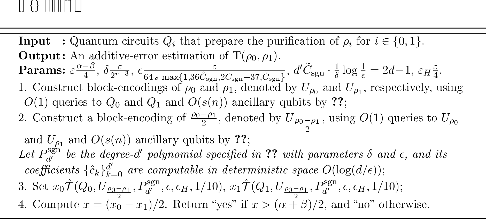
Let us demonstrate the correctness of 3 and analyze the computational complexity. We focus on the setting with \(s(n)=\Theta(\log{n})\). We set \(\varepsilon \mathrel{\vcenter{:}}= (\alpha-\beta)/4 \geq 2^{-O(s)}\) and assume that \(Q_0\) and \(Q_1\) are \(s(n)\)-qubit quantum circuits that prepare the purifications of \(\rho_0\) and \(\rho_1\), respectively. According to 18, we can construct \(O(s)\)-qubit quantum circuits \(U_{\rho_0}\) and \(U_{\rho_1}\) that encode \(\rho_0\) and \(\rho_1\) as \((1,O(s), 0)\)-block-encodings, using \(O(1)\) queries to \(Q_0\) and \(Q_1\) as well as \(O(1)\) one- and two-qubit quantum gates. Next, we apply 14 to construct a \((1,O(s),0)\)-block-encoding \(U_{\frac{\rho_0-\rho_1}{2}}\) of \(\frac{\rho_0 - \rho_1}{2}\), using \(O(1)\) queries to \(U_{\rho_0}\) and \(U_{\rho_1}\), as well as \(O(1)\) one- and two-qubit quantum gates.
Let \(\delta \mathrel{\vcenter{:}}= \frac{\varepsilon}{2^{r+3}}\), \(\epsilon \mathrel{\vcenter{:}}= \frac{\varepsilon}{64\,s\,\max\{1,36 \hat{C}_{\mathrm{sgn}},2 C_{\mathrm{sgn}}+37,\tilde{C}_{\mathrm{sgn}}\}}\),50 and \(d' \mathrel{\vcenter{:}}= \tilde{C}_{\mathrm{sgn}} \cdot \frac{1}{\delta} \log\frac{1}{\epsilon} \leq 2^{O(s(n))}\), where \(\tilde{C}_{\mathrm{sgn}}\) comes from 1. Let \(P_{d'}^{\mathrm{sgn}} \in \mathbb{R}[x]\) be the polynomial specified in 1 with \(d' = 2d-1\). Let \(\epsilon_H = \varepsilon/4\). By employing 3 (with \(\epsilon_1 \mathrel{\vcenter{:}}= 0\) and \(\epsilon_2 \mathrel{\vcenter{:}}= \epsilon\)) and the corresponding estimation procedure \(\hat{\mathcal{T}}(Q_i, U_{\frac{\rho_0-\rho_1}{2}}, P_{d'}^{\mathrm{sgn}}, \Theta(\epsilon), \epsilon_H, 1/10)\) from 17, we obtain the values \(x_i\) for \(i\in\{0,1\}\), ensuring the following inequalities: \[\label{eq:GapQSDlog-tester-pacc} \mathrm{Pr}\!\left[ \left| x_i - \mathrm{Tr}\left(P_{d'}^{\mathrm{sgn}}\Big(\frac{\rho_0-\rho_1}{2}\Big)\rho_i\right) \right| \leq (36 \hat{C}_{\mathrm{sgn}}\log{d'}+37)\epsilon + \epsilon_H \right] \geq 0.9 \text{ for } i\in\{0,1\}.\tag{38}\] Here, the implementation uses \(O(d^2 \log{d})\) queries to \(U_{\frac{\rho_0-\rho_1}{2}}\) and \(O(d^2 \log{d})\) multi-controlled single-qubit gates. Moreover, the circuit descriptions of \(\hat{\mathcal{T}}(Q_i, U_{\frac{\rho_0-\rho_1}{2}}, P_{d'}^{\mathrm{sgn}}, \epsilon, \epsilon_H, 1/10)\) can be computed in deterministic time \(\tilde{O}(d^{9/2}/\epsilon)\) and space \(O(s(n))\).
Now let \(x \mathrel{\vcenter{:}}= (x_0-x_1)/2\). We will finish the correctness analysis of 3 by showing \(\mathrm{Pr}\!\left[\left|x - \mathrm{T}(\rho_0, \rho_1)\right| \leq \varepsilon\right] > 0.8\) through 38 . By considering the approximation error of \(P_{d'}^{\mathrm{sgn}}\) in 1 and the QSVT implementation error in 3, we derive the following inequality in [prop:td-technical], whose proof is presented immediately afterward:
\(\mathrm{Pr}\!\left[\left|x - \mathrm{T}(\rho_0, \rho_1)\right| \leq (36 \hat{C}_{\mathrm{sgn}} \log{d'} +2 C_{\mathrm{sgn}}+37)\epsilon + \epsilon_H + 2^{r+1} \delta\right] > 0.8\).
Under the aforementioned choice of \(\delta\), \(\epsilon\), and \(\epsilon_H\), we have \(\epsilon_{H} = \varepsilon/4\), \(2^{r+1}\delta = \varepsilon/4\), and \((36 \hat{C}_{\mathrm{sgn}} \log{d'} +2 C_{\mathrm{sgn}}+37)\epsilon \leq \varepsilon/2\), and thus, \(\mathrm{Pr}\!\left[\left|x - \mathrm{T}(\rho_0, \rho_1)\right|\right] > 0.8\).
Finally, we analyze the computational resources required for 3. According to 17, we can compute \(x\) in BQL, with the resulting algorithm requiring \(O(d^2 \log{d} /\epsilon_H^2) = \tilde{O}(2^{2r}/\varepsilon^4)\) queries to \(Q_0\) and \(Q_1\). In addition, its circuit description can be computed in deterministic time \(\tilde{O}(d^{9/2}/\varepsilon) = \tilde{O}(2^{4.5r}/\varepsilon^{5.5})\). ◻
Proof of [prop:td-technical]. Using the triangle inequality, we obtain the following: \[\begin{align} \left| \frac{x_0-x_1}{2} - \mathrm{T}(\rho_0, \rho_1) \right| & = \left| \frac{x_0-x_1}{2} - \mathrm{Tr}\Big( \frac{\rho_0 - \rho_1}{2} \mathrm{sgn}\Big(\frac{\rho_0 - \rho_1}{2}\Big) \Big) \right| \\ & \leq \left| \frac{x_0-x_1}{2} - \mathrm{Tr}\Big(\frac{\rho_0-\rho_1}{2} P_{d'}^{\mathrm{sgn}}\Big(\frac{\rho_0-\rho_1}{2}\Big)\Big) \right| \\ & \qquad + \left| \mathrm{Tr}\Big(\frac{\rho_0-\rho_1}{2} P_{d'}^{\mathrm{sgn}}\Big(\frac{\rho_0-\rho_1}{2}\Big)\Big) - \mathrm{Tr}\Big( \frac{\rho_0 - \rho_1}{2} \mathrm{sgn}\Big(\frac{\rho_0 - \rho_1}{2}\Big) \Big) \right|. \end{align}\]
For the first term, by noting the QSVT implementation error in 3, we know by 38 that, with probability at least \(0.9^2 > 0.8\), it holds that \[\label{eq:td-first-term} \left| \frac{x_0-x_1}{2} - \mathrm{Tr}\Big(\frac{\rho_0-\rho_1}{2} P_{d'}^{\mathrm{sgn}}\Big(\frac{\rho_0-\rho_1}{2}\Big)\Big) \right| \leq (36 \hat{C}_{\mathrm{sgn}} \log{d'} +37)\epsilon + \epsilon_H.\tag{39}\] For the second term, let \(\frac{\rho_0-\rho_1}{2} = \sum_{j} \lambda_j \lvert{\psi_j}\rangle \langle{\psi_j}\rvert\), where \(\{ \lvert{\psi_j}\rangle \}\) is an orthonormal basis. Then, \[\label{eq:td-second-term} \left| \mathrm{Tr}\Big(\frac{\rho_0\!-\!\rho_1}{2} P_{d'}^{\mathrm{sgn}}\Big(\frac{\rho_0\!-\!\rho_1}{2}\Big)\Big) - \mathrm{Tr}\Big( \frac{\rho_0 \!-\! \rho_1}{2} \mathrm{sgn}\Big(\frac{\rho_0 \!-\! \rho_1}{2}\Big) \Big) \right| \leq \sum_j \left| \lambda_j P_{d'}^{\mathrm{sgn}}(\lambda_j) \!-\! \lambda_j \mathrm{sgn}(\lambda_j) \right|.\tag{40}\] We split the summation over \(j\) into three separate summations: \[\sum_j = \sum_{\lambda_j < -\delta} + \sum_{\lambda_j > \delta} + \sum_{-\delta \leq \lambda_j \leq \delta}.\] By noticing the approximation error of \(P_{d'}^{\mathrm{sgn}}\) in 1 and \(\sum_j |\lambda_j| = \mathrm{T}(\rho_0,\rho_1) \leq 1\), we obtain the following results for each of the three summations: \[\sum_{\lambda_j > \delta} \left| \lambda_j P_{d'}^{\mathrm{sgn}}(\lambda_j) - \lambda_j \mathrm{sgn}(\lambda_j) \right| = \sum_{\lambda_j > \delta} |\lambda_j| \left| P_{d'}^{\mathrm{sgn}}(\lambda_j) - 1 \right| \leq \sum_{\lambda_j > \delta} |\lambda_j| C_{\mathrm{sgn}} \epsilon \leq C_{\mathrm{sgn}} \epsilon,\] \[\sum_{\lambda_j < -\delta} \left| \lambda_j P_{d'}^{\mathrm{sgn}}(\lambda_j) - \lambda_j \mathrm{sgn}(\lambda_j) \right| = \sum_{\lambda_j < -\delta} |\lambda_j| \left| P_{d'}^{\mathrm{sgn}}(\lambda_j) + 1 \right| \leq \sum_{\lambda_j < -\delta} |\lambda_j| C_{\mathrm{sgn}} \epsilon \leq C_{\mathrm{sgn}} \epsilon,\] \[\sum_{-\delta \leq \lambda_j \leq \delta} \left| \lambda_j P_{d'}^{\mathrm{sgn}}(\lambda_j) - \lambda_j \mathrm{sgn}(\lambda_j) \right| \leq \sum_{-\delta \leq \lambda_j \leq \delta} 2|\lambda_j| \leq 2^{r+1}\delta.\] Hence, we derive the following inequality by summing over the aforementioned three inequalities: \[\label{eq:td-last-term} \sum_j \left| \lambda_j P_{d'}^{\mathrm{sgn}}(\lambda_j) - \lambda_j \mathrm{sgn}(\lambda_j) \right| \leq 2^{r+1} \delta + 2 C_{\mathrm{sgn}} \epsilon.\tag{41}\] By combining [eq:td-first-term,eq:td-second-term,eq:td-last-term], we conclude that \[\left|\frac{x_0-x_1}{2} - \mathrm{T}(\rho_0, \rho_1)\right| \leq (36 \hat{C}_{\mathrm{sgn}} \log{d'} + 37)\epsilon + \epsilon_H + 2 C_{\mathrm{sgn}} \epsilon + 2^{r+1} \delta. \qedhere\] ◻
4.3 GapQEDlog and GapQJSlog are in BQL↩︎
In this subsection, we will demonstrate 11 by devising a quantum algorithm that encompasses testers \(\mathcal{T}(Q_i, U_{\rho_i},P_{d'}^{\ln},\epsilon)\) for \(i \in \{0,1\}\), where the construction of testers employs the space-efficient QSVT associated with the normalized logarithmic function. Consequently, we can deduce that GapQJSlog is in BQL via a reduction from GapQJSlog to GapQEDlog.
Theorem 11. For any deterministic logspace computable function \(g(n)\) that satisfies \(g(n) \geq 1/\mathop{\mathrm{poly}}(n)\), we have that \(\texorpdfstring{\textrm{\mathrm{\small GapQED}\textsubscript{log}}}[g(n)]\) is in BQL.
Proof. We begin with a formal algorithm in 4.
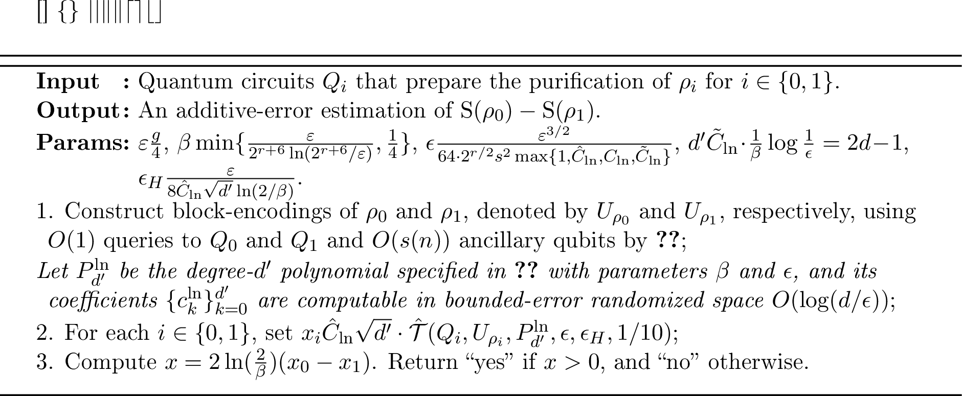
Let us now demonstrate the correctness and computational complexity of 4. We concentrate on the scenario with \(s(n) = \Theta(\log{n})\) and \(\varepsilon = g/4 \geq 2^{-O(s)}\). Our strategy is to estimate the entropy of each of \(\rho_0\) and \(\rho_1\), respectively. We assume that \(Q_0\) and \(Q_1\) are \(s\)-qubit quantum circuits that prepare the purifications of \(\rho_0\) and \(\rho_1\), respectively. By 18, we can construct \((1,O(s), 0)\)-block-encodings \(U_{\rho_0}\) and \(U_{\rho_1}\) of \(\rho_0\) and \(\rho_1\), respectively, using \(O(1)\) queries to \(Q_0\) and \(Q_1\) as well as \(O(1)\) one- and two-qubit quantum gates.
Let \(\beta = \min\{ \frac{\varepsilon}{2^{r+6} \ln(2^{r+6}/\varepsilon)}, \frac{1}{4} \}\), \(\epsilon \mathrel{\vcenter{:}}= \frac{\varepsilon^{3/2}}{64\cdot 2^{r/2}s^2\max\{1,\hat{C}_{\ln},C_{\ln},\tilde{C}_{\ln}\}}\), and \(d' \mathrel{\vcenter{:}}= \tilde{C}_{\ln} \cdot \frac{1}{\beta} \log \frac{1}{\epsilon} = 2^{O(s(n))}\), where \(\tilde{C}_{\ln}\) comes from 2. Let \(P_{d'}^{\ln} \in \mathbb{R}[x]\) be the polynomial specified in 2 with \(d' = 2d-1\). Let \(\epsilon_H \mathrel{\vcenter{:}}= \frac{\varepsilon}{8\hat{C}_{\ln}\sqrt{d'}\ln(2/\beta)}\). By utilizing 4 (with \(\epsilon_1 \mathrel{\vcenter{:}}= 0\) and \(\epsilon_2 \mathrel{\vcenter{:}}= \epsilon\)) and the corresponding estimation procedure \(\hat{\mathcal{T}}(Q_i, U_{\rho_i}, P_{d'}^{\ln}, \epsilon, \epsilon_H, 1/10)\) from 17, we obtain the values \(x_i\) for \(i\in\{0,1\}\), ensuring the following inequalities: \[\label{eq:GapQEDlog-tester-pacc} \mathrm{Pr}\!\left[ \left| x_i - \mathrm{Tr}\left(P_{d'}^{\ln}\!\left(\rho_i\right)\rho_i\right) \right| \leq \hat{C}_{\ln} \sqrt{d'} \rbra{\epsilon + \epsilon_H} \right] \geq 0.9 \text{ for } i\in\{0,1\}.\tag{42}\] Here, the implementation uses \(O(d^2)\) queries to \(U_{\rho_i}\) and \(O(d^2)\) multi-controlled single-qubit gates. Moreover, the circuit descriptions of \(\hat{\mathcal{T}}(Q_i, U_{\rho_i}, P_{d'}^{\ln}, \epsilon, \epsilon_H, 1/10)\) can be computed in bounded-error time \(\tilde{O}(d^{9}/\epsilon^4)\) and space \(O(s(n))\).
We will finish the correctness analysis of 4 by showing \(\mathrm{Pr}\!\left[\left| 2 \ln\rbra[\big]{\tfrac{2}{\beta}} x_i - \mathrm{S}(\rho_i)\right| \leq \varepsilon\right] \geq 0.9\) through 42 . By considering the approximation error of \(P_{d'}^{\ln}\) in 2 and the QSVT implementation error in 4, we derive the following inequality in [prop:entropy-technical], the proof of which is presented immediately afterward:
The following inequality holds for \(i \in \{0,1\}\): \[\mathrm{Pr}\Big[\left| 2 \ln\!\big(\tfrac{2}{\beta}\big) x_i - \mathrm{S}(\rho_i) \right| \leq 2 \ln\!\big(\tfrac{2}{\beta}\big) \rbra*{ \hat{C}_{\ln}\sqrt{d'}(\epsilon+\epsilon_H)+C_{\ln}\epsilon+2^{r+1}\beta} \Big] \geq 0.9.\]
Consequently, it is left to show that \(2 \ln\!\big(\tfrac{2}{\beta}\big) \rbra*{ \hat{C}_{\ln}\sqrt{d'}(\epsilon+\epsilon_H)+C_{\ln}\epsilon+2^{r+1}\beta} \leq \varepsilon\) for the specified value of \(\beta\), \(\epsilon\), and \(\epsilon_H\). This can be seen by noting that \[2\ln\rbra[\big]{\tfrac{2}{\beta}} \hat{C}_{\ln} \sqrt{d'} \epsilon_{H} = \tfrac{\varepsilon}{4}, \quad 2\ln\rbra[\big]{\tfrac{2}{\beta}} (\hat{C}_{\ln}\sqrt{d'} + C_{\ln}) \epsilon \leq \tfrac{\varepsilon}{2}, \quad\text{and}\quad 2 \ln\rbra[\big]{\tfrac{2}{\beta}} \cdot 2^{r+1} \beta \leq \tfrac{\varepsilon}{4}.\] The first identity and the second inequality are trivial. The third inequality, stated in [prop:GapQEDlog-beta-bound], is accompanied by a proof presented immediately afterward:
\(2 \ln(\frac{2}{\beta}) \cdot 2^{r+1} \beta \leq \tfrac{\varepsilon}{4}\).
Finally, we analyze the computational resources required for 4. As per 17, we can compute \(x\) in BQL, with the resulting algorithm requiring \(O(d^2/\epsilon_H^2) = \tilde{O}(2^{3r}/\varepsilon^5)\) queries to \(Q_0\) and \(Q_1\). Furthermore, its circuit description can be computed in bounded-error randomized time \(\tilde{O}(d^{9}/\epsilon^4) = \tilde{O}(2^{11r}/\varepsilon^{15})\). ◻
GapQJSlog is in BQL.
We can achieve \(\texorpdfstring{\textrm{\mathrm{\small GapQJS}\textsubscript{log}}}\in \textrm{\textsf{BQL}}\) by employing the estimation procedure \(\hat{\mathcal{T}}\) in 4 for three corresponding states, given that the quantum Jensen-Shannon divergence \(\mathrm{QJS}(\rho_0,\rho_1)\) is a linear combination of \(\mathrm{S}(\rho_0), \mathrm{S}(\rho_1)\), and \(\mathrm{S}\big(\frac{\rho_0+\rho_1}{2}\big)\). Nevertheless, the logspace Karp reduction from GapQJSlog to GapQEDlog (6) allows us to utilize \(\hat{\mathcal{T}}\) for only two states.51 Furthermore, our construction is adapted from the time-bounded scenario [40].
Corollary 6. For any functions \(\alpha(n)\) and \(\beta(n)\) that can be computed in deterministic logspace and satisfy \(\alpha(n)-\beta(n) \geq 1/\mathop{\mathrm{poly}}(n)\), we have that \(\texorpdfstring{\textrm{\mathrm{\small GapQJS}\textsubscript{log}}}[\alpha(n),\beta(n)]\) is in BQL.
Proof. Let \(Q_0\) and \(Q_1\) be the given \(s(n)\)-qubit quantum circuits where \(s(n)=\Theta(\log{n})\). Consider a classical-quantum mixed state on a classical register \(\mathsf{B}\) and a quantum register \(\mathsf{Y}\), denoted by \(\rho'_1 \mathrel{\vcenter{:}}= \frac{1}{2}\lvert{0}\rangle\langle{0}\rvert\otimes \rho_0 + \frac{1}{2} \lvert{1}\rangle\langle{1}\rvert\otimes \rho_1\), where \(\rho_0\) and \(\rho_1\) are states obtained by running \(Q_0\) and \(Q_1\), respectively, and tracing out the non-output qubits. We utilize our reduction to output classical-quantum mixed states \(\rho'_0\) and \(\rho'_1\), which are the output of \((s+2)\)-qubit quantum circuits \(Q'_0\) and \(Q'_1\),52 respectively, where \(\rho'_0\mathrel{\vcenter{:}}=(p_0\lvert{0}\rangle\langle{0}\rvert+p_1\lvert{1}\rangle\langle{1}\rvert)\otimes(\frac{1}{2}\rho_0+\frac{1}{2}\rho_1)\) and \(\mathsf{B}'\mathrel{\vcenter{:}}=(p_0,p_1)\) is an independent random bit with entropy \(\mathrm{H}(\mathsf{B}')=1-\frac{1}{2}[\alpha(n)+\beta(n)]\). Let \(\mathrm{S}_2(\rho)\mathrel{\vcenter{:}}=\mathrm{S}(\rho)/\ln{2}\) for any quantum state \(\rho\), we then have derived that: \[\label{eq:QJS-to-QED} \begin{align} \mathrm{S}_2(\rho'_0)-\mathrm{S}_2(\rho'_1) &= \mathrm{S}_2(\mathsf{B}',\mathsf{Y})_{\rho'_0} - \mathrm{S}_2(\mathsf{B},\mathsf{Y})_{\rho'_1}\\ &= [\mathrm{H}(\mathsf{B}')+\mathrm{S}_2(\mathsf{Y}|\mathsf{B}')_{\rho'_0}]-[\mathrm{H}(\mathsf{B})+\mathrm{S}_2(\mathsf{Y}|\mathsf{B})_{\rho'_1}]\\ &= \mathrm{S}_2(\mathsf{Y})_{\rho'_0} - \mathrm{S}_2(\mathsf{Y}|\mathsf{B})_{\rho'_1} + \mathrm{H}(\mathsf{B}') - \mathrm{H}(\mathsf{B})\\ &= \mathrm{S}_2(\mathsf{Y})_{\rho'_0}-\mathrm{S}_2(\mathsf{Y}|\mathsf{B})_{\rho'_1} -\tfrac{1}{2}[\alpha(n)+\beta(n)]\\ &= \mathrm{S}_2 \rbra*{ \tfrac{1}{2}\rho_0+\tfrac{1}{2}\rho_1 } - \tfrac{1}{2}(\mathrm{S}_2(\rho_0)+\mathrm{S}_2(\rho_1)) -\tfrac{1}{2}[\alpha(n)+\beta(n)]\\ &= \mathrm{QJS}_2(\rho_0,\rho_1) - \tfrac{1}{2}[\alpha(n)+\beta(n)]. \end{align}\tag{43}\] Here, the second line derives from the definition of quantum conditional entropy and acknowledges that both \(\mathsf{B}\) and \(\mathsf{B}'\) are classical registers. The third line owes to the independence of \(\mathsf{B}'\) as a random bit. Furthermore, the fifth line relies on the Joint entropy theorem (2).
By plugging 43 into the conditions in the promise of \(\textrm{\mathrm{\small GapQJS}}_{\log}[\alpha(n),\beta(n)]\), we can define \(g(n')\mathrel{\vcenter{:}}=\frac{\ln{2}}{2} \big( \alpha(n)-\beta(n) \big)\) and conclude that:
If \(\mathrm{QJS}_2(\rho_0,\rho_1) \geq \alpha(n)\), then \(\mathrm{S}(\rho'_0)-\mathrm{S}(\rho'_1) \geq \frac{\ln{2}}{2} \big( \alpha(n)-\beta(n) \big) = g(n')\);
If \(\mathrm{QJS}_2(\rho_0,\rho_1) \leq \beta(n)\), then \(\mathrm{S}(\rho'_0)-\mathrm{S}(\rho'_1) \leq -\frac{\ln{2}}{2} \big(\alpha(n)-\beta(n) \big) = -g(n')\).
As \(\rho'_1\) and \(\rho'_0\) are \(r'(n')\)-qubit states where \(n'\mathrel{\vcenter{:}}=3n\)53 and \(r'(n')\mathrel{\vcenter{:}}= r(n)+1\), the output length of the corresponding space-bounded quantum circuits \(Q'_0\) and \(Q'_1\) is \(r'(n')\). Hence, \(\textrm{\mathrm{\small GapQJS}}_{s}[\alpha,\beta]\) is logspace Karp reducible to \(\textrm{\mathrm{\small GapQED}}_{s+3}[g]\) by mapping \((Q_0,Q_1)\) to \((Q'_0,Q'_1)\). ◻
We next present the proofs of [prop:entropy-technical,prop:GapQEDlog-beta-bound]:
Proof of [prop:entropy-technical]. We only prove the case with \(i=0\) while the case with \(i=1\) follows straightforwardly. By applying the triangle inequality with \(i=0\), we have: \[\left| 2\ln\!\big(\tfrac{2}{\beta}\big) x_0 - \mathrm{S}(\rho_0) \right| \leq \left| 2\ln\!\big(\tfrac{2}{\beta}\big) x_0 - 2\ln\!\big(\tfrac{2}{\beta}\big) \mathrm{Tr}\left(P_{d'}^{\ln}(\rho_0)\rho_0\right) \right| + \left| 2\ln\!\big(\tfrac{2}{\beta}\big) \mathrm{Tr}\left(P_{d'}^{\ln}(\rho_0)\rho_0\right) - \mathrm{S}(\rho_0) \right|.\] For the first term, by noting the QSVT implementation error in 4, we have by 42 that with probability at least \(0.9\), it holds that \[\label{eq:entropy-first-term} \left| 2\ln\!\big(\tfrac{2}{\beta}\big) x_0 - 2 \ln\!\big(\tfrac{2}{\beta}\big) \mathrm{Tr}\rbra[\big]{P_{d'}^{\ln}(\rho_0)\rho_0} \right| \leq 2 \ln\!\big(\tfrac{2}{\beta}\big) \hat{C}_{\ln} \sqrt{d'} (\epsilon + \epsilon_H).\tag{44}\] For the second term, let \(\rho_0 = \sum_{j} \lambda_j \lvert{\psi_j}\rangle \langle{\psi_j}\rvert\), where \(\{ \lvert{\psi_j}\rangle \}\) is an orthonormal basis. Then, \[\label{eq:entropy-second-term} \left| 2\ln\!\big(\tfrac{2}{\beta}\big) \mathrm{Tr}\rbra[\big]{P_{d'}^{\ln}(\rho_0)\rho_0} - \mathrm{S}(\rho_0) \right| \leq \sum_j \left| 2 \ln\!\big(\tfrac{2}{\beta}\big) \lambda_j P_{d'}^{\ln}(\lambda_j) - \lambda_j \ln(1/\lambda_j) \right|.\tag{45}\] We split the summation over \(j\) into two separate summations: \(\sum_j = \sum_{\lambda_j > \beta} + \sum_{\lambda_j \leq \beta}.\) By noticing the approximation error of \(P_{d'}^{\ln}\) in 2 and \(\sum_{j} |\lambda_j| = \mathrm{Tr}(\rho_0) \leq 1\), we can then obtain the following results for each of the two summations: \[\begin{align} \sum_{\lambda_j > \beta} \left| 2\ln\!\big(\tfrac{2}{\beta}\big) \lambda_j P_{d'}^{\ln}(\lambda_j) - \lambda_j \ln(1/\lambda_j) \right| & = \sum_{\lambda_j > \beta} |\lambda_j| \cdot \left| 2 \ln\!\big(\tfrac{2}{\beta}\big) P_{d'}^{\ln}(\lambda_j) - \ln(1/\lambda_j) \right| \\ & \leq \sum_{\lambda_j > \beta} |\lambda_j| \cdot 2 \ln\!\big(\tfrac{2}{\beta}\big) C_{\ln} \epsilon \\ & \leq 2 \ln\!\big(\tfrac{2}{\beta}\big) C_{\ln} \epsilon, \end{align}\] \[\begin{align} \sum_{\lambda_j \leq \beta} \left| 2 \ln\!\big(\tfrac{2}{\beta}\big) \lambda_j P_{d'}^{\ln}(\lambda_j) - \lambda_j \ln(1/\lambda_j) \right| & \leq \sum_{\lambda_j \leq \beta} \left( 2 \ln\!\big(\tfrac{2}{\beta}\big) |\lambda_j| + |\lambda_j| \ln(1/\lambda_j) \right) \\ & \leq 2 \ln\!\big(\tfrac{2}{\beta}\big) \cdot 2^r \beta + 2^r \beta\ln(1/\beta)\\ & \leq 2\ln\!\big(\tfrac{2}{\beta}\big) 2^{r+1} \beta. \end{align}\] Hence, we have derived the following inequality by summing over the aforementioned inequalities: \[\label{eq:entropy-last-term} \sum_j \left| 2 \ln\!\big(\tfrac{2}{\beta}\big) \lambda_j P_{d'}^{\ln}(\lambda_j) - \lambda_j \ln(1/\lambda_j) \right| \leq 2 \ln\!\big(\tfrac{2}{\beta}\big) C_{\ln} \epsilon + 2\ln\!\big(\tfrac{2}{\beta}\big) 2^{r+1} \beta.\tag{46}\] By combining [eq:entropy-first-term,eq:entropy-second-term,eq:entropy-last-term], we conclude that \[\left| 2\ln\!\big(\tfrac{2}{\beta}\big) x_0 - \mathrm{S}(\rho_0) \right| \leq 2 \ln\!\big(\tfrac{2}{\beta}\big) \left( \hat{C}_{\ln}\sqrt{d'} \rbra[\big]{\epsilon + \epsilon_H} + C_{\ln} \epsilon + 2^{r+1} \beta \right). \qedhere\] ◻
Proof of [prop:GapQEDlog-beta-bound]. Note that the choice of \(\beta\) is given by \(\beta \mathrel{\vcenter{:}}= \frac{\varepsilon}{2^{r+6} \ln(\frac{2^{r+6}}{\varepsilon})}\). Then, to demonstrate the inequality \(2 \ln(\frac{2}{\beta}) \cdot 2^{r+1} \beta \leq \tfrac{\varepsilon}{4}\), it suffices to prove that \[\label{eq:GapQEDlog-beta-bound} 2 \ln\left(\frac{2^{r+7} \ln(\frac{2^{r+6}}{\varepsilon})}{\varepsilon}\right) \cdot \frac{\varepsilon}{2^{5} \ln(\frac{2^{r+6}}{\varepsilon})} \leq \frac{\varepsilon}{4}.\tag{47}\]
Let \(x \mathrel{\vcenter{:}}= 2^{-r-6} \varepsilon \in (0, 1)\), then 47 becomes \(\ln\left(\frac{2}{x} \ln\left(\frac{1}{x}\right)\right) \leq 4 \ln\left(\frac{1}{x}\right)\). This simplifies further to \(2x^3\ln\left(\frac{1}{x}\right) \leq 1\).
To complete the proof, let \(f(x) = 2x^3\ln(\frac{1}{x})\), then its first derivative is \(f'(x) = 2x^2 \left(3\ln\left(\frac{1}{x}\right)-1\right)\). Note that \(f'(x) > 0\) for \(x \in (0, e^{-1/3})\) and \(f'(x) < 0\) for \(x \in (e^{-1/3}, 1)\). Thus, \(f(x)\) is monotonically increasing for \(x \in (0, e^{-1/3})\) and monotonically decreasing for \(x \in (e^{-1/3}, 1)\). Therefore, \(f(x)\) takes the maximum value at \(x = e^{-1/3}\), and consequently, \(f(x) \leq f(e^{-1/3}) = \frac{2}{3e} \leq 1\). ◻
4.4 \(\overline{\mathrm{\small CertQSD}}\)log and \(\overline{\mathrm{\small CertQHS}}\)log are in coRQUL↩︎
To make the error one-sided, we adapt the Grover search when the number of solutions is one quarter [63], also known as the exact amplitude amplification [64].
Lemma 20 (Exact amplitude amplification, adapted from [64]). Suppose \(U\) is a unitary of interest such that \(U\lvert{\bar 0}\rangle = \sin(\theta) \lvert{\psi_0}\rangle + \cos(\theta) \lvert{\psi_1}\rangle\), where \(\lvert{\psi_0}\rangle\) and \(\lvert{\psi_1}\rangle\) are normalized pure states and \(\langle \psi_0 | \psi_1 \rangle = 0\). Let \(G = - U (I - 2\lvert{\bar 0}\rangle\langle{\bar 0}\rvert) U^\dagger (I - 2\lvert{\psi_0}\rangle\langle{\psi_0}\rvert)\) be the Grover operator. Then, for every integer \(j \geq 0\), we have \[G^j U \lvert{\bar 0}\rangle = \sin((2j+1)\theta) \lvert{\psi_0}\rangle + \cos((2j+1)\theta) \lvert{\psi_1}\rangle.\]
In particular, with a single application of \(G\), we obtain \[G U \lvert{\bar 0}\rangle = \sin(3\theta) \lvert{\psi_0}\rangle + \cos(3\theta) \lvert{\psi_1}\rangle,\] signifying that \(G U \lvert{\bar 0}\rangle = \lvert{\psi_0}\rangle\) when \(\sin(\theta) = 1/2\).
Notably, when dealing with the unitary of interest with the property specified in 20, which is typically a quantum algorithm with acceptance probability linearly dependent on the chosen distance-like measure (e.g., a tester \(\mathcal{T}\) from 17), 20 guarantees that the resulting algorithm \(\mathcal{A}\) accepts with probability exactly \(1\) for yes instances (\(\rho_0=\rho_1\)). However, achieving \(\mathcal{A}\) to accept with probability polynomially deviating from \(1\) for no instances requires additional efforts, leading to the coRQUL containment established through error reduction for coRQUL (5). In a nutshell, demonstrating coRQUL containment entails satisfying the desired property, which is achieved differently for \(\overline{\mathrm{\small CertQSD}}\)log and \(\overline{\mathrm{\small CertQHS}}\)log.
4.4.1 \(\overline{\mathrm{\small CertQSD}}\)log is in coRQUL↩︎
Our algorithm in 12 relies on the quantum tester \(\mathcal{T}(Q_i, U_{\frac{\rho_0-\rho_1}{2}},P_{d'}^{\mathrm{sgn}},\epsilon)\), which is specified in 3. According to [remark:QSVT-parity-preserving], the exact implementation of the space-efficient QSVT associated with odd polynomials preserves the original point. As a consequence, \(\mathcal{T}(Q_i, U_{\frac{\rho_0-\rho_1}{2}}, P_{d'}^{\mathrm{sgn}},\epsilon)\) outputs \(0\) with probability exactly \(1/2\) when \(\rho_0=\rho_1\), enabling us to derive the coRQUL containment through a relatively involved analysis for cases when \(\mathrm{T}(\rho_0,\rho_1) \geq \alpha\):
Theorem 12. For any deterministic logspace computable function \(\alpha(n) \geq 1/\mathop{\mathrm{poly}}(n)\), we have that \(\texorpdfstring{\textrm{\overline{\mathrm{\small CertQSD}}\textsubscript{log}}}[\alpha(n)]\) is in coRQUL.
Proof. We first present a formal algorithm in 5:
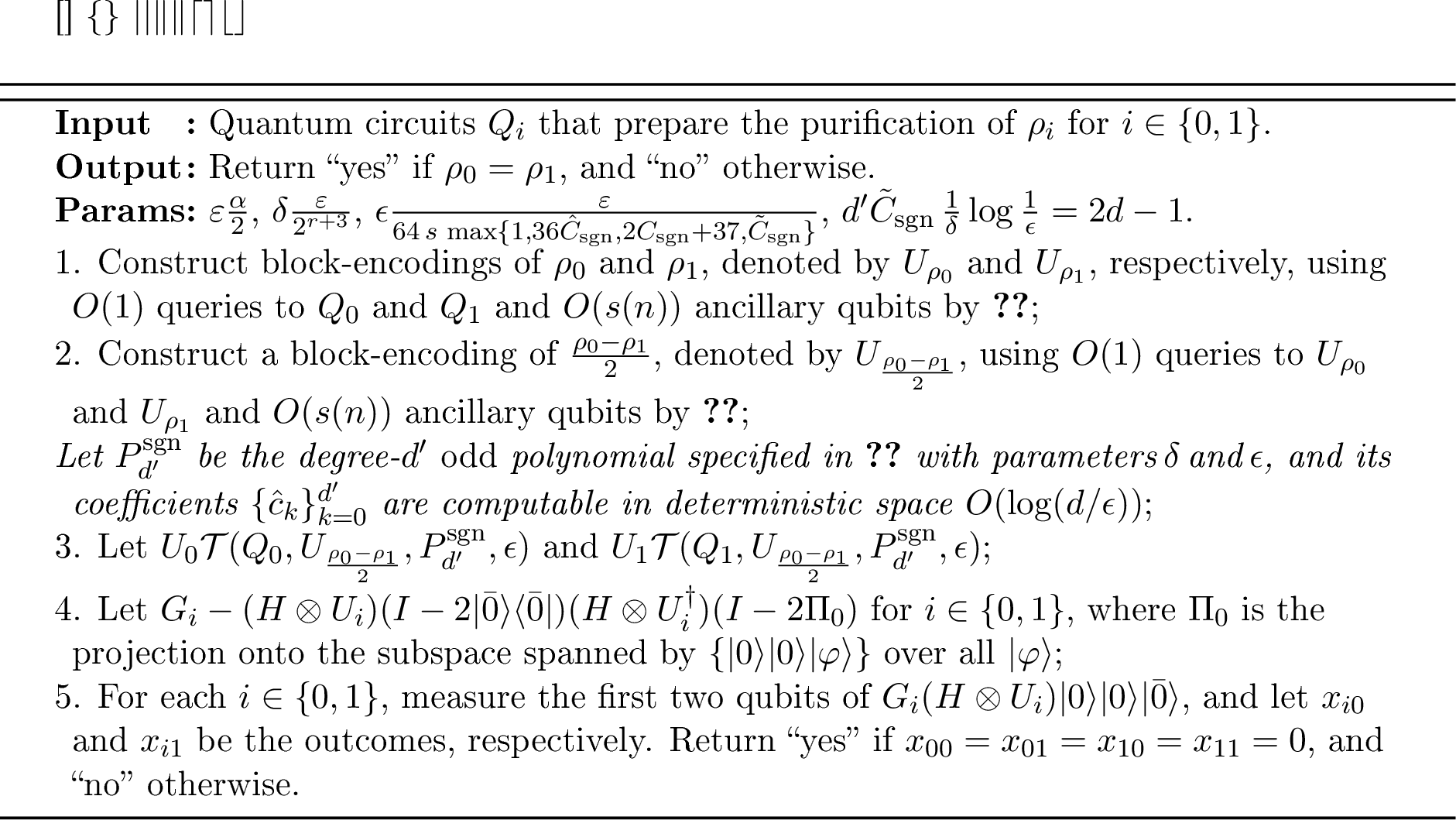
Constructing the unitary of interest via the space-efficient QSVT.
We consider the setting with \(s(n) = \Theta(\log{n})\) and \(\varepsilon = \alpha / 2\). Suppose \(Q_0\) and \(Q_1\) are \(s(n)\)-qubit quantum circuits that prepare the purifications of \(\rho_0\) and \(\rho_1\), respectively. Similar to 3, we first construct an \(O(s)\)-qubit quantum circuit \(U_{\frac{\rho_0 - \rho_1}{2}}\) that is a \((1,O(s), 0)\)-block-encoding of \(\frac{\rho_0-\rho_1}{2}\), using \(O(1)\) queries to \(Q_0\) and \(Q_1\) and \(O(1)\) one- and two-qubit quantum gates.
Let \(\delta = \frac{\varepsilon}{2^{r+3}}\), \(\epsilon \mathrel{\vcenter{:}}= \frac{\varepsilon}{64\,s\,\max\{1,36 \hat{C}_{\mathrm{sgn}},2 C_{\mathrm{sgn}}+37,\tilde{C}_{\mathrm{sgn}}\}}\), and \(d' \mathrel{\vcenter{:}}= \tilde{C}_{\mathrm{sgn}} \cdot \frac{1}{\delta} \log\frac{1}{\epsilon} = 2^{O(s(n))}\), where \(\tilde{C}_{\mathrm{sgn}}\) comes from 1. Let \(P_{d'}^{\mathrm{sgn}} \in \mathbb{R}[x]\) be the odd polynomial specified in 1. Let \(U_i \mathrel{\vcenter{:}}= \mathcal{T}(Q_i, U_{\frac{\rho_0-\rho_1}{2}}, P_{d'}^{\mathrm{sgn}}, \epsilon)\) for \(i \in \{0,1\}\), then we have the following equalities: \[\forall i\in\{0,1\}, \quad U_i \lvert{0}\rangle\lvert{\bar 0}\rangle = \sqrt{p_i} \lvert{0}\rangle \lvert{\psi_{i,0}}\rangle + \sqrt{1 - p_i} \lvert{1}\rangle \lvert{\psi_{i,1}}\rangle, \quad\text{where } 0 \leq p_i \leq 1.\]
Let \(H\) be the Hadamard gate, then we derive the following equality for \(i\in\{0,1\}\): \[(H \otimes U_i) \lvert{0}\rangle \lvert{0}\rangle\lvert{\bar 0}\rangle = \sqrt{\frac{p_i}{2}} \lvert{0}\rangle\lvert{0}\rangle\lvert{\psi_{i,0}}\rangle + \underbrace{\sqrt{\frac{p_i}{2}} \lvert{1}\rangle\lvert{0}\rangle\lvert{\psi_{i,0}}\rangle + \sqrt{\frac{1-p_i}{2}} \lvert{0}\rangle\lvert{1}\rangle\lvert{\psi_{i,1}}\rangle + \sqrt{\frac{1-p_i}{2}} \lvert{1}\rangle\lvert{1}\rangle\lvert{\psi_{i,1}}\rangle}_{\sqrt{1 - \frac{p_i}{2}}\lvert{\perp_i}\rangle}.\]
Making the error one-sided by exact amplitude amplification.
Consider the Grover operator \(G_i \mathrel{\vcenter{:}}= - (H \otimes U_i) (I - 2\lvert{\bar 0}\rangle\langle{\bar 0}\rvert) (H \otimes U_i^\dagger) (I - 2\Pi_0)\), where \(\Pi_0\) is the projection onto the subspace spanned by \(\{ \lvert{0}\rangle\lvert{0}\rangle\lvert{\varphi}\rangle \}\) over all \(\lvert{\varphi}\rangle\). By employing the exact amplitude amplification (20), we can obtain that: \[\label{eq:exact-AA-coCertQSDlog} \begin{align} G_i (H \otimes U_i) \lvert{0}\rangle\lvert{0}\rangle\lvert{\bar 0}\rangle &= \sin(3\theta_i) \lvert{0}\rangle\lvert{0}\rangle\lvert{\psi_{i,0}}\rangle + \cos(3\theta_i) \lvert{\perp_i}\rangle,\\ \text{where } \sin^2(\theta_i) &= \frac{p_i}{2} \text{ when } \theta_i \in \sbra*{0, \frac{\pi}{4}}. \end{align}\tag{48}\] Let \(x_{i0}\) and \(x_{i1}\) be the measurement outcomes of the first two qubits of \(G_i (H \otimes U_i) \lvert{0}\rangle\lvert{0}\rangle\lvert{\bar 0}\rangle\) for \(i\in\{0,1\}\). 5 returns “yes” if \(x_{00} = x_{01} = x_{10} = x_{11} = 0\), and “no” otherwise. Let \(U_{P_{d'}^{\mathrm{sgn}}\left(\frac{\rho_0 - \rho_1}{2}\right)}\) be the unitary operator being controlled in the implementation of \(U_i \mathrel{\vcenter{:}}= \mathcal{T}(Q_i, U_{\frac{\rho_0-\rho_1}{2}}, P_{d'}^{\mathrm{sgn}}, \epsilon)\), and note that by 3, \(U_{P_{d'}^{\mathrm{sgn}}\left(\frac{\rho_0 - \rho_1}{2}\right)}\) is a \((1, O(s), (36 \hat{C}_{\mathrm{sgn}} \log{d'} + 37)\epsilon)\)-block-encoding of \(P_{d'}^{\mathrm{sgn}}\left(\frac{\rho_0-\rho_1}{2}\right)\). We will show the correctness of our algorithm as follows:
For yes instances (\(\rho_0=\rho_1\)), \(U_{P_{d'}^{\mathrm{sgn}}\left(\frac{\rho_0 - \rho_1}{2}\right)}\) is a \((1,O(s), 0)\)-block-encoding of the zero operator, following from [remark:QSVT-parity-preserving]. Consequently, \(\mathcal{T}(Q_i, U_{\frac{\rho_0-\rho_1}{2}}, P_{d'}^{\mathrm{sgn}}, \epsilon)\) outputs \(0\) with probability \(1/2\) for \(i \in \{0,1\}\), i.e., \(p_0=p_1=1/2\). As a result, we have \(\theta_0 = \theta_1 = \pi/6\) and \(\sin^2(3\theta_0) = \sin^2(3\theta_1) = 1\). Substituting these values into 48 , we can conclude that \(x_{00} = x_{01} = x_{10} = x_{11} = 0\) with certainty, which completes the analysis.
For no instances (\(\mathrm{T}(\rho_0, \rho_1) \geq \alpha\)), \(U_{P_{d'}^{\mathrm{sgn}}\left(\frac{\rho_0 - \rho_1}{2}\right)}\) is a \((1,O(s), 0)\)-block-encoding of \(A\) satisfying \[\left\| A - P_{d'}^{\mathrm{sgn}}\left(\frac{\rho_0-\rho_1}{2}\right) \right\| \leq (36 \hat{C}_{\mathrm{sgn}} \log{d'} +37)\epsilon.\] Let \(p_i\) be the probability that \(\mathcal{T}(Q_i, U_{\frac{\rho_0-\rho_1}{2}}, P_{d'}^{\mathrm{sgn}}, \epsilon)\) outputs \(0\) for \(i \in \{0,1\}\), then \(p_i = \frac{1}{2}\big(1+\operatorname{Re}(\mathrm{Tr}(\rho_i A))\big)\) following from 17. A direct calculation similar to [prop:td-technical] indicates that: \[\left| (p_0 - p_1) - \mathrm{T}(\rho_0, \rho_1) \right| \leq (36 \hat{C}_{\mathrm{sgn}}\log{d'}+2 C_{\mathrm{sgn}}+37)\epsilon + 2^{r+1} \delta.\] Under the choice of \(\delta\) and \(\epsilon\) (the same as in the proof of 10), we obtain that \(|(p_0 - p_1) - \mathrm{T}(\rho_0, \rho_1)| \leq \varepsilon\) which yields that \(\max\{ |p_0-1/2|, |p_1-1/2| \} \geq \varepsilon/2\).54
Noting that \(\mathrm{Pr}\!\left[x_{i0}=x_{i1}=0\right]=\sin^2(3\theta_i)\) for \(i \in \{0,1\}\), 5 will return “yes” with probability \(p_{{\rm yes}} = \sin^2(3\theta_0) \sin^2(3\theta_1)\). We provide an upper bound for \(p_{{\rm yes}}\) in [prop:coCertQSDlog-soundness-upper-bound], with the proof provided immediately afterward:
Let \(f(\theta_0,\theta_1) \mathrel{\vcenter{:}}= \sin^2(3\theta_0) \sin^2(3\theta_1)\) be a function such that \(\sin^2(\theta_i) = p_i/2\) for \(i\in\{0,1\}\) and \(\max\{ |p_0-1/2|, |p_1-1/2| \} \geq \varepsilon/2\), then \(f(\theta_0,\theta_1) \leq 1 - \varepsilon^2/4\).
Consequently, we finish the analysis by noticing \(p_{{\rm yes}} = f(\theta_0,\theta_1) \leq 1 - \varepsilon^2/4 = 1 - \alpha^2/16\).
Now we analyze the complexity of 5. Following 17, we can compute \(x_{00}, x_{01}, x_{10}, x_{11}\) in BQL. The quantum circuit that computes \(x_{00}, x_{01}, x_{10}, x_{11}\) takes \(O(d^2 \log{d}) = \tilde{O}(2^{2r}/\alpha^2)\) queries to \(Q_0\) and \(Q_1\), and its circuit description can be computed in deterministic time \(\tilde{O}(d^{9/2}/\alpha) = \tilde{O}(2^{4.5r}/\alpha^{5.5})\). Finally, we conclude the coRQUL containment of \(\overline{\mathrm{\small CertQSD}}\)log by applying error reduction for coRQUL (5) to 5. ◻
Proof of [prop:coCertQSDlog-soundness-upper-bound]. We begin by stating the facts that \(\sin^2(\theta_i) = p_i/2\) for \(i \in \{0,1\}\) and \(\sin^2(3\theta) = \sin^6(\theta) - 6\cos^2(\theta) \sin^4(\theta) + 9\cos^4(\theta)\sin^2(\theta)\). Then we notice that \(0 \leq p_0,p_1 \leq 1\) and complete the proof by a direct calculation: \[\begin{align} f(\theta_0,\theta_1) & = \left( 2p_0^3 - 6p_0^2 + \tfrac{9}{2} p_0 \right) \left( 2p_1^3 - 6p_1^2 + \tfrac{9}{2} p_1 \right) \\ & \leq \left( 1 - \left( p_0 - \tfrac{1}{2} \right)^2 \right) \left( 1 - \left( p_1 - \tfrac{1}{2} \right)^2 \right) \\ & \leq 1 - \left( \max\left\{\left|p_0 - \tfrac{1}{2}\right|, \left|p_1 - \tfrac{1}{2}\right|\right\} \right)^2 \\ & \leq 1 - \tfrac{\varepsilon^2}{4}. \qedhere \end{align}\] ◻
4.4.2 \(\overline{\mathrm{\small CertQHS}}\)log is in coRQUL↩︎
As a warm-up, we observe that \(\mathrm{HS}^2(\rho_0,\rho_1)\) can be written as a summation of \(\frac{1}{2}\mathrm{Tr}(\rho_0^2)\), \(\frac{1}{2}\mathrm{Tr}(\rho_1^2)\), and \(-\mathrm{Tr}(\rho_0\rho_1)\). It follows that GapQHSlog is contained in BQL:
Theorem 13. For any functions \(\alpha(n)\) and \(\beta(n)\) that can be computed in deterministic logspace and satisfy \(\alpha(n)-\beta(n) \geq 1/\mathop{\mathrm{poly}}(n)\), we have that \(\textrm{\mathrm{\small GapQHS}}_{\log}[\alpha(n),\beta(n)]\) is in BQL.
Proof. Note that \(\mathrm{HS}^2(\rho_0,\rho_1) = \frac{1}{2} \left(\mathrm{Tr}(\rho_0^2)+\mathrm{Tr}(\rho_1^2)\right)-\mathrm{Tr}(\rho_0\rho_1)\). Let \(\varepsilon \mathrel{\vcenter{:}}= (\alpha - \beta)/100\). According to 9, we can use the SWAP test to estimate \(\mathrm{Tr}(\rho_0^2)\), \(\mathrm{Tr}(\rho_1^2)\), and \(\mathrm{Tr}(\rho_0\rho_1)\), and hence \(\mathrm{HS}^2(\rho_0,\rho_1)\), within additive error \(\varepsilon\) with high probability by performing \(O(1/\varepsilon^2)\) sequential repetitions. Therefore, we can conclude that \(\textrm{\mathrm{\small GapQHS}}_{\log}[\alpha(n),\beta(n)]\) is in BQL. ◻
The observing algorithm in 13 corresponds to a single quantum circuit that uses two random coins, implementable by single-qubit measurements in the computational basis, and whose acceptance probability is proportional to \(\mathrm{HS}^2(\rho_0,\rho_1)\). However, to guarantee unitarity, we construct an alternative algorithm using the LCU technique, which serves as the unitary of interest with the desired property.
Theorem 14. For any deterministic logspace computable function \(\alpha(n) \geq 1/\mathop{\mathrm{poly}}(n)\), we have that \(\texorpdfstring{\textrm{\overline{\mathrm{\small CertQHS}}\textsubscript{log}}}[\alpha(n)]\) is in coRQUL.
Proof. We first provide a formal algorithm in 6.

Constructing the unitary of interest via the SWAP test.
We consider the setting with \(s(n)=\Theta(\log(n))\). Our main building block is the circuit implementation of the SWAP test (9). Specifically, we utilize the subroutine \(\textrm{\mathrm{\small SWAP}}(\rho_i,\rho_j)\) for \(i,j\in \{0,1\}\), which involves applying \(Q_i\) and \(Q_j\) to prepare quantum states \(\rho_i\) and \(\rho_j\), respectively, and then employing the SWAP test on these states \(\rho_i\) and \(\rho_j\). We denote by \(p_{ij}\) the probability that \(\textrm{\mathrm{\small SWAP}}(\rho_i,\rho_j)\) outputs \(0\) based on the measurement outcome of the control qubit in the SWAP test. Following 9, we have \(p_{ij} = \frac{1}{2}\big(1+\mathrm{Tr}(\rho_i\rho_j) \big)\) for \(i,j \in \{0,1\}\).
We define \(T_{ij}\mathrel{\vcenter{:}}=\textrm{\mathrm{\small SWAP}}(\rho_i,\rho_j)\) for \((i,j) \in \mathcal{I}\mathrel{\vcenter{:}}=\{(0,0), (1,1), (0,1)\}\), with the control qubit in \(\textrm{\mathrm{\small SWAP}}(\rho_i,\rho_j)\) serving as the output qubit of \(T_{ij}\). By introducing another ancillary qubit, we construct \(T'_{ij} \mathrel{\vcenter{:}}= \textrm{\mathrm{\small CNOT}}(I \otimes T_{ij})\) for \((i,j) \in \mathcal{I}\), where \(\textrm{\mathrm{\small CNOT}}\) is controlled by the output qubit of \(T_{ij}\) and targets on the new ancillary qubit. It is effortless to see that \(T'_{ij}\) prepares the purification of \(\varrho(p_{ij})\) with \(\varrho(p_{ij})\mathrel{\vcenter{:}}= p_{ij} \lvert{0}\rangle\langle{0}\rvert + (1-p_{ij})\lvert{1}\rangle\langle{1}\rvert\) for \((i,j)\in\mathcal{I}\).
By applying 18, we can construct quantum circuits \(T''_{ij}\) for \((i,j)\in\mathcal{I}\) that serve as \((1, O(s), 0)\)-block-encoding of \(\varrho(p_{ij})\), using \(O(1)\) queries to \(T'_{ij}\) and \(O(1)\) one- and two-qubit quantum gates. Notably, \((X \otimes I) T''_{01}\), with \(X\) acting on the qubit of \(\varrho(p_{01})\), prepares the purification of \(X \varrho(p_{01}) X^\dagger = p_{01}\lvert{1}\rangle\langle{1}\rvert + (1-p_{01})\lvert{0}\rangle\langle{0}\rvert = \varrho(1-p_{01})\), leading to the equality: \[\varrho(\rho_0,\rho_1)\mathrel{\vcenter{:}}= \frac{1}{4} \varrho(p_{00}) + \frac{1}{4} \varrho(p_{11}) + \frac{1}{2} \varrho(1-p_{01}) = \varrho\!\left(\frac{1}{2} + \frac{\mathrm{HS}^2(\rho_0, \rho_1)}{4}\right).\]
Consequently, we employ 14 to construct a unitary quantum circuit \(U\) that is a \((1,m, 0)\)-block-encoding of \(\varrho\big(\frac{1}{2} + \frac{\mathrm{HS}^2(\rho_0, \rho_1)}{4}\big)\) using \(O(1)\) queries to \(T''_{00}\), \(T''_{11}\), \(T''_{01}\), and \(O(1)\) one- and two-qubit quantum gates, where \(m \mathrel{\vcenter{:}}= O(s)\). The construction ensures the following: \[\label{eq:coCertQHSlog-unitary} U \lvert{0}\rangle \lvert{0}\rangle^{\otimes m} = \underbrace{\left( \frac{1}{2} + \frac{\mathrm{HS}^2(\rho_0, \rho_1)}{4} \right)}_{\sin(\theta)} \lvert{0}\rangle\lvert{0}\rangle^{\otimes m} + \cos(\theta) \lvert{\perp}\rangle, \text{ where } \langle{0}\rvert\langle{0}\rvert^{\otimes m} \lvert{\perp}\rangle = 0.\tag{49}\]
Making the error one-sided.
Let us consider the Grover operator \(G \mathrel{\vcenter{:}}= - U (I - 2\lvert{\bar 0}\rangle\langle{\bar 0}\rvert) U^\dagger (I - 2\lvert{\bar 0}\rangle\langle{\bar 0}\rvert)\). By applying 20, we derive that \[G U \lvert{0}\rangle\lvert{0}\rangle^{\otimes m} = \sin(3\theta) \lvert{0}\rangle\lvert{0}\rangle^{\otimes m} + \cos(3\theta) \lvert{\perp}\rangle.\] Subsequently, we measure all qubits of \(G U \lvert{0}\rangle\lvert{0}\rangle^{\otimes m}\) in the computational basis, represented as \(x\in\{0,1\}^{m+1}\). Hence, 6 returns “yes” if the outcome \(x\) is \(0^{m+1}\) and “no” otherwise. 6 accepts with probability \(\sin^2(3\theta)\). Now we analyze the correctness of the algorithm:
For yes instances (\(\rho_0 = \rho_1\)), we have \(\mathrm{HS}^2(\rho_0, \rho_1) = 0\). Following 49 , we obtain \(\sin(\theta) = 1/2\) and thus \(\sin^2(3\theta) = 1\). We conclude that 6 will always return “yes”.
For no instances, we have \(\mathrm{HS}^2(\rho_0, \rho_1) \geq \alpha\). According to 49 , we derive that: \[\label{eq:coCertQHSlog-in-coRQUL-soundness} \begin{align} &\sin(\theta) = \frac{1}{2} + \frac{\mathrm{HS}^2(\rho_0,\rho_1)}{4} \geq \frac{1}{2} + \frac{\alpha}{4},\\ \frac{1}{4} \leq &\sin^2(\theta) = \rbra*{ \frac{1}{2} + \frac{\mathrm{HS}^2(\rho_0,\rho_1)}{4} }^2 \leq \rbra*{ \frac{1}{2} + \frac{1}{4} }^2 = \frac{9}{16}. \end{align}\tag{50}\] As a result, considering the fact that \(\sin^2(3\theta) = f(\sin^2(\theta))\) where \(f(x) \mathrel{\vcenter{:}}= 16x^3 - 24x^2 + 9x\), we require [prop:coCertQHSsoundness] and the proof is given immediately afterward:
The polynomial function \(f(x)\mathrel{\vcenter{:}}= 16x^3 - 24x^2 + 9x\) is monotonically decreasing in \([1/4,9/16]\). Moreover, we have \[\forall \alpha\in[0,1],\quad f\rbra*{\rbra[\Big]{\frac{1}{2}+\frac{\alpha}{4}}^2} \leq 1-\frac{\alpha^2}{2}.\]
Combining 50 and [prop:coCertQHSsoundness], we have that \(\sin^2(3\theta) = f(\sin^2(\theta)) \leq f\big(\big(\frac{1}{2}+\frac{\alpha}{4}\big)^2\big) \leq 1-\frac{\alpha^2}{2}\). Hence, 6 will return “no” with probability at least \(\alpha^2/2\).
Regarding the computational complexity of 6, this algorithm requires \(O(s(n))\) qubits and performs \(O(1)\) queries to \(Q_0\) and \(Q_1\). Finally, we finish the proof by applying error reduction from coRQUL (5) to 6. ◻
Proof of [prop:coCertQHSsoundness]. Through a direct calculation, we have \(f'(x) = 48x^2 - 48x + 9 \leq 0\) for \(x \in [1/4, 3/4]\), then \(f(x)\) is monotonically decreasing in \([1/4, 9/16] \subseteq [1/4, 3/4]\). Moreover, it is left to show that: \[f\rbra*{ \rbra[\Big]{ \frac{1}{2} + \frac{\alpha}{4} }^2 } = \frac{\alpha^6}{256}+\frac{3 \alpha^5}{64}+\frac{9 \alpha^4}{64}-\frac{\alpha^3}{8}-\frac{3 \alpha^2}{4}+1 \leq 1-\frac{\alpha^2}{2}.\] Equivalently, it suffices to show that \(g(x) \mathrel{\vcenter{:}}= -\frac{x^4}{256}-\frac{3 x^3}{64}-\frac{9 x^2}{64}+\frac{x}{8}+\frac{1}{4} \geq 0\) for \(0 \leq x \leq 1\). We first compute the first derivative of \(g(x)\), which is \(g'(x)=-\frac{x^3}{64}-\frac{9 x^2}{64}-\frac{9 x}{32}+\frac{1}{8}\). Setting \(g'(x)\) equal to zero, we obtain three roots: \(x_1=-4\), \(x_2=\frac{1}{2} (-\sqrt{33}-5) < 0\), and \(x_3=\frac{1}{2} (\sqrt{33}-5) \in (0,1)\).
Since \(g'(0)=1/8 > 0\) and \(g'(1)=-5/16 < 0\), we conclude that \(g(x)\) is monotonically increasing in \([0,x_3]\) and monotonically decreasing in \([x_3,1]\). Therefore, we can determine the minimum value of \(g(x)\) by evaluating \(g(0)=\frac{1}{4}\) and \(g(1)=\frac{47}{256}\). Since both values are greater than zero, we conclude that \(\min\{g(0),g(1)\} = \min\big\{\frac{1}{4},\frac{47}{256}\big\} > 0\), as desired. ◻
4.5 BQL- and coRQUL-hardness for space-bounded state testing problems↩︎
We will prove that space-bounded state testing problems mentioned in 9 are BQUL-hard, which implies their BQL-hardness since BQL=BQUL [6]. Similarly, all space-bounded state certification problems mentioned in 8 are coRQUL-hard.
4.5.1 Hardness results for GapQSDlog, GapQHSlog, and their certification version↩︎
Employing similar constructions, we can establish the BQUL-hardness of both GapQSDlog and GapQHSlog. The former involves a single-qubit pure state and a single-qubit mixed state, while the latter involves two pure states.
Lemma 21 (GapQSDlog is BQUL-hard). For any deterministic logspace computable functions \(a(n)\) and \(b(n)\) such that \(1-\sqrt{1-a(n)}-\sqrt{b(n)} \geq 1/\mathop{\mathrm{poly}}(n)\), we have that \[\texorpdfstring{\textrm{\mathrm{\small GapQSD}\textsubscript{log}}}[1-\sqrt{1-a(n)},\sqrt{b(n)}] \text{ is } \texorpdfstring{\textrm{\textsf{BQ}\textsubscript{U}\textsf{L}}}[a(n),b(n)]\text{-hard}.\] Furthermore, there exists some polynomial \(p(n)\) such that \(\texorpdfstring{\textrm{\mathrm{\small GapQSD}\textsubscript{log}}}[\alpha(n),\beta(n)]\) is BQUL-hard for all \(\alpha(n) \leq 1-1/p(n)\) and \(\beta(n) \geq 1/p(n)\).
Proof. Consider a promise problem \((\mathcal{L}_{yes},\mathcal{L}_{no})\in \texorpdfstring{\textrm{\textsf{BQ}\textsubscript{U}\textsf{L}}}[a(n),b(n)]\), then we know that the acceptance probability \(\mathrm{Pr}\!\left[C_x \text{ accepts}\right] \geq a(n)\) if \(x \in \mathcal{L}_{yes}\), whereas \(\mathrm{Pr}\!\left[C_x \text{ accepts}\right] \leq b(n)\) if \(x \in \mathcal{L}_{no}\). Now we notice that the acceptance probability can be expressed in terms of the fidelity between a single-qubit pure state \(\rho_0\) and a single-qubit mixed state \(\rho_1\) that is prepared by two logarithmic-qubit quantum circuits \(Q_0\) and \(Q_1\), respectively: \[\label{eq:GapQSDlog-BQL-hard} \begin{align} \mathrm{Pr}\!\left[C_x \text{ accepts}\right] =& \left\|\lvert{1}\rangle\langle{1}\rvert_{\mathrm{out}}C_x\lvert{\bar{0}}\rangle\right\|^2_2\\ =&\mathrm{Tr}\rbra*{ \lvert{1}\rangle\langle{1}\rvert_{\mathrm{out}}\mathrm{Tr}_{\overline{\mathrm{out}}}\rbra*{ C_x \lvert{\bar{0}}\rangle\langle{\bar{0}}\rvert C_x^{\dagger} } }\\ =& 1 - \mathrm{Tr}\rbra*{ \lvert{0}\rangle\langle{0}\rvert_{\mathrm{out}}\mathrm{Tr}_{\overline{\mathrm{out}}}\rbra*{ C_x \lvert{\bar{0}}\rangle\langle{\bar{0}}\rvert C_x^{\dagger} } }\\ =& 1 - \mathrm{F}^2(\rho_0,\rho_1) \end{align}\tag{51}\] In particular, the corresponding \(Q_0\) is simply the identity, while \(Q_1\) is exactly the circuit \(C_x\). We then prepare \(\rho_0\) and \(\rho_1\), specifically \(\rho_0 \mathrel{\vcenter{:}}= \lvert{0}\rangle\!\langle{0}\rvert_{\mathrm{out}}\) and \(\rho_1 \mathrel{\vcenter{:}}= \mathrm{Tr}_{\overline{\mathrm{out}}}\rbra[\big]{C_x \lvert{\bar{0}}\rangle\langle{\bar{0}}\rvert C_x^{\dagger}}\), by tracing out all non-output qubits. By utilizing 1, we have derived that:
For yes instances, \(\mathrm{Pr}\!\left[C_x \text{ accepts}\right] = 1-\mathrm{F}^2(\rho_0,\rho_1) \geq a(n)\) deduces that \[\mathrm{T}(\rho_0,\rho_1) \geq 1-\mathrm{F}(\rho_0,\rho_1) \geq 1 - \sqrt{1-a(n)};\]
For no instances, \(\mathrm{Pr}\!\left[C_x \text{ accepts}\right] = 1-\mathrm{F}^2(\rho_0,\rho_1) \leq b(n)\) yields that \[\mathrm{T}(\rho_0,\rho_1) \leq \sqrt{1-\mathrm{F}^2(\rho_0,\rho_1)} \leq \sqrt{b(n)}.\]
Therefore, we prove that \(\textrm{\mathrm{\small GapQSD}}_{\log}[1-\sqrt{1-a(n)},\sqrt{b(n)}]\) is \(\texorpdfstring{\textrm{\textsf{BQ}\textsubscript{U}\textsf{L}}}[a(n),b(n)]\)-hard, and we complete the argument by combining this with error reduction for BQUL (5). ◻
To construct pure states, adapted from the construction in 21, we replace the final measurement in the BQL circuit \(C_x\) with a quantum gate (CNOT) and design a new algorithm based on \(C_x\) with the final measurement on all qubits in the computational basis.
Lemma 22 (GapQHSlog is BQUL-hard). For any deterministic logspace computable functions \(a(n)\) and \(b(n)\) such that \(a(n)-b(n) \geq 1/\mathop{\mathrm{poly}}(n)\), we have that \[\texorpdfstring{\textrm{\mathrm{\small GapQHS}\textsubscript{log}}}\sbra*{2a(n)-a^2(n), 2b(n)-b^2(n)} \text{ is } \texorpdfstring{\textrm{\textsf{BQ}\textsubscript{U}\textsf{L}}}[a(n),b(n)]\text{-hard}.\] Furthermore, there exists some polynomial \(p(n)\) such that \(\texorpdfstring{\textrm{\mathrm{\small GapQHS}\textsubscript{log}}}[\alpha(n),\beta(n)]\) is BQUL-hard for all \(\alpha(n) \leq 1-1/p(n)\) and \(\beta(n) \geq 1/p(n)\).
Proof. For any promise problem \((\mathcal{L}_{yes},\mathcal{L}_{no})\in \texorpdfstring{\textrm{\textsf{BQ}\textsubscript{U}\textsf{L}}}[a(n),b(n)]\), we have that the acceptance probability \(\mathrm{Pr}\!\left[C_x \text{ accepts}\right] \geq a(n)\) if \(x \in \mathcal{L}_{yes}\), whereas \(\mathrm{Pr}\!\left[C_x \text{ accepts}\right] \leq b(n)\) if \(x \in \mathcal{L}_{no}\). For convenience, let the output qubit be the register \(\mathsf{O}\). Now we construct a new quantum circuit \(C'_x\) with an additional ancillary qubit on the register \(\mathsf{F}\) initialized to zero: \[\label{eq:GapQHSlog-hardness} C'_x \mathrel{\vcenter{:}}= C^{\dagger}_x \textrm{\mathrm{\small CNOT}}_{\mathsf{O}\rightarrow \mathsf{F}} C_x.\tag{52}\] And we say that \(C'_x\) accepts if the measurement outcome of all qubits (namely the working qubit of \(C_x\) and \(\mathsf{F}\)) are all zero. Through a direct calculation, we obtain: \[\label{eq:GapQHSlog-BQL-hard-pacc} \begin{align} \mathrm{Pr}\!\left[C'_x \text{ accepts}\right] &= \big\| (\lvert{\bar{0}}\rangle\langle{\bar{0}}\rvert\otimes \lvert{0}\rangle\langle{0}\rvert_{\mathsf{F}}) C^{\dagger}_x \textrm{\mathrm{\small CNOT}}_{\mathsf{O}\rightarrow \mathsf{F}} C_x (\lvert{\bar{0}}\rangle\otimes \lvert{0}\rangle_{\mathsf{F}})\big\|_2^2 \\ &= \big| \langle{\bar{0}}\rvert C_x^{\dagger} \lvert{0}\rangle\langle{0}\rvert_{\mathsf{O}} C_x \lvert{\bar{0}}\rangle \big|^2\\ &= \rbra*{1- \langle{\bar{0}}\rvert C_x^{\dagger} \lvert{1}\rangle\langle{1}\rvert_{\mathsf{O}} C_x \lvert{\bar{0}}\rangle}^2\\ &= \rbra*{1-{\rm Pr}\sbra*{ C_x \text{ accepts} }}^2. \end{align}\tag{53}\] Here, the second line owes to \(\textrm{\mathrm{\small CNOT}}_{\mathsf{O}\rightarrow \mathsf{F}} = \lvert{0}\rangle\langle{0}\rvert_{\mathsf{O}}\otimes I_{\mathsf{F}} + \lvert{1}\rangle\langle{1}\rvert_{\mathsf{O}} \otimes X_{\mathsf{F}}\), and the last line is because of 51 . Interestingly, by defining two pure states \(\lvert{\psi_0}\rangle\!\langle{\psi_0}\rvert \mathrel{\vcenter{:}}= \lvert{\bar{0}}\rangle\langle{\bar{0}}\rvert\otimes \lvert{0}\rangle\langle{0}\rvert_{\mathsf{F}}\) and \(\lvert{\psi_1}\rangle\!\langle{\psi_1}\rvert \mathrel{\vcenter{:}}= C'_x (\lvert{\bar{0}}\rangle\langle{\bar{0}}\rvert\otimes \lvert{0}\rangle\langle{0}\rvert_{\mathsf{F}}) {C'}^{\dagger}_x\) corresponding to \(Q_0 = I\) and \(Q_1=C'_x\), respectively, we deduce the following from 53 : \[\label{eq:GapQHSlog-BQL-hard} \mathrm{Pr}\!\left[C'_x \text{ accepts}\right] = \abs{\langle \psi_0 | \psi_1 \rangle}^2 = 1-\mathrm{HS}^2(\lvert{\psi_0}\rangle\!\langle{\psi_0}\rvert,\lvert{\psi_1}\rangle\!\langle{\psi_1}\rvert).\tag{54}\] Combining [eq:GapQHSlog-BQL-hard-pacc,eq:GapQHSlog-BQL-hard], and writing \(p_{\rm acc} \mathrel{\vcenter{:}}= {\rm Pr}\sbra*{ C_x\text{ accepts} }\), we obtain \[\mathrm{HS}^2(\lvert{\psi_0}\rangle\!\langle{\psi_0}\rvert,\lvert{\psi_1}\rangle\!\langle{\psi_1}\rvert) = 1-(1-p_{\rm acc})^2 = 2 p_{\rm acc} - p_{\rm acc}^2.\] Since the map \(p_{\rm acc} \mapsto 2p_{\rm acc}-p_{\rm acc}^2\) is monotonically non-decreasing on \([0,1]\), it follows that:
For yes instances, \(\mathrm{Pr}\!\left[C_x \text{ accepts}\right] \geq a(n)\) implies that \[\mathrm{HS}^2(\lvert{\psi_0}\rangle\!\langle{\psi_0}\rvert,\lvert{\psi_1}\rangle\!\langle{\psi_1}\rvert) \geq 2a(n)-a(n)^2.\]
For no instances, \(\mathrm{Pr}\!\left[C_x \text{ accepts}\right] \leq b(n)\) yields that \[\mathrm{HS}^2(\lvert{\psi_0}\rangle\!\langle{\psi_0}\rvert,\lvert{\psi_1}\rangle\!\langle{\psi_1}\rvert) \leq 2b(n)-b(n)^2.\]
We thus establish that \(\texorpdfstring{\textrm{\mathrm{\small GapQHS}\textsubscript{log}}}[2a(n)-a^2(n), 2b(n)-b^2(n)]\) is \(\texorpdfstring{\textrm{\textsf{BQ}\textsubscript{U}\textsf{L}}}[a(n),b(n)]\)-hard, and we complete the argument by combining this with error reduction for BQUL (5). ◻
Our constructions in the proofs of [lemma:GapQSDlog-BQLhard,lemma:GapQHSlog-BQLhard] are, respectively, somewhat analogous to [32]. We then present the coRQUL-hardness results, which are essentially adapted from [lemma:GapQSDlog-BQLhard,lemma:GapQHSlog-BQLhard]:
Lemma 23 (\(\overline{\mathrm{\small CertQSD}}\)log and \(\overline{\mathrm{\small CertQHS}}\)log are coRQUL-hard). For any function \(\gamma(n)\) that is computable in deterministic logspace and satisfies \(\gamma(n) \geq 1/\mathop{\mathrm{poly}}(n)\), the following holds for some polynomial \(p(n)\) that can also be computed in deterministic logspace:
\(\texorpdfstring{\textrm{\overline{\mathrm{\small CertQSD}}\textsubscript{log}}}[\gamma(n)]\) is coRQUL-hard for \(\gamma(n) \leq 1-1/p(n)\);
\(\texorpdfstring{\textrm{\overline{\mathrm{\small CertQHS}}\textsubscript{log}}}[\gamma(n)]\) is coRQUL-hard for \(\gamma(n) \leq 1-1/p(n)\).
Proof. To prove the first item, we follow the construction in 21 and replace \(Q_0\) with a circuit that flips the output qubit. Consequently, the corresponding quantum states are \[\widehat{\rho}_0 = \lvert{1}\rangle\!\langle{1}\rvert_{\mathrm{out}} \quad \text{and} \quad \widehat{\rho}_1 = \mathrm{Tr}_{\overline{\mathrm{out}}}\rbra[\big]{C_x \lvert{\bar{0}}\rangle\langle{\bar{0}}\rvert C_x^{\dagger}}.\] Therefore, we obtain \(\mathrm{Pr}\!\left[C_x \text{ accepts}\right] = \mathrm{F}^2(\widehat{\rho}_0,\widehat{\rho}_1)\), which implies \(\mathrm{T}(\widehat{\rho}_0,\widehat{\rho}_1)=0\) (due to perfect completeness) for yes instances, while \(\mathrm{T}(\widehat{\rho}_0,\widehat{\rho}_1) \geq 1-\mathrm{F}(\widehat{\rho}_0,\widehat{\rho}_1) \geq 1-\sqrt{b(n)}\) for no instances. We then complete the proof by combining this with error reduction for coRQUL (5).
For the second item, we proceed as in the construction of 22 and replace \(C'_x\) with \[\widetilde{C}'_x \mathrel{\vcenter{:}}= C^{\dagger}_x X^{\dagger}_{\mathsf{O}} \textrm{\mathrm{\small CNOT}}_{\mathsf{O}\rightarrow \mathsf{F}} X_{\mathsf{O}} C_x.\] The corresponding pure states are then \[\lvert{\widetilde{\psi}_0}\rangle\!\langle{\widetilde{\psi}_0}\rvert\mathrel{\vcenter{:}}=\lvert{\bar{0}}\rangle\langle{\bar{0}}\rvert\otimes \lvert{0}\rangle\langle{0}\rvert_{\mathsf{F}} \quad\text{and}\quad \lvert{\widetilde{\psi}_1}\rangle\!\langle{\widetilde{\psi}_1}\rvert\mathrel{\vcenter{:}}= \widetilde{C}'_x (\lvert{\bar{0}}\rangle\langle{\bar{0}}\rvert\otimes \lvert{0}\rangle\langle{0}\rvert_{\mathsf{F}}) \rbra[\big]{\widetilde{C}'_x}^{\dagger}.\] It follows that \(\mathrm{Pr}^2[C_x\text{ accepts}] = 1-\mathrm{HS}^2\rbra*{\lvert{\widetilde{\psi}_0}\rangle\!\langle{\widetilde{\psi}_0}\rvert, \lvert{\widetilde{\psi}_1}\rangle\!\langle{\widetilde{\psi}_1}\rvert}\), which implies \[\mathrm{HS}^2\rbra*{\lvert{\widetilde{\psi}_0}\rangle\!\langle{\widetilde{\psi}_0}\rvert, \lvert{\widetilde{\psi}_1}\rangle\!\langle{\widetilde{\psi}_1}\rvert} = 0\] for yes instances, while \(\mathrm{HS}^2\rbra*{\lvert{\widetilde{\psi}_0}\rangle\!\langle{\widetilde{\psi}_0}\rvert, \lvert{\widetilde{\psi}_1}\rangle\!\langle{\widetilde{\psi}_1}\rvert} \geq 1-b^2(n)\) for no instances. We thus similarly conclude the proof by integrating this with 5. ◻
4.5.2 Hardness results for GapQJSlog and GapQEDlog↩︎
We demonstrate the BQUL-hardness of GapQJSlog by reducing GapQSDlog to GapQJSlog, following a similar approach to that in [40].55
Lemma 24 (GapQJSlog is BQUL-hard). For any functions \(\alpha(n)\) and \(\beta(n)\) that are computable in deterministic logspace, we have \[\textrm{\mathrm{\small GapQJS}}_{\log}[\alpha(n),\beta(n)] \text{ is } \texorpdfstring{\textrm{\textsf{BQ}\textsubscript{U}\textsf{L}}}{}\text{-hard}\] for \(\alpha(n) \leq 1-\sqrt{2}/\sqrt{p(n)}\) and \(\beta(n) \geq 1/p(n)\), where \(p(n)\) is some deterministic logspace computable polynomial.
Proof. By 21, it suffices to reduce \(\textrm{\mathrm{\small GapQSD}}_{\log}[1-1/p(n),1/p(n)]\) to \(\textrm{\mathrm{\small GapQJS}}_{\log}[\alpha(n),\beta(n)]\). Consider logarithmic-qubit quantum circuits \(Q_0\) and \(Q_1\), which is a \(\textrm{\mathrm{\small GapQSD}}_{\log}\) instance. We can obtain \(\rho_k\) for \(k\in\{0,1\}\) by performing \(Q_k\) on \(\lvert{0^n}\rangle\) and tracing out the non-output qubits. We then have the following:
If \(\mathrm{T}(\rho_0,\rho_1) \geq 1-1/p(n)\), then 3 yields that \[\mathrm{QJS}_2(\rho_0,\rho_1) \geq 1-\mathrm{H_2}\left(\tfrac{1-\mathrm{T}(\rho_0,\rho_1)}{2}\right) \geq 1-\mathrm{H_2}\left(\tfrac{1}{2p(n)}\right) \geq 1-\tfrac{\sqrt{2}}{\sqrt{p(n)}} \geq \alpha(n),\] where the third inequality owing to \(\mathrm{H_2}(x)\leq 2\sqrt{x}\) for all \(x\in[0,1]\).
If \(\mathrm{T}(\rho_0,\rho_1) \leq 1/p(n)\), then 3 indicates that \[\mathrm{QJS}_2(\rho_0,\rho_1) \leq \mathrm{T}(\rho_0,\rho_1) \leq \tfrac{1}{p(n)} \leq \beta(n).\]
Therefore, we can utilize the same quantum circuits \(Q_0\) and \(Q_1\), along with their corresponding quantum states \(\rho_0\) and \(\rho_1\), respectively, to establish a logspace Karp reduction from \(\textrm{\mathrm{\small GapQSD}}_{\log}[1-1/p(n),1/p(n)]\) to \(\textrm{\mathrm{\small GapQJS}}_{\log}[\alpha(n),\beta(n)]\), as required. ◻
By combining the reduction from GapQSDlog to GapQJSlog (24) and the reduction from GapQJSlog to GapQEDlog (6), we obtain the BQUL-hardness for GapQEDlog through reducing GapQSDlog to GapQEDlog. This proof resembles the approach outlined in [40].
Corollary 7 (GapQEDlog is BQUL-hard). For any function \(g(n)\) that is computable in deterministic logspace, we have \(\texorpdfstring{\textrm{\mathrm{\small GapQED}\textsubscript{log}}}[g(n)]\) is BQUL-hard for \(g(n) \leq \frac{\ln{2}}{2}\big(1-\frac{\sqrt{2}}{\sqrt{p(n/3)}}-\frac{1}{p(n/3)}\big)\), where \(p(n)\) is some polynomial that can be computed in deterministic logspace.
Proof. By combining [lemma:GapQSDlog-BQLhard,lemma:GapQJSlog-BQL-hard], we establish that \(\textrm{\mathrm{\small GapQJS}}_{\log}[\alpha(n),\beta(n)]\) is BQUL-hard for \(\alpha(n) \leq 1-\sqrt{2}/\sqrt{p(n)}\) and \(\beta(n) \geq 1/p(n)\), where \(p(n)\) is some deterministic logspace computable polynomial. The GapQSDlog-hard (and simultaneously GapQJSlog-hard) instances, as specified in 21, consist of \(s(n)\)-qubit quantum circuits \(Q_0\) and \(Q_1\) that prepare a purification of \(r(n)\)-qubit quantum (mixed) states \(\rho_0\) and \(\rho_1\), respectively, where \(1 \leq r(n) \leq s(n) = \Theta(\log{n})\).
Subsequently, by employing 6, we construct \((s+3)\)-qubit quantum circuits \(Q'_0\) and \(Q'_1\) that prepare a purification of \((r+1)\)-qubit quantum states \(\rho'_0=\big(p\lvert{0}\rangle\langle{0}\rvert+(1-p)\lvert{1}\rangle\langle{1}\rvert\big)\otimes (\frac{1}{2}\rho_0 + \frac{1}{2}\rho_1)\) satisfying \(\mathrm{H_2}(p)=1- \rbra*{ \alpha(n)+\beta(n) }/2\) and \(\rho'_1=\frac{1}{2}\lvert{0}\rangle\langle{0}\rvert\otimes \rho_0 + \frac{1}{2}\lvert{1}\rangle\langle{1}\rvert\otimes \rho_1\), respectively. Following 6, \(\texorpdfstring{\textrm{\mathrm{\small GapQED}\textsubscript{log}}}[g(n)]\) is BQUL-hard as long as \[g(n)=\tfrac{\ln{2}}{2} \big(\alpha(n/3)-\beta(n/3)\big) \leq \tfrac{\ln{2}}{2}\Big(1-\tfrac{\sqrt{2}}{\sqrt{p(n/3)}} - \tfrac{1}{p(n/3)}\Big).\] Therefore, \(\textrm{\mathrm{\small GapQSD}}_{s}\) is logspace Karp reducible to \(\textrm{\mathrm{\small GapQED}}_{s+1}\) by mapping \((Q_0,Q_1)\) to \((Q'_0,Q'_1)\). ◻
Acknowledgments↩︎
An earlier version of this work was included in the second-named author’s PhD thesis [80]. We express our gratitude to anonymous reviewers for providing detailed suggestions on the space-efficient quantum singular value transformation, particularly improved norm bounds for the coefficient vector in 7 (and consequently 11) by leveraging the smoothness property of functions, and for suggesting to add discussion on space-bounded distribution testing.
This work was partially supported by MEXT Q-LEAP Grant No. JPMXS0120319794. FLG was also supported by JSPS KAKENHI Grants Nos. JP19H04066, JP20H05966, JP20H00579, JP20H04139, and JP21H04879. YL was also supported by JST, the establishment of University fellowships towards the creation of science technology innovation, Grant No. JPMJFS2125, and in part by funding from the Swiss State Secretariat for Education, Research and Innovation (SERI). QW was also supported in part by a startup funding from Shanghai Jiao Tong University. In addition, ChatGPT was used only for proofreading the manuscript, including identifying possible calculation errors and suggesting changes, with all corresponding changes verified and made by the authors. Circuit diagrams were drawn by the Quantikz package [110].
References↩︎
Email: legall@math.nagoya-u.ac.jp↩︎
Email: yupan.liu@epfl.ch↩︎
Email: QishengWang1994@gmail.com↩︎
The problem of time-bounded distribution (resp., state) testing aims to test the closeness between two distributions (resp., states) that are preparable by (poly)time-bounded circuits (devices), with access to the corresponding “source code” of these devices.↩︎
It is noteworthy that the quantum entropy difference is not a distance.↩︎
Rigorously speaking, as an instance in SD, sample-generating circuits are not necessarily (poly)time-uniform.↩︎
The works of [27], [28] demonstrated that \((\alpha,\beta)\)-SD is in SZK for any constant \(\alpha^2-\beta > 0\). The same technique works for the parameter regime \(\alpha^2(n)-\beta(n) \geq 1/O(\log{n})\). However, further improvement of the parameter regime requires new ideas, as clarified in [35]. Recently, the work of [36] improved the parameter regime to \(\alpha^2(n)-\beta(n) \geq 1/\mathop{\mathrm{poly}}(n)\) by utilizing a series of tailor-made reductions. Currently, we only know that \((\alpha,\beta)\)-SD for \(\alpha(n)-\beta(n) \geq 1/\mathop{\mathrm{poly}}(n)\) is also in \(\textrm{\textsf{AM}}\cap\textrm{\textsf{coAM}}\) [37]. ↩︎
Like SD and SZK, the techniques in [14], [30] show that \((\alpha,\beta)\)-QSD is in QSZK for \(\alpha^2(n)-\beta(n)\geq 1/O(\log{n})\), and the same limitation also applies to the quantum settings. A recent result [40] following the line of work of [36] improved the parameter regime to \(\alpha^2(n)-\sqrt{2\ln{2}}\beta(n) \geq 1/\mathop{\mathrm{poly}}(n)\), but the differences between classical and quantum distances make it challenging to push the bound further. ↩︎
The quantum Jensen-Shannon divergence coincides with the Holevo \(\chi\) quantity on size-\(2\) ensembles with a uniform distribution, which arises in the Holevo bound [41]. See [42].↩︎
Specifically, we achieve BPP containment by following the approach in [43]. On the other hand, the BPP hardness owes to the fact that the squared Euclidean distance between the distribution \((p_{\rm acc}, 1-p_{\rm acc})\) from the output bit of any BPP algorithm and the distribution \((1,0)\) is \((1-p_{\rm acc})^2\).↩︎
It is noteworthy that random coins are provided as input to classical circuits \(C_0\) and \(C_1\) for generating samples from the corresponding distributions in the time-bounded scenario, such as SD and ED.↩︎
Of course, not all distributions can be described as a polynomial-size circuit (i.e., a succinct description).↩︎
In particular, the sample-generating circuits \(C_0\) and \(C_1\) in space-bounded distribution testing can produce the i.i.d. samples in the data stream.↩︎
Regardless of QSVT, it is noteworthy that the concept of block-encoding, specifically a unitary dilation \(U\) of a contraction \(A\) (see 23), is already used in quantum logspace for powering contraction matrices [18].↩︎
This procedure is a generalization of quantum signal processing, as explained in [12].↩︎
To clarify, we can see from [53] that directly adapting their construction shows that implementing QSVT for any \(s(n)\)-qubit block-encoding with \(O(s(n))\)-bit precision requires \(\mathop{\mathrm{poly}}(s(n))\) classical and quantum space for any \(s(n) \geq \Omega(\log{n})\). However, [prob:space-efficient-QSVT] (space-efficient QSVT) seeks to reduce the dependence of \(s(n)\) in the space complexity from polynomial to linear. ↩︎
To ensure that \(\tilde{\Pi} U \Pi\) admits a matrix representation, we require the basis of projections \(\tilde{\Pi}\) and \(\Pi\) to have a well-defined order, leading us to focus exclusively on bitstring indexed encoding. Additionally, for simplicity, we assume no ancillary qubits are used here, and refer to 8 for a formal definition.↩︎
The dependence of \(\|\hat{\mathbf{c}}\|_1\) arises from renormalizing the bitstring indexed encoding via amplitude amplification.↩︎
Our technique can imply a better norm bound \(\|\hat{\mathbf{c}}\| \leq O(1)\). See [remark:square-function] for the details.↩︎
Specifically, the second derivative \(|f''(x)|\) of the shifted square-root function \(f(x)\mathrel{\vcenter{:}}=\sqrt{(x+1)/2}\) is unbounded at \(x=-1\). Nevertheless, we can circumvent this point by instead considering \(g_{\delta}(x)=\sqrt{(1-\delta)(x+1)/2+\delta}\) with the second derivative \(|g''_{\delta}(-1)|=O(\delta^{-3/2})\), as shown in [53].↩︎
We remark that using a more efficient numerical integral technique, such as the exponentially convergent trapezoidal rule, may improve the required space complexity for computing coefficients by a constant factor.↩︎
The (classical) pre-processing in space-efficient QSVT is not part of the deterministic Turing machine producing the quantum circuit description in the BQL model (5). Instead, we treat it as a component of quantum computation, allowing the use of randomized algorithms since \(\textrm{\textsf{BPL}}\subseteq \textrm{\textsf{BQL}}\) [6].↩︎
Let \(f\) be any odd function such that space-efficient QSVT associated with \(f\) can be implemented by 3. It follows that the corresponding approximation polynomial \(P_{d'}^{(f)}\) is also odd. See [remark:QSVT-parity-preserving].↩︎
Another technical limitation of our approach is that the pre-processing time in our space-efficient QSVT is \(\mathop{\mathrm{poly}}(d,\epsilon^{-1})\), whereas in the time-efficient QSVT it is \(\mathop{\mathrm{poly}}(d)\). For polynomial approximations of degree \(d=O(\delta^{-1} \log(\epsilon^{-1}))\), such as for the sign function, this difference yields an exponentially worse dependence on \(\epsilon^{-1}\), leading to weaker results in 40. Nevertheless, this limitation seems fundamental and does not appear improvable in general, as uniform polynomial approximations of the (signed) positive power function in [67], [68] has degree \(d=\mathop{\mathrm{poly}}(\epsilon^{-1})\), matching the \(\epsilon^{-1}\) dependence of our pre-processing.↩︎
A weaker version of this result, specifically that QSZK is in QIP(2) with a quantum linear-space honest prover, appeared in the second arXiv version of this work (as well as in the second-named author’s PhD thesis [80]), but was removed from the current version. Additionally, the improvement in [79] also applies to the non-interactive variant of QSZK: in particular, NIQSZK is in \(\mathrm{qq}\text{-}\mathsf{QAM}\) with a quantum linear-space honest prover.↩︎
As indicated in [85], such a matrix \(U\) is called a unitary dilation of \(A\). This unitary dilation \(U\) exists if and only if \(A\) is a contraction, namely \(\|A\| \leq 1\). ↩︎
For a detailed proof of these inequalities, please refer to [40].↩︎
Fefferman and Lin [5] noticed that one can achieve space-efficient success probability estimation for quantum algorithms without intermediate measurements via quantum amplitude estimation [64].↩︎
Typically, to ensure these orthogonal projections coincide with space-bounded quantum computation, we additionally require the corresponding subsets \(\tilde{S}\) and \(S\) admit space-efficient set membership, namely deciding the membership of these subsets is in deterministic \(O(s+a)\) space.↩︎
This conclusion also applies to a linear combination of bounded functions, provided that the coefficients are bounded and can be computed deterministically and space-efficiently.↩︎
It is noteworthy that for any even function \(f\), the degree of \(P^{(f)}_{d'}\) is \(2d-2\) rather than \(2d-1\). Nevertheless, for the sake of convenience, we continue to choose \(d'=2d-1\).↩︎
Since the second derivative of the square-root function \(\sqrt{x}\) is unbounded at \(x=0\), we cannot directly apply 11 to \(\sqrt{x}\).↩︎
This is because if \(\|\mathbf{a}\|_1 < \epsilon/2\), then \(\|f\|_{\mathcal{I}_{\delta}} \leq \|f(x)-\sum_{k=0}^K a_k x^k\|_{\mathcal{I}_{\delta}} + \|\sum_{k=0}^K a_k x^k \|_{\mathcal{I}_{\delta}} \leq \epsilon/4+\|\mathbf{a}\|_1 < \epsilon\), implying that \(M=0\) and \(\mathbf{c}=0\).↩︎
In particular, the summand in \(\hat{f}_3(x)\) is \(c_m^{(\mathrm{even})} \cos(\pi x m) + c_m^{(\mathrm{odd})} \sin\!\big(\pi x\big( m+\frac{1}{2}\big)\big)\) if \(f\) is neither even nor odd.↩︎
As indicated in Lemma 11 of [73], since the Taylor series of \(f(x)\) at \(x=1\) is \(\frac{1}{2\ln(2/\beta)} \sum_{l=1}^{\infty} \frac{(-1)^lx^l}{l}\), we obtain that \(B=f\big(\frac{\beta}{2}-1\big)=\frac{1}{2\ln(2/\beta)} \sum_{l=1}^\infty \frac{(1-\beta/2)^l}{l} = -\frac{1}{2\ln(2/\beta)} \sum_{l=1}^{\infty} \frac{(-1)^{l-1}}{l} (\beta/2-1)^l = -\frac{1}{2\ln(2/\beta)}\ln\frac{\beta}{2} = \frac{1}{2}\).↩︎
This condition differs from the one that \(A\) is a partial isometry. Specifically, \(P_{d'}(A)\) is a partial isometry (up to a normalization factor) if \(A\) is a partial isometry, whereas \(\mathrm{sgn}^{\mathrm{(SV)}}(A)\) is a partial isometry for any \(A\).↩︎
As indicated in Figure 3(c) of [11] (see also Lemma 19 in [101]), we replace the single-qubit gates used in 13 with multi-controlled (or “multiply controlled”) single-qubit gates.↩︎
Renormalizing bitstring indexed encodings of non-partial isometries for space-efficient QSVT seems achievable by mimicking [11]. This approach cleverly uses space-efficient QSVT with the sign function (3), where the corresponding encoding can be re-normalized by carefully using 15. Nevertheless, since this renormalization procedure is not required in this paper, we leave it for future work.↩︎
If \(\varepsilon > 1/3\), then \(\| \tilde{\Pi}' U' \Pi' - A\otimes \lvert{0}\rangle\langle{0}\rvert\| \leq 2 < 6\varepsilon\) always holds, implying that we can directly use \(U'\) as V.↩︎
This is because \(\|A'+\hat{A}\| \leq \|A'\|+\|A'\| + \|A'-\hat{A}\| \leq 2\sin(\pi/2k) + \varepsilon \leq 2\sin(\pi/6)+1/3 = 4/3\).↩︎
We are somewhat abusing notations — strictly speaking, \(V\) corresponds to \(\tilde{P}^{\mathrm{sgn}}_{d'}(A)\), where \(\tilde{P}^{\mathrm{sgn}}_{d'}\) is another polynomial satisfying all requirements in 1 but does not necessarily exactly coincide with \(P^{\mathrm{sgn}}_{d'}\).↩︎
It is noteworthy that the promise errors in [16] can be reduced to \(2^{-l(n)}\) for any function \(l(n)\) that is polynomial in \(n\), which is exponentially smaller than the promise errors in 5. Intuitively, the approaches in [16] rely on probability behavior — for example, repeating a procedure polynomially many times yields an exponentially small promise error — whereas our approach relies on polynomial approximations, where the use of numerical integration is limited by logarithmic-bit numerical precision. ↩︎
When \(\Pi'=I-\tilde{\Pi}\), this SVD notation \(A = \tilde{\Pi}U\Pi = \sum_{i} \sigma_i \lvert{\tilde{\psi_i}}\rangle\langle{\psi_i}\rvert\) is instead applied to \((I-\tilde{\Pi})U\Pi\). By [101], the right singular vectors are the same as those of \(\tilde{\Pi}U\Pi\), while each singular value \(\sigma_i\) is replaced by \(\sqrt{1-\sigma_i^2}\). The threshold projectors below are understood with respect to this complementary SVD.↩︎
By applying [101] (the full version of [11]) to \(\Pi'\mathrel{\vcenter{:}}= I-\tilde{\Pi}\), we know that \(\lvert{\psi}\rangle\) is a right singular vector of \(\Pi' U\Pi\) with singular value at least \(\sqrt{1-\alpha^2}\) in the first case, or with a singular value of at most \(\sqrt{1-\beta^2}\) in the second case. Additionally, in one-sided error scenarios, if \(\alpha=0\), then \(\beta-\alpha = \beta \geq 1-\sqrt{1-\beta^2}=\sqrt{1-\alpha^2} - \sqrt{1-\beta^2}\); while if \(\beta=1\), then \(\beta-\alpha=1-\alpha \leq \sqrt{1-\alpha^2} = \sqrt{1-\alpha^2} - \sqrt{1-\beta^2}\).↩︎
It is noteworthy that in the time-bounded scenario, the input length of circuits, the size of circuit descriptions, and the number of gates in circuits are polynomially equivalent. However, in the space-bounded scenario, only the last two quantities are polynomially equivalent, and their dependence on the first quantity may be exponential.↩︎
For instance, the construction in [5], or [107], [108] in general.↩︎
9 (mostly) coincides with the case of \(s(n)=\Theta(\log{n})\) and directly takes the corresponding gate sequence of \(Q_0\) and \(Q_1\) as an input.↩︎
We can naturally extend [thm:space-bounded-quantum-state-certification-RQL-complete,thm:space-bounded-quantum-state-testing-BQL-complete] to their exponential-size up-scaling counterparts with \(2^{-O(s(n))}\)-precision, employing the extended version of 9 outlined in [remark:succinct-encodings], thus achieving the complete characterizations for \(\texorpdfstring{\textrm{\textsf{coRQ}\textsubscript{U}\textsf{SPACE}}}[s(n)]\) and \(\textrm{\textsf{BQSPACE}}[s(n)]\), respectively.↩︎
The parameter choice above ensures the required error bound. Indeed, since \(\varepsilon \geq 2^{-O(s)}\) and \(r\leq s\), we have \(\log(1/\delta)=O(s)\). The definition of \(\epsilon\) also gives \(\log(1/\epsilon)=O(s)\), and therefore \(\log d'=\log\rbra[\big]{\tilde{C}_{\mathrm{sgn}}\delta^{-1}\log(1/\epsilon)}=O(s)\). Thus the factor \(\log d'\) can be absorbed by the \(s(n)\) term in the denominator of \(\epsilon\); after increasing the absolute constant \(64\) if necessary, this choice gives \((36\hat{C}_{\mathrm{sgn}}\log d' + 2C_{\mathrm{sgn}}+37)\epsilon \leq \varepsilon/2\).↩︎
It is worth noting that a more direct approach was recently presented in [67], where \(\mathrm{QJS}(\rho_0,\rho_1)\) is expressed as the difference between the von Neumann entropies of the quantum states \(\rbra[\big]{\frac{\rho_0+\rho_1}{2}} \otimes \rbra[\big]{\frac{\rho_0+\rho_1}{2}}\) and \(\rho_0 \otimes \rho_1\). Consequently, the proof is much simpler than that of 6.↩︎
To construct \(Q'_1\), we follow these steps: We start by applying a H gate on \(\mathsf{B}\) followed by a \(\textrm{\mathrm{\small CNOT}}_{\mathsf{B}\rightarrow \mathsf{R}}\) gate where \(\mathsf{B}\) and \(\mathsf{R}\) are single-qubit quantum registers initialized on \(\lvert{0}\rangle\). Next, we apply the controlled-\(Q_1\) gate on the qubits from \(\mathsf{B}\) to \(\mathsf{S}\), where \(\mathsf{S}=(\mathsf{Y},\mathsf{Z})\) is an \(s(n)\)-qubit register initialized on \(\lvert{\bar{0}}\rangle\). We then apply \(X\) gate on \(\mathsf{B}\) followed by the controlled-\(Q_0\) gate on the qubits from \(\mathsf{B}\) to \(\mathsf{S}\), and we apply \(X\) gate on \(\mathsf{B}\) again. Finally, we obtain \(\rho'_1\) by tracing out \(\mathsf{R}\) and the qubits in \(\mathsf{Z}\). In addition, we can construct \(Q'_0\) similarly.↩︎
By inspecting the circuit description of \(Q'_0\) and \(Q'_1\) (see [40] for details), the maximum number of gates in \(Q'_0\) and \(Q'_1\) is \(2n+9+\mathop{\mathrm{polylog}}(1/\epsilon) \leq 3n\) for large enough \(n\). Specifically, the implementation of \(R_{\theta}\) in [40] requires \(\mathop{\mathrm{polylog}}(1/\epsilon) = \mathop{\mathrm{polylog}}(n)\) gates due to the space-efficient Solovay–Kitaev theorem [3].↩︎
This inequality is because \(|p_0 - p_1| \geq \mathrm{T}(\rho_0, \rho_1) - \varepsilon \geq 2\varepsilon - \varepsilon = \varepsilon\).↩︎