LEMaRT: Label-Efficient Masked Region Transform for Image Harmonization
April 25, 2023
Abstract
We present a simple yet effective self-supervised pre-training method for image harmonization which can leverage large-scale unannotated image datasets. To achieve this goal, we first generate pre-training data online with our Label-Efficient Masked Region Transform (LEMaRT) pipeline. Given an image, LEMaRT generates a foreground mask and then applies a set of transformations to perturb various visual attributes, , defocus blur, contrast, saturation, of the region specified by the generated mask. We then pre-train image harmonization models by recovering the original image from the perturbed image. Secondly, we introduce an image harmonization model, namely SwinIH, by retrofitting the Swin Transformer [1] with a combination of local and global self-attention mechanisms. Pre-training SwinIH with LEMaRT results in a new state of the art for image harmonization, while being label-efficient, , consuming less annotated data for fine-tuning than existing methods. Notably, on iHarmony4 dataset [2], SwinIH outperforms the state of the art, , SCS-Co [3] by a margin of \(0.4\) dB when it is fine-tuned on only \(50\%\) of the training data, and by \(1.0\) dB when it is trained on the full training dataset.
1 Introduction↩︎
The goal of image harmonization is to synthesize photo-realistic images by extracting and transferring foreground regions from an image to another (background) image. The main challenge is the appearance mismatch between the foreground and the surrounding background, due to differences in camera and lens settings, capturing conditions, such as illumination, and post-capture image processing. Image harmonization aims to resolve this mismatch by adjusting the appearance of the foreground in a composite image to make it compatible with the background. Research in image harmonization has relevant applications in photo-realistic image editing and enhancement [4], [5], video synthesis [6], [7] and data augmentation for various computer vision tasks [8]–[10].
Traditional image harmonization approaches perform color transforms to match the low-level color statistics of the foreground to the background with the aim to achieve photorealism [11]–[14]. However, the generalization ability of these methods is questionable because the evaluation was only conducted at a small scale, mainly using human judgement. More recent works [2] have constructed real image harmonization datasets with tens to thousands of images to train learning-based methods. However, due to the bottleneck of manual editing, these datasets do not match the scale often required to train large-scale neural networks. Rendered image datasets [15], [16] are more scalable but they suffer from the domain gap between synthetic and real images. As a result, the performance of image harmonization models is constrained by the limited size of a few existing datasets [2], [17] on which they can be trained.
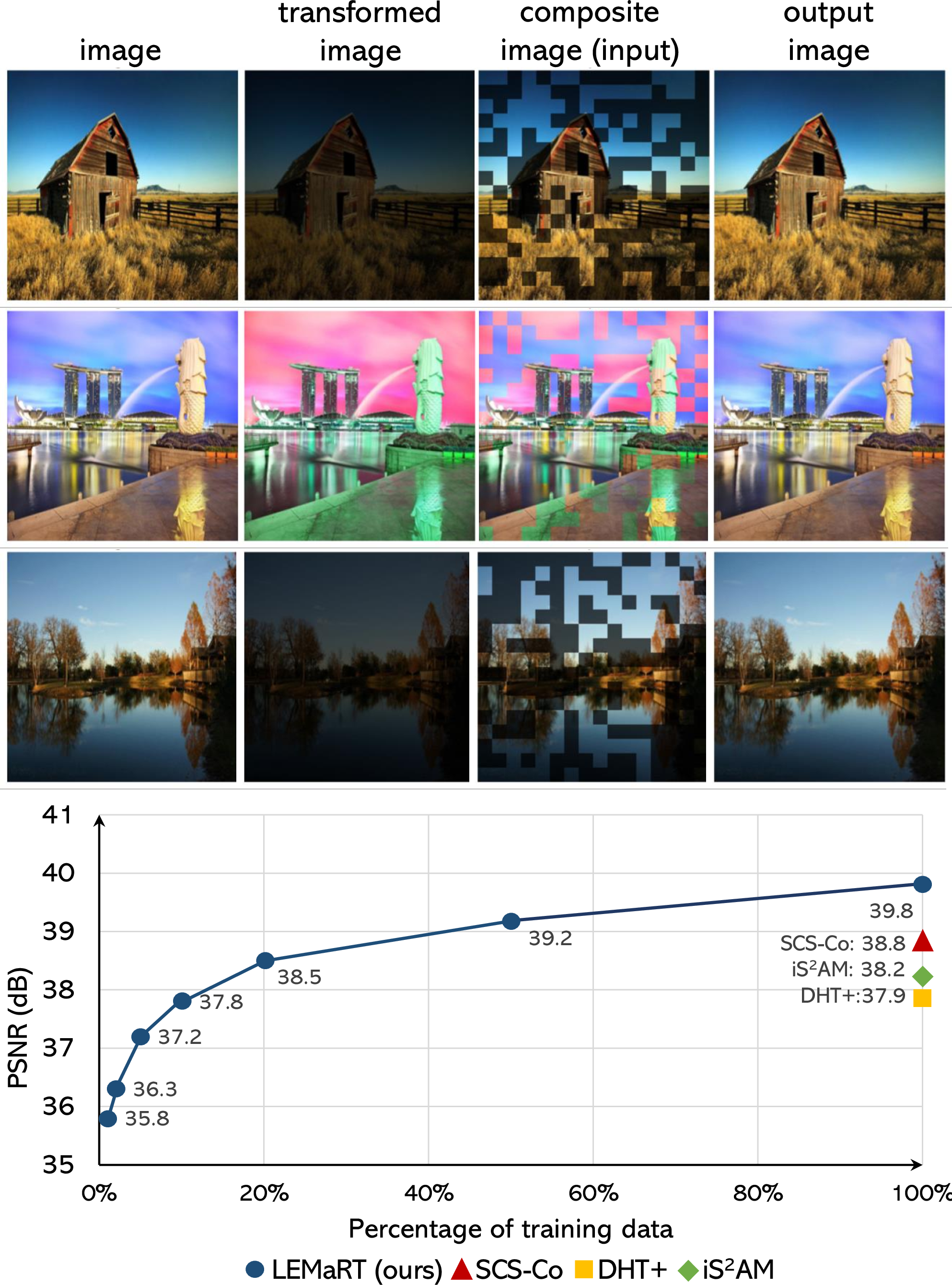
Inspired by the impressive performance leap achieved by pre-trained models [18], [19] on various downstream tasks, , image classification, object detection, image captioning, in this work, we introduce a novel self-supervised pre-training method to boost the performance of image harmonization models while being label-efficient, , consuming small amounts of fine-tuning data. The novelty of our technique lies in the use of foreground masking strategies and the perturbation of foreground visual attributes to self-generate training data without annotations. Hence, we name our pre-training method as Label-Efficient Masked Region Transform (LEMaRT). In the first step, LEMaRT proposes pseudo foreground regions in an image. Subsequently, it applies a set of transformations to perturb visual attributes of the foreground, including contrast, sharpness, blur and saturation. These transformations aim to mimic the appearance discrepancy between the foreground and the background. Using the transformed image, , image with the perturbed foreground, as the input, LEMaRT pre-trains image harmonization models to reconstruct the original image, as shown in the top half of Figure 1.
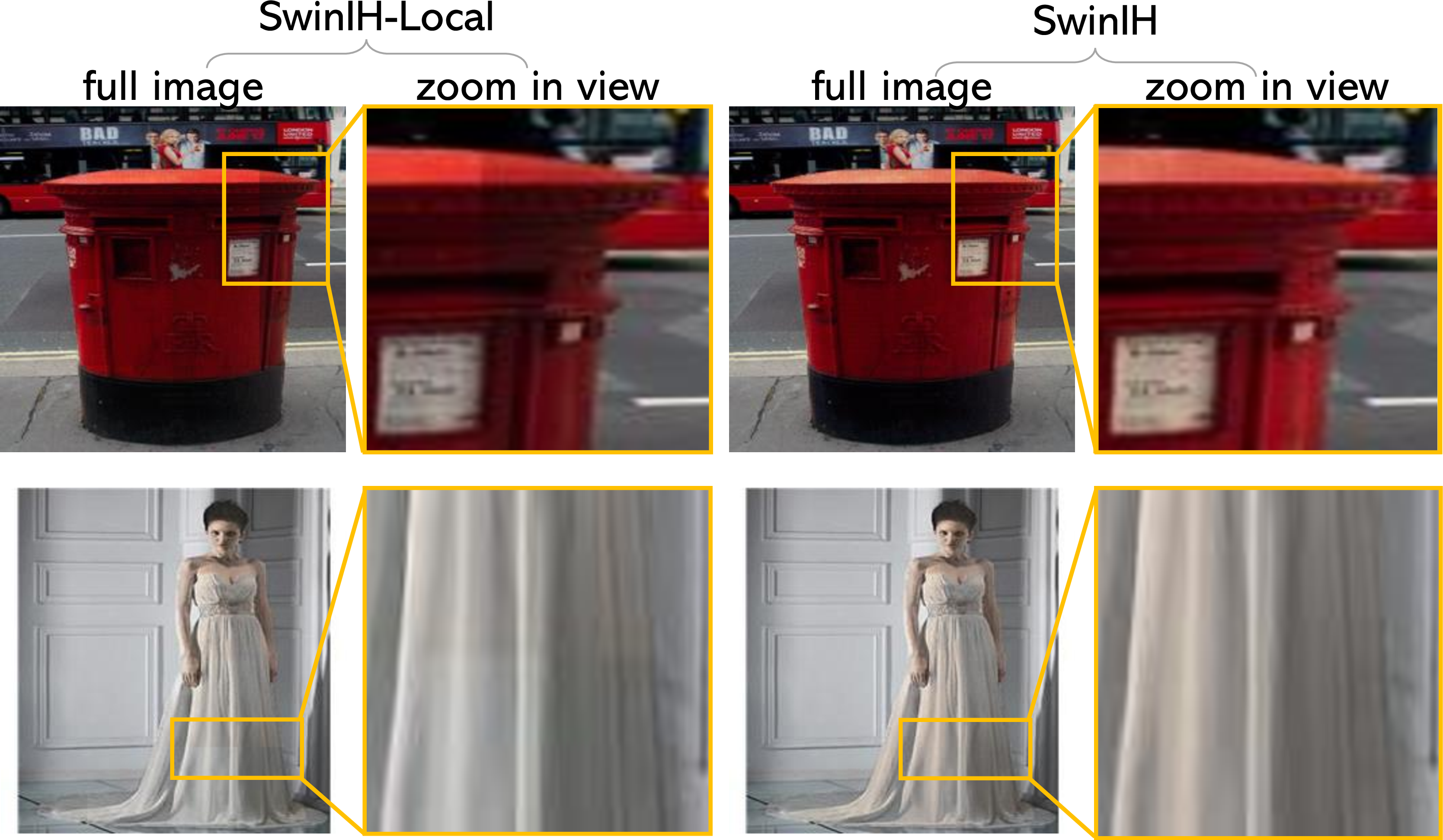
Subsequently, we design an image harmonization model based on Swin Transformer [1], namely SwinIH, which is short for Swin Image Harmonization. We build our model upon Swin Transformer instead of the ViT model [20] mainly due to the efficiency gain offered by its local shifted window (Swin) attention. Similar to the design of the original Swin Transformer, we keep the local self-attention mechanism in all the Transformer blocks up except the last one, where we employ global self-attention. We introduce global self-attention into SwinIH to alleviate block boundary artifacts produced by the Swin Transformer model when it is directly trained for image harmonization.
We verify that LEMaRT consistently improves the performance of models with a range of vision Transformer and CNN architectures compared to training only on the target dataset, , iHarmony4. When we pre-train our SwinIH model on MS-COCO dataset with LEMaRT and then fine-tune it on iHarmony4 [2], it outperforms the state of the art [3] by \(0.4\) dB while using only \(\textit{50}\%\) of the samples from iHarmony4 for fine-tuning, and by \(1.0\) dB when using all the samples (see the plot in the bottom half of Figure 1).
The key contributions of our work are summarized below.
\(\bullet\) We introduce Label-Efficient Masked Region Transform (LEMaRT), a novel pre-training method for image harmonization, which is able to leverage large-scale unannotated image datasets.
\(\bullet\) We design SwinIH, an image harmonization model based on the Swin Transformer architecture [1].
\(\bullet\) LEMaRT (SwinIH) establishes new state of the art on iHarmony4 dataset, while consuming significantly less amount of training data. LEMaRT also boosts the performance of models with various network architectures.
2 Related Work↩︎
a. Image Harmonization: Most early works extract and match low-level color statistics of the foreground and its surrounding background. These works rely on color histograms [11], multi-level pyramid representations [13], color clusters [12], etc. The limited representation power of low-level features negatively affects their performance.
More recent works [2], [17] have constructed datasets at a reasonable scale to advance learning-based methods. Numerous supervised deep learning-based image harmonization models have been trained on these datasets [16], [21]–[23]. Tsai [24] combine image harmonization and semantic segmentation under a multi-task setting. S\(^2\)AM [21] proposes to predict a foreground mask and to adjust the appearance of foreground with spatial-separated attention. RainNet [22] transfers statistics of instance normalization layers from the background to the foreground. In addition, generative models have also been trained for image harmonization [2], [25], [26].
Some state of the art (SOTA) methods formulate image harmonization as a style transfer problem. These methods learn a domain representation of the foreground and background with contrastive learning [27] or by maximizing mutual information between the foreground and background [28]. More recently, Hang [3] have advanced state of the art results by adding background and foreground style consistency constraints and dynamically sampling negative examples within a contrastive learning paradigm. Using only a reconstruction loss during pre-training and fine-tuning, our method is able to outperform [3] with a much simpler training set up.
b. Transfer Learning: Transfer learning is a well-known and effective technique for adapting a pre-trained model to a downstream task, especially with limited training data [29]–[31]. Recent advances in foundation models [18], [32]–[37] have resulted in models that can be adapted to a wide range of downstream tasks. Sofiiuk [38] propose an image harmonization model which takes visual features extracted from a pre-trained segmentation model as an auxiliary input. Instead of leveraging a pre-trained segmentation model for feature extraction, we specifically pre-train a model for image harmonization. We opt for this direction based on the hypothesis that pre-training for the same target task results in better performance than pre-training for a different task. Inspired by [29], our LEMaRT method is more suitable for image harmonization than [29] because LEMaRT creates training samples by applying transformations to the foreground rather than masking the foreground, which makes the pre-training task closer to image harmonization. In addition, [29] introduces an asymmetric encoder-decoder architecture, while our SwinIH model is specifically designed for image harmonization and does not have an explicit encoder or a decoder.
3 Method↩︎
3.1 Problem Formulation↩︎
The goal of image harmonization is to synthesize photo-realistic images by extracting and transferring foreground regions from an image \(\mathbf{I}_1\), specified by a binary mask \(\mathbf{M}\), to another (background) image \(\mathbf{I}_2\). Let \(\mathbf{I}_{c} = \mathbf{M} \odot \mathbf{I}_1 \oplus (1 - \mathbf{M}) \odot \mathbf{I}_2\) be the composite image generated by a direct copy and paste of the foreground region from \(\mathbf{I}_1\) on top of \(\mathbf{I}_2\). The operators \(\odot\) and \(\oplus\) denote element-wise multiplication and addition, respectively. Subsequently, an image harmonization function \(f(\cdot)\) transforms the composite image \(\mathbf{I}_{c}\) into a harmonized image \(\hat{\mathbf{I}} = f(\mathbf{I}_{c})\), such that the latter is photo-realistic. Deep learning-based image harmonization methods implement this function as a neural network \(f_\theta(\cdot)\) with parameters denoted by \(\mathbf{\theta}\). Our goal is to learn \(\mathbf{\theta}\) via self-supervised pre-training, so that the function \(f_{\mathbf{\theta}}(\cdot)\) can generate photo-realistic images.

3.2 Online Pre-training Data Generation↩︎
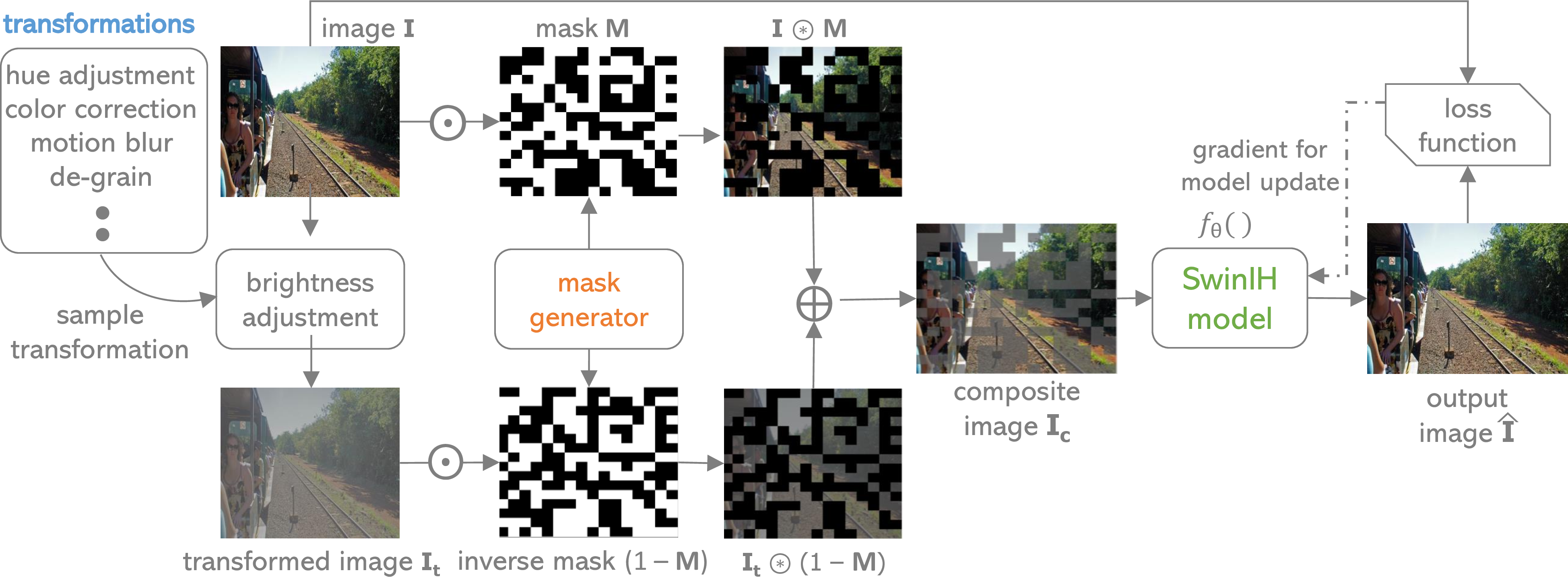
We first introduce our data generation and pre-training pipeline, , LEMaRT that generates the input and the ground truth for the pre-training process without relying on any manual annotations. As shown in Figure 2, LEMaRT applies a set of random transformations such as hue, contrast, brightness adjustment and defocus blur to perturb the original image \(\mathbf{I}\). The generated image is referred to as the transformed image \(\mathbf{I}_t\). The random transformations are designed to mimic different kinds of visual mismatches between a foreground region and a background image. In addition, LEMaRT employs a mask generation strategy to propose a foreground mask \(\mathbf{M}\) (please refer to \(\S\) 3.3 for more details). The mask and the set of transformations are generated on the fly for each input image \(\mathbf{I}\). With these ingredients, we generate a composite image \(\mathbf{I}_c\) from the original image \(\mathbf{I}\) and the transformed image \(\mathbf{I}_t\) as \(\mathbf{I}_{c} = \mathbf{M} \odot \mathbf{I}_t \oplus (1 - \mathbf{M}) \odot \mathbf{I}\). We note that the composite image \(\mathbf{I}_c\) is generated and fed into the network in an online fashion.
The goal of pre-training is to learn a harmonization function \(f_{\mathbf{\theta}}(\cdot)\) to resolve the mismatch of visual appearance between the foreground and the background of the composite image \(\mathbf{I}_{c}\). We formulate this task as the reconstruction of the original image \(\mathbf{I}\) from the composite image \(\mathbf{I}_{c}\). The original image \(\mathbf{I}\) serves as the supervision signal for the pre-training process under the assumption that visual elements of real images are in harmony. This formulation is applicable to a wide range of network architectures, e.g., SwinIH (see \(\S\) 3.4 for details), ViT [20] and CNN models [6], [39].
3.3 Mask Generation↩︎
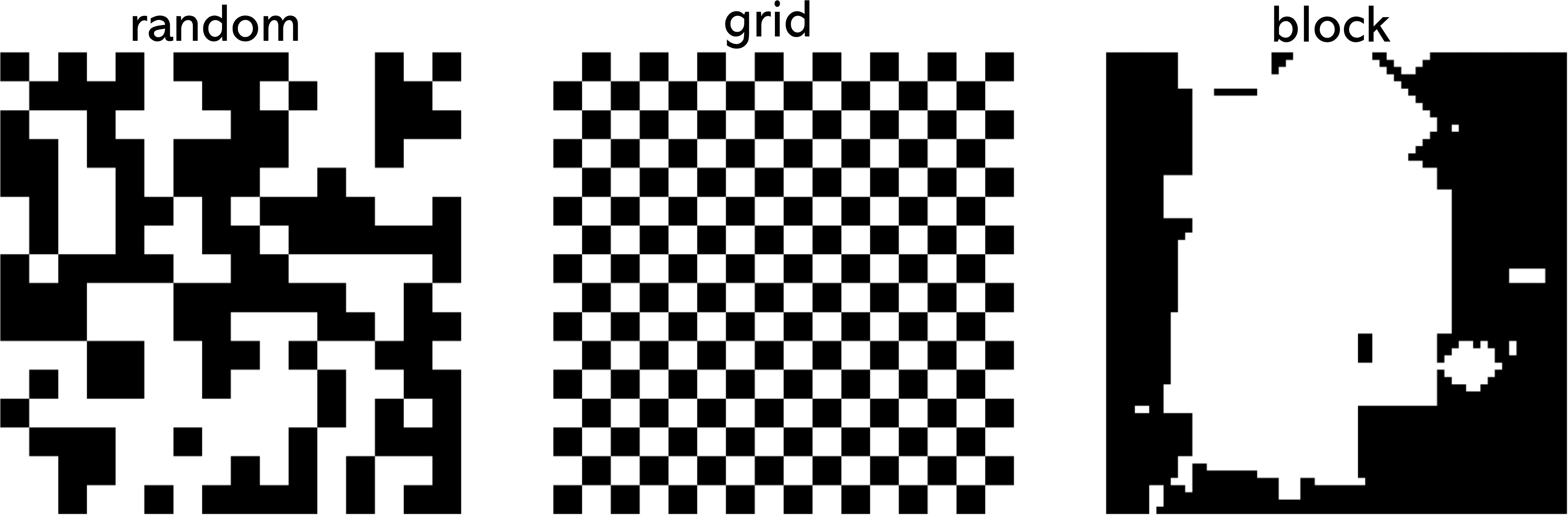
We now present three foreground mask generation strategies, which we refer to as random, grid and block.
\(\bullet\) random: as shown in Figure 4, this strategy first partitions an image into a regular pattern that consists of \(m \times m\) even patches (labelled by white pixels). It then generates a mask by randomly selecting a subset of the image patches.
\(\bullet\) grid: similar to random, this strategy first partitions an image into regular pattern of \(m \times m\) even patches. It then generates a fixed mask (same for all images) by selecting image patches following the pattern shown in Figure 4.
\(\bullet\) block: inspired by [40], we design a mask generation strategy that attempts to mimic the shape of objects. It generates a mask in an iterative manner. Each iteration has two steps, , (1) generating a rectangular region; (2) applying a random homography to the rectangular region to make the boundary of the region be composed of slanted lines. If the rectangular region is smaller than the size of the desired region to be masked, we generate a new region by executing the two steps once more and merge the newly generated region with previously generated regions (please refer to the supplementary materials for more details).
3.4 Network Architecture↩︎
Since the pre-training process is agnostic to network architecture, the only constraint for model design is that it needs to generate an output image of the same size as the input. To this end, we choose to implement our image harmonization model based on a Transformer architecture, due to the recent successes of vision transformer models in various tasks, including image harmonization [23], [41].
We choose to build our SwinIH model upon Swin attention blocks [1] due to its improved performance and efficiency over global attention layers used by ViT-style models [20], [23], [41]. Let \(H\) and \(W\) denote the height and width of an input image \(\mathbf{I}_{c}\) and \(N\) denote the size of an image patch. The length of the sequence of visual tokens is \(\frac{H \cdot W}{N^{2}}\). A global attention layer has a space and time complexity of \(\mathcal{O}(\frac{H^{2} \cdot W^{2}}{N^{2}})\). On the contrary, the space and time complexity of a Swin attention block is \(\mathcal{O}(\frac{H \cdot W \cdot K^{2}}{N^{2}})\), where the shifted window size \(K\) is smaller than \(H\) and \(W\).
The architecture of our SwinIH model is shown in Figure 3. It takes a four-channel image (a channel-wise concatenation of a composite image \(\mathbf{I}_c\) and a foreground mask \(\mathbf{M}\)) as input and generates an output image \(\hat{\mathbf{I}}\). Our SwinIH model is composed of three stages. The first two stages consist of three Swin attention blocks. The third stage has five Swin attention blocks and a global attention layer. We set the dimension of the patch embedding to \(128\) and double it at the end of the first two stages with linear projections.
Unlike Swin Transformer[1] which processes its input in a multi-scale manner1, we choose to preserve the original resolution of the input. As will be shown in \(\S\) [sec:exp-network], such a design choice is important as the information loss due to the reduced resolution hurts model accuracy.
3.5 Objective Function↩︎
We adopt the mean squared error (MSE) between the network’s output \(\hat{\mathbf{I}}\) and the original image \(\mathbf{I}\) as the objective function for pre-training. When we fine-tune the pre-trained network, we follow [38] and use a foreground-normalized MSE loss as the objective function.
| composite | DIH | S\(^2\)AM | DoveNet | BargNet | IntrHarm | RainNet | iS\(^2\)AM | DHT+ | SCS-Co | LEMaRT | ||
| dataset | metric | image | [24] | [21] | [2] | [27] | [16] | [22] | [38] | [41] | [3] | (SwinIH) |
| HCOCO | PSNR\(\uparrow\) | 33.9 | 34.7 | 35.5 | 35.8 | 37.0 | 37.2 | 37.1 | 39.2 | 39.2 | 39.9 | |
| MSE\(\downarrow\) | 69.4 | 51.9 | 41.1 | 36.7 | 24.8 | 24.9 | 29.5 | 16.5 | 15.0 | 13.6 | ||
| HAdobe | PSNR\(\uparrow\) | 28.2 | 32.3 | 33.8 | 34.3 | 35.3 | 35.2 | 36.2 | 38.1 | 37.2 | 38.3 | |
| MSE\(\downarrow\) | 345.5 | 92.7 | 63.4 | 52.3 | 39.9 | 43.0 | 43.4 | 21.9 | 36.8 | 21.0 | ||
| HFlickr | PSNR\(\uparrow\) | 28.3 | 29.6 | 30.0 | 30.2 | 31.3 | 31.3 | 31.6 | 33.6 | 33.6 | 34.2 | |
| MSE\(\downarrow\) | 264.4 | 163.4 | 143.5 | 133.1 | 97.3 | 105.1 | 110.6 | 69.7 | 67.9 | 55.8 | ||
| HD2N | PSNR\(\uparrow\) | 34.0 | 34.6 | 34.5 | 35.3 | 35.7 | 36.0 | 34.8 | 37.7 | 36.4 | 37.8 | |
| MSE\(\downarrow\) | 109.7 | 82.3 | 76.6 | 52.0 | 51.0 | 55.5 | 57.4 | 40.6 | 49.7 | 41.8 | ||
| all | PSNR | 31.6 | 33.4 | 34.3 | 34.8 | 35.9 | 35.9 | 36.1 | 38.2 | 37.9 | 38.8 | |
| MSE\(\downarrow\) | 172.5 | 76.8 | 59.7 | 52.3 | 37.8 | 38.7 | 40.3 | 24.4 | 27.9 | 21.3 | ||
4 Experiments↩︎
We evaluate our method by comparing its performance with other state-of-the-art (SOTA) methods and provide insights into our method through ablation studies. We adopt four metrics, , mean squared error (MSE), peak signal to noise ratio (PSNR), foreground mean squared error (fMSE )[2], and foreground peak signal to noise ratio (fPSNR) [2].
4.1 Datasets↩︎
Following previous works [2], [16], [27], we evaluate our method on iHarmony4 dataset [2]. For completeness, we also evaluate our method on RealHM dataset [17]. Unless otherwise stated, we pre-train our LEMaRT model on the set of 120K unlabeled images from the MS COCO dataset [42] and fine-tune on iHarmony4. There is no overlap between the images used for pre-training and the images used for fine-tuning and evaluation. Images in iHarmony4 either come from the set of labeled images in MS COCO, which is disjoint from the unlabeled images in MS COCO, or from other datasets. Following [2], [16], [24], [27], [38], we resize the input images and the ground truth images to \(256 \times 256\).
4.2 Implementation Details↩︎
We use an AdamW optimizer [43] both during pre-training and fine-tuning. We set \(\beta_{1}=0.9\), \(\beta_{2}=0.95\), \(\epsilon=1e^{-8}\) and weight decay to \(0.05\). The window size and the patch size of SwinIH are set to \(32\) and \(4\), respectively. We pre-train our model for \(30\) epochs with a batch size of \(192\) and a learning rate of \(2.7e^{-2}\). We then fine-tune the pre-trained model for \(120\) epochs with a learning rate of \(2.7e^{-3}\). A cosine annealing scheduler controls the change of learning rate. The minimum learning rate is set to \(0.0\). We adopt the random mask generation strategy and set mask ratio to \(50\)% during pre-training. This is the default setting for the experiments.
4.3 Comparison with SOTA Methods↩︎
a. On iHarmony4 Dataset
In Table 1, we present a comparison between the performance of our method, LEMaRT (SwinIH), and the performance of existing methods on iHarmony4. Overall, LEMaRT comprehensively outperforms existing methods across the two metrics (PSNR and MSE). Most notably, our method achieves a PSNR of \(39.8\) dB, which is \(1.0\) dB higher than the previous best method. The MSE of our method is \(16.8\), which is \(4.5\) lower (\(21.1\)% relative improvement) than the previous best method [3] 2.
We notice that our method, LEMaRT, consistently achieves better performance than SOTA methods [2], [3], [16], [21], [22], [24], [27], [38], [41] on three of the four subsets, , HCOCO, HAdobe and HFlickr of iHarmony4. Meanwhile, on the HD2N subset, the performance of our method is on par with SOTA methods. While our method yields higher PSNR, the MSE of our method is higher. We hypothesize that the domain of MS COCO, the dataset which we use to pre-train LEMaRT, is not closely aligned with that of HD2N. For example, mountains and buildings are the salient objects in most images in the HD2N subset. However, they do not often appear as the main objects in MS COCO images.
In Figure 5, we compare the harmonized images generated by three SOTA methods, i.e., RainNet, iS\(^2\)AM, DHT+, and our method, i.e., LEMaRT (SwinIH). We see that LEMaRT can generate photo-realistic images. Compared to other methods, LEMaRT is better at making color corrections, thanks to the pre-training process during which LEMaRT learns the distribution of photo-realistic images.
b. On RealHM Dataset
In Table 2, we compare the performance of our method, LEMaRT, with multiple SOTA methods on RealHM dataset. We pre-train our model on 120K images from Open Images V6 [44] for 22 epochs and then fine-tune our model on iHarmony4 for \(1\) epoch with a learning rate of \(5.3e^{-3}\). We see that LEMaRT comfortably outperforms DoveNet [2] and S\(^{2}\)AM [21], and achieves comparable results to SSH [17]. A comparison of the harmonized images generated by our LEMaRT method and existing methods can be found in the supplementary materials.
| method | DoveNet[2] | S\(^{2}\)AM[21] | SSH[17] | LEMaRT |
|---|---|---|---|---|
| MSE \(\downarrow\) | 214.1 | 283.3 | 206.9 | 206.1 |
| PSNR \(\uparrow\) | 27.4 | 26.8 | 27.9 | 27.6 |
| SwinIH | ViT[20] | ResNet[45] | HRNet[39] | HT+[41] | |||||||
| dataset | metric | w/o | w/ | w/o | w/ | w/o | w/ | w/o | w/ | w/o | w/ |
| all | PSNR\(\uparrow\) | 37.0 | 39.0 | 35.7 | 38.4 | 34.6 | 36.3 | 33.2 | 35.3 | 37.7 | 38.9 |
| MSE\(\downarrow\) | 35.5 | 20.9 | 48.2 | 24.1 | 64.4 | 44.2 | 78.5 | 48.4 | 31.4 | 22.3 | |
| fPSNR\(\uparrow\) | 24.5 | 26.6 | 23.1 | 25.9 | 21.9 | 23.4 | 20.6 | 22.7 | 25.1 | 26.3 | |
| fMSE\(\downarrow\) | 386.6 | 250.0 | 499.9 | 282.6 | 645.3 | 459.9 | 811.9 | 510.6 | 342.6 | 266.5 | |
4.4 Ablation Studies↩︎
We conduct ablation studies to gain insights into various aspects of our method. These aspects include the generalization ability of our LEMaRT method across different network architectures, its efficiency in terms of data and annotation consumption, the design choices of our SwinIH model, and the sensitivity of its performance to the mask generation strategy and the mask size.
a. Generalization Across Network Architectures
The goal of the first ablation study is to understand the effectiveness of the proposed pre-training method, i.e., LEMaRT, on various network architectures, including vision Transformers and convolutional neural networks (CNNs). Specifically, we adopt five different networks, i.e., SwinIH, ViT [20], ResNet [45], HRNet [39] and HT+ [41]. SwinIH refers to our model introduced in \(\S\) 3.4. ViT refers to the vision Transformer model that adopts global attention. ResNet is a variant of the ResNet generator introduced in pix2pixHD [45]. We remove the down sampling operators to make it suitable for image harmonization. We re-implement HT+ [41], a ViT-style Transformer model designed for image harmonization. Our implementation has comparable results (\(0.3\) dB higher PSNR, and \(0.9\) higher MSE) with those reported in [41]. We compare the performance of the five networks when they are trained on iHarmony4 from scratch (w/o columns in Table 3), and when they are fine-tuned after being pre-trained with LEMaRT (w/ columns). We train (or fine-tune) SwinIH, ViT, ResNet and HRNet on iHarmony4 for \(30\) epochs, and HT+ for \(120\) epochs to be consistent with the results reported in [41]. Other settings are kept the same as the default setting.
As shown in Table 3, pre-training on MS COCO with LEMaRT significantly improves performance of the models under study over training from scratch on iHarmony4. Specifically, the performance boost ranges from \(1.2\) to \(2.7\) dB in terms of PSNR and \(1.2\) to \(2.8\) dB in terms of fPSNR. In particular, LEMaRT improves the PSNR of our SwinIH model by \(2.0\) dB and its MSE by \(14.6\). Moreover, LEMaRT is effective not only for models adapted from other vision tasks, but also for those specifically designed for image harmonization, such as HT+ [41].
![Figure 5: Qualitative comparison between our method, LEMaRT (SwinIH), and three SOTA methods (RainNet[22], iS^2AM[38], DHT+[41]) on the iHarmony4 dataset. Compared to other methods, LEMaRT is better at color correction, thanks to the pre-training process during which LEMaRT learns the distribution of photo-realistic images.](/article/2304.13166/figures/qualitative3.png "fig:")
b. Data Efficiency
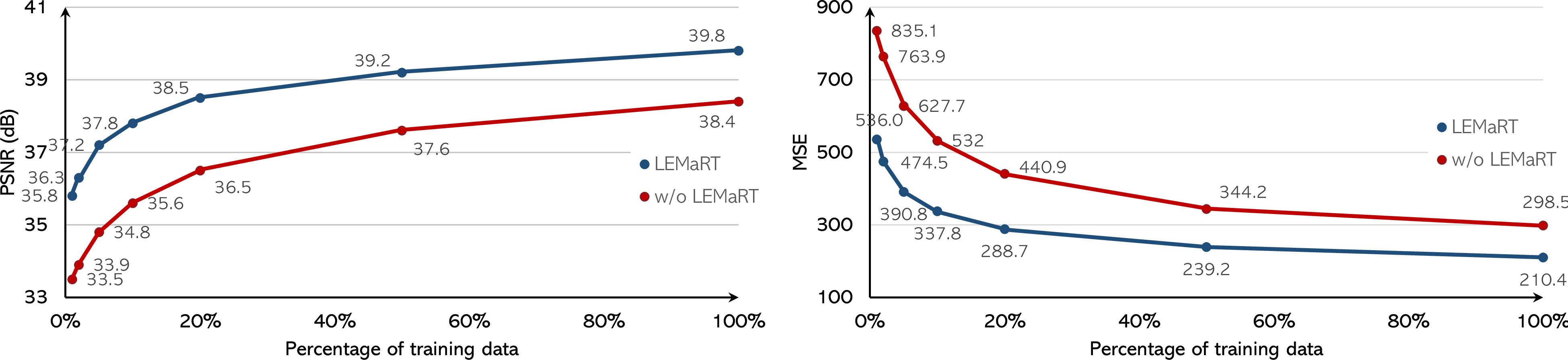
Next, we evaluate the effectiveness of LEMaRT with respect to the amount of fine-tuning data. As before, we pre-train our SwinIH model in two settings: training from scratch on iHarmony4 only and pre-training followed by fine-tuning. For both settings, we vary the amount of fine-tuning data by uniformly sampling between \(1\)% and \(100\)% of the iHarmony4 training set.
The results in Figure 6 are consistent with the previous section, in the sense that pre-training improves image harmonization accuracy by a large margin (up to \(2.4\) dB in terms of PSNR and \(299.1\) in terms of MSE) regardless of the amount of fine-tuning data. More importantly, the LEMaRT pre-training scheme is more beneficial to the low data regime than the high data regime. For example, when using no more than \(10\)% of the fine-tuning data, the performance boost attributed to pre-training ranges between \(2.3\) and \(2.4\) dB, whereas the improvement at \(100\)% of fine-tuning data declines to \(1.4\) dB. We observe a similar trend in the MSE measure, where the MSE improvement drops from around \(300.0\) at \(1\)% of iHarmony4 training data to less than \(90.0\) when using the full training set.
c. Model Design Choices
In this experiment, we pay attention to two design choices of our SwinIH model. The first choice is to maintain the input resolution across all the transformer blocks or to adopt a bottleneck layer similar to encoder-decoder models. The second choice is whether to use efficient local attention, , Swin attention, across all the blocks or to use global attention as well. This choice stems from a visual observation that the Swin attention occasionally induces block-shaped visual artifacts in harmonized images, as shown in Figure 7. Therefore, it prompts the necessity to modify model architecture to maintain a balance between efficiency and visual quality.
To gain insights into these aspects, we compare SwinIH, its two variants, , SwinIH-MS, SwinIH-Local, and Swin Transformer (Swin-T) [1]. SwinIH is introduced in \(\S\) 3.4. SwinIH-MS differs from SwinIH in that it first reduces and then enlarges the resolution of feature maps at deeper layers. SwinIH-Local replaces the global attention layer of SwinIH with a Swin attention block. As discussed in \(\S\) 3.4, Swin-T is composed of Swin attention blocks and uses a Patch Merging layer to reduce the spatial size of feature maps. We add a Patch Splitting layer (does the opposite of a Patch Merging layer) to enlarge the size of feature maps to make it suitable for image harmonization.
| model | |||||
| dataset | metric | SwinIH | MS | Local | Swin-T |
| all | PSNR\(\uparrow\) | 37.0 | 36.3 | 37.0 | 36.1 |
| MSE\(\downarrow\) | 35.5 | 41.3 | 35.1 | 47.0 | |
| fPSNR\(\uparrow\) | 24.5 | 23.7 | 24.5 | 23.2 | |
| fMSE\(\downarrow\) | 386.6 | 454.5 | 385.2 | 499.3 | |
As shown in Table 4, SwinIH significantly outperforms SwinIH-MS and Swin-T across all four metrics, , by \(0.7\) dB and \(0.9\) dB in terms of PSNR, and by \(5.8\) and \(11.5\) in terms of MSE, respectively. We hypothesize that the performance drop is caused by the information loss when the resolution of a feature map is reduced. The performance of SwinIH-Local and that of SwinIH are comparable in terms of PSNR and MSE. However, as shown in Figure 7, SwinIH produces results that are of higher visual quality. As shown in Figure 7, SwinIH-Local produces visible block boundaries. This is caused by the shifted window (Swin) attention, which prevents visual tokens at the border of each window to attend to its neighboring visual tokens in adjacent windows. SwinIH is able to remove these block-shaped artifacts. This demonstrates the benefit of using a combination of global and local attention. To maintain high computational and memory efficiency, we only employ it in the last layer of our model.
d. Mask Generation Strategy
| mask generation strategy | ||||
| dataset | metric | random | grid | block |
| all | PSNR\(\uparrow\) | 39.0 | 37.1 | 38.6 |
| MSE\(\downarrow\) | 20.9 | 33.5 | 23.2 | |
| fPSNR\(\uparrow\) | 26.6 | 24.5 | 26.1 | |
| fMSE\(\downarrow\) | 250.0 | 380.3 | 273.8 | |
Here we study the sensitivity of harmonization performance with respect to the mask generation strategy. To this end, we compare the three strategies discussed in \(\S\) 3.3, , random, grid and block. We measure the performance of our model after being pre-trained on MS COCO and fine-tuned on iHarmony4 for \(30\) epochs.
As seen in Table 5, the performance of grid strategy is worse that of the other two strategies. This result is expected, as the grid strategy can only transform image patches at specific locations. Therefore, it is not flexible for cases where there are multiple foreground regions or they cover an area larger than a grid cell. To our surprise, the random strategy achieves comparable performance to the block strategy, which is designed to mimic test cases. This result confirms that there is no need for a special mask generation algorithm that is tuned for the LEMaRT pre-training scheme. In other words, this simplifies the design and broadens the applicability of LEMaRT to new datasets.
e. Foreground Mask Size
| mask ratio | ||||
| dataset | metric | 30% | 50% | 70% |
| all | PSNR\(\uparrow\) | 38.8 | 39.0 | 39.0 |
| MSE\(\downarrow\) | 21.8 | 20.9 | 21.2 | |
| fPSNR\(\uparrow\) | 26.4 | 26.6 | 26.5 | |
| fMSE\(\downarrow\) | 255.0 | 250.0 | 250.5 | |
We examine the sensitivity of image harmonization results to the foreground mask size. Here, the foreground size is measured by the ratio of the foreground mask size to the image size. In this experiment, we fine-tune the pre-trained models for \(30\) epochs. In Table 6, we show the quantitative metrics at three different foreground mask ratios, 30%, 50% and 70%. We see that these metrics do not vary significantly between the three ratios. For example, fPSNR varies within a range with \(0.2\) dB width and fMSE varies within a range whose width is smaller than \(5.0\). This indicates that the size of generated foreground masks does not have significant impact on performance of pre-trained models.
5 Conclusion↩︎
In this work, we introduced Label-Efficient Masked Region Transform (LEMaRT), an effective technique of online data generation for self-supervised pre-training of image harmonization models. LEMaRT provides a simple, yet effective way to leverage large-scale unannotated datasets. In addition, we derived a Swin Transformer-based model that is more efficient than ViT-style Transformer networks for image harmonization. Extensive experiments on the iHarmony4 dataset validate the effectiveness of both our pre-training method and our model. We set a new state of the art for image harmonization, while showing that our pre-training method is much more label-efficient than the existing methods and is consistently applicable to a wide range of network architectures for image harmonization.
References↩︎
Swin Transformer[1] uses a Patch Merging layer to reduce the spatial size of its input by a factor of two at the end of each stage.↩︎
Our method also outperforms SOTA methods across the iHarmony4 dataset in terms of fPSNR and fMSE. For brevity, we omit them in Table 1 and include them in supplementary materials instead.↩︎