The Best of Both Worlds: Combining Model-based and Nonparametric Approaches for 3D Human Body Estimation
May 01, 2022
Abstract
Nonparametric based methods have recently shown promising results in reconstructing human bodies from monocular images while model-based methods can help correct these estimates and improve prediction. However, estimating model parameters from global image features may lead to noticeable misalignment between the estimated meshes and image evidence. To address this issue and leverage the best of both worlds, we propose a framework of three consecutive modules. A dense map prediction module explicitly establishes the dense UV correspondence between the image evidence and each part of the body model. The inverse kinematics module refines the key point prediction and generates a posed template mesh. Finally, a UV inpainting module relies on the corresponding feature, prediction and the posed template, and completes the predictions of occluded body shape. Our framework leverages the best of non-parametric and model-based methods and is also robust to partial occlusion. Experiments demonstrate that our framework outperforms existing 3D human estimation methods on multiple public benchmarks.
![Figure 1: From left to right: Original image our mesh prediction overlay and alternative views mesh visualization. Images are from 3DOH [1], and LSP [2] datasets. (Best viewed in Color)](/article/2205.00508/1st_img.png "fig:")
1 Introduction↩︎
The 3d estimation of the human body pose and shape from a monocular image is a fundamental task for various applications such as VR/AR, virtual try-on, metaverse and animations. It is challenging mostly due to the depth ambiguity and lack of evidence from single image. There are several ways to solve this ambiguity such as leveraging multi-view or video data to fuse image evidence from more images and infer occluded parts. For the case of single images, researchers used parametric models such as SMPL [3] to fit 2D image evidence [4] or use human pose prior [5]–[7] to penalize problematic human pose / mesh prediction in combination with modern deep learning techniques. However, these model-based methods are prone to produce corrupted results when severe occlusion happens.
Nonparametric methods use non-compressed representations like voxels [8], heatmaps [9] and joint location [10]–[12] as the target for modern deep learning. However, to estimate dense meshes they are computationaly expensive and consume lots of memory. They either use integral methods to estimate normalized joint location [9] or simplify meshes [12] to reduce the number of vertices. Without post-processing, these methods also generate qualitatively non-pleasing results. The dense correspondence methods [13]–[15], which are based on template SMPL human mesh surface and have been proven for various tasks.
Connecting nonparametric methods and model-based methods is hard due to the difficulty in localizing the corresponding feature. [9], [16], [17] utilize bounding boxes or keypoints location to find the related features to estimate necessary SMPL parameters. While [11], [18] learn the feature-parameter correspondence (attention) implicitly through neural networks. [14], [19] consider the correspondence between the mesh representation and pixel representation based on human surface mapping (UV coordinate system). However, they estimate the SMPL parameter through a light weight FC network and treat this simple optimization process as a post process. Their methods also do not convey the advantages of nonparametric methods such as robustness to occlusion.
To leverage the advantages from both worlds, we propose a 3d human body estimation framework that consists of three modules: Dense Map Prediction module (DMP), Inverse Kinematics module (IK) and UV Inpainting module (UVI). DMP explicitly predicts per-pixel human 3d joint location, 3d surface location in root relative coordinates, 3d displacement between the joint location and surface location, and also predicts UV coordinates which represent the human surface in a 2D grid. This module is robust to partial occlusion when predicting joint, as all the image evidence belongs to this part will contribute to the prediction explicitly. IK module connects the nonparametric prediction to model-based method. We first warp the DMP dense prediction to UV space and get the joint prediction based on the part-segmentation in UV space. Then we use a two-stage multi-layer perceptron, where the first stage inpaints and refines the joint prediction, while the second stage estimates SMPL parameters and eventually produces a posed mesh. With all the predictions in UV space from DMP and IK, UVI inpaints and refines the 3d body pose and mesh in UV space.
In summary, our contributions are three fold:
\(\bullet\) We propose a 3d body estimation framework from single image that seamlessly leverages the best of the both worlds (model-based and nonparametric).
\(\bullet\) The method is robust to occlusions and can self-correct wrong poses from Dense Map Prediction module.
\(\bullet\) We achieve state-of-the-art performance on H36M and 3DOH datasets.
2 Related Work↩︎
2.0.0.1 3D human shape estimation from monocular images
SMPL [3] has been widely used for 3D human mesh reconstruction. To boost its power in practice, a number of deep learning frameworks have been proposed by using SMPL as regression targets [4]–[6], [9], [14], [20]. [5] regresses SMPL parameters directly from input images by end-to-end training. Following this research direction, [9] add spherical Gaussian attention joint based on initial joint estimation, and the use the the attended feature to learn the vertices location. [4] combine learning and optimization[6] in the same framework but cannot handle occlusions. [14] uses the template UV mapping from SMPL and transforms 3d mesh reconstruction to decomposed UV estimation and position map inpainting problems. However, the way to get 3d human joint from SMPL mesh is based on the pre-trained joint regressor, which will induce intrinsic errors and usually does not generalize to other datasets.
2.0.0.2 3D human pose estimation from monocular images
Deep learning approaches have shown success in regressing 3D pose from a single image [8], [21]–[29]. Basically, most current models can be categorized into two frameworks. The first is to directly estimate 3D pose from images, based on volumetric representation [8], [21]. But these approaches may involve in high memory consumption and complex post-processing steps. Based on the explosive improvement in 2D pose estimation [23], another framework is to estimate 2D pose from images and then lift 2D pose to 3D pose [24], [25]. Since these approaches take 2D joint locations as input, 3D human pose estimation simply focuses on learning depth of each joint. This releases learning difficulty and leads to better 3D pose. However, there are few methods on systematically handling occlusion in the first framework while the second framework cannot recover information if the joint detector fails. Additionally, how to get human surfaces from the joint prediction remains a problem.
2.0.0.3 Inverse Kinematics
The inverse kinematics (IK) problem has been extensively studied in robotics [30], [31] and graphics [32] and its techniques have been used in 3d human pose estimation [18], [33]–[36]. Numerical solutions [30]–[32] rely on time-consuming iterative optimization. [33] uses temporal sequence to resolve IK ambiguity. [34] decomposes the IK rotation to the product of swing rotation and twist rotation and solve swing rotation analytically from predicted joint locations. Feed forward solution like [35], [36] propose BodyIKNet to regress SMPL [3] pose and shape parameters from 3d joint location, However, it leads to a sub-optimal solution when partial occlusion happens.

Figure 2: Our 3d body estimation framework consists of three part: Dense Map Prediction module (DMP), Inverse Kinematics and SMPL module (IK) and UV Inpainting Module (UVI)..
2.0.0.4 Occlusion
[37] presented a systematic study of various types of synthetic occlusions in 3D human pose estimation from a single RGB image. Since synthetic data can not fully depict the real occlusion, [38] learns from real data and uses grammar models with explicit occluding templates to reason about occluded people. To avoid specific design for occlusion patterns, [39] presents a method for modeling occlusion that aims at explicitly learning the appearance and statistics of occlusion patterns. They also synthesizes a large corpus of training data by compositing segmented objects at random locations over a base training image. [40] utilizes a cylinder model and confidence maps to filter out the occluded joints and uses flow warped joint in the same video to approximate the missing joints. [41] integrates depth information about occluded objects into 3D pose estimation. To provide full-geometry information to handle occlusion scenarios, [26] and [42] provide 3d scene geometry as multi-layer depth maps or signed distance fields into the inference stage. [43] proposes a simple but effeive self-training framework to adapt the model to highly occluded observations. To fully utilize the holistic human body model (e.g. SMPL [3]), [1] represents the target SMPL human mesh as UV location map and converts the full-body human estimation as an image inpainting problem. However, these frameworks either rely on nonparametric estimation or pure model-based regression, how to leverage the best of both worlds seamlessly remain an unexplored problem.
3 Method↩︎
As shown in Fig 2, our framework consists of three consecutive modules, including a dense map prediction module (DMP), which extract dense semantic maps (e.g. 3d joint location, surface location and their displacements) and correspondence UV position, an inverse kinematics and SMPL module (IK), which inpaint 3d joint location and estimate the smpl parameters, as well as a UV map inpainting module, which estimate the final joint location and mesh location in UV space.
3.1 Dense Map Prediction Module↩︎
Our dense map prediction module is an encoder-decoder architecture and is used to extract the IUV images \(M_i\), as well as dense semantic maps including dense joint map \(M_j\), dense location map \(M_l\) and dense displacement maps \(M_d\). They are further illustrated in Fig 3. \(M_i\) is generated from the continuous UV map from [14], it is continuous in both image space and UV space, thus, easier to learn compared with original UV map [3]. It is used to convert the dense local features as well as these semantic maps to UV space. For location map \(M_l\), it represents the position of each vertices from the SMPL human mesh surface in root-relative coordinates. To construct \(M_l\) groundtruth, we first use the SMPL model, SMPL parameters and camera parameters to generate the vertices location in root-relative coordinate, and generate the full UV space location map \(UV_l\) using barycentric interpolation (The mesh faces correspondence is defined by [14]). After that we use the \(M_i\) to fetch values from \(UV_l\) to get the dense location map in image space. For the generation of dense joint map \(M_j\), we first rely on T-pose SMPL mesh and assign each vertex to the nearest joints (14 LSP joints setting), after that we use barycentric interpolation to get the UV space assignment, and further refine the assignment by make it symmetric in UV space (e.g. left hip and right hip has symmetric shape in UV space, as illustrated in Fig 4). We term the part assignment in UV space as \(A_{uv}\) . After setting the assignment in UV space, we use the \(M_i\) to query values from \(UV_j\) to get the dense joint map in image space. \(UV_j\) stores the root-relative joint location. We define displacement as the residual between vertex location and the assigned joint location, thus \(UV_d = UV_l - UV_j\) and \(M_d = M_l - M_j\). As our human are left-right symmetric (e.g. left hand has symmetric shape with right hand and the size and the distance between joint and surface is almost the same.), the magnitude of left part and right part of \(UV_d\) should be the same.
These semantic maps are aligned with the human in the images. Thus we are able to train a encoder-decoder network to estimate directly from image space. Dense image space joint prediction shares the similar flavor with [44], [45].
The objective for the dense map prediction module is
\[{\ell_{DMP}} = {\ell_{M_i}} + {\ell_{M_l}} + {\ell_{M_j}} + {\ell_{M_d}} \label{eqn:DMP}\tag{1}\]
\(\ell_{M_i}\) is composed of two parts: a binary mask loss \(\ell_{M_ib}\) of human body, which distinguishes pixels from those at the background, and the human pixels. The loss function of \(\ell_{M_ib}\) is binary cross entropy loss. our CNN further outputs the UV coordinates and uses L1 loss \(\ell_{M_{iuv}}\) .
\[{\ell_{M_i}} = {\ell_{M_{ib}}} + {\ell_{M_{iuv}}} \label{eqn:mi}\tag{2}\]
For \(\ell_{M_l}\), \(\ell_{M_j}\) and \(\ell_{M_d}\), we use L1 loss to directly regress the real value. As these values are already in root-relative coordinate and in unit meters, thus their data range is \(-1\) to \(+1\), we do not further normalize them.
Our dense map prediction module not only predicts these semantic maps, but also extracts both global feature to estimate camera parameter and local feature for the UV impainting module.
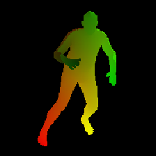
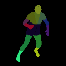
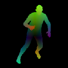
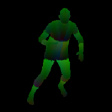
Figure 3: Semantic maps aligned with image space. From left to right: IUV image \(M_{i}\), Dense jointmap \(M_{j}\), dense location map \(M_{l}\) and dense displacement map \(M_{d}\). (Best viewed in Color).

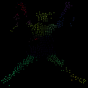

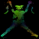
Figure 4: Warped Images in UV space based on IUV images \(M_i\). From left to right: Part segmentation in UV space \(A_{uv}\), UV space jointmap \(UV_{j}\), UV space location map \(UV_{l}\) and UV space displacement map \(UV_{d}\). (Best viewed in Color).

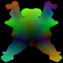
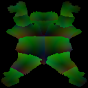
Figure 5: Full groundtruth in UV space. From left to right: UV space jointmap \(UV_{j}\), UV space location map \(UV_{l}\) and UV space displacement map \(UV_{d}\). (Best viewed in Color).
3.2 Inverse Kinematics Module↩︎
3.2.0.1 Estimate Joint Location from DMP
After warping the semantic maps (\(M_l,M_j,M_d\)) from image space to uv space, we get the incomplete uv joint map \(UV_j\). Based on the uv space joint assignment \(A_{uv}\) (as shown in Fig 4), we aggregate the dense prediction \(UV_j\) for each joint and average them if they are not fully occluded. Thus we have a coarse prediction for each joint \(J_{initial}\).
3.2.0.2 Joint Inpaint and Refine Module
Even though each human pixel contributes to joint prediction, there are still cases that some joints have no assigned vertex/pixel available from the image evidence. Thus we propose the joint inpainting module to inpaint these missing joints. This network is pretty flexible and can be MLP [24], GCN [25] or even modern transformers [46]. For the ease of implementation we use simple multi-layer perceptron. Our joint inpainting net is inspired by [24], which is simple, deep and a fully-connected network with six linear layer with 256 output features. It includes dropout after every fully connected layer, batch-normalization and residual connections. The model contains approximately 400k training parameters. The goal of this network is not only to inpaint the joints but also to refine the joints prediction that is not occluded. It takes the \(J_{initial}\) as input and the output of the network is the joint in root-relative coordinates \(J_{refine}\). We use L1 loss \(L_{ji}\) to train joint inpaint and refine module. The structure of the joint inpainting and refine module is shown in Fig 6.
3.2.0.3 Inverse Kinematics Module
After getting the sparse 3d human keypoints. We want to repose the template SMPL meshes based on the predicted joints location. To solve this problem we leverage inverse kinematics (IK). Typically, the IK task is tackled with iterative optimization methods [30]–[32], which requires a good initialization, more time and case-by-case optimization method. Here we propose a global inverse kinematics neural network GIK-Net. This network is constructed by the basic fully connected neural network module with residual connection, batch normalization and relu activation similar to [24]. In particular, GIK-Net takes the refined keypoint coordinates \(J_{refine}\) in root-relative space and outputs joint rotations \(\theta\) and \(\beta\) which serve as the input for SMPL layer. As we also use the Mocap dataset (AMASS [47], SPIN[4] and AIST++ [48]), our GIK-Net can implicitly learn the realistic distribution of human kinematics rotation and human shape. The use of the additional Mocap dataset serves the same purpose as the factorized adversarial prior [5], variational human pose prior [6] and motion discriminator [7]. We use L1 loss \(L_{\theta}\) and \(L_{\beta}\) to train GIK-Net. The structure of GIK-Net is shown in Fig 6.
3.2.0.4 SMPL revisits and Reposing Module
SMPL [3] represents the body pose and shape by pose \(\theta\in R^{72}\) and shape \(\beta\in R^{10}\) parameter. Here we use the gender-neural shape model following previous work [4], [5], [18]. Given these parameters, the SMPL module is a differentiable function that outputs a posed 3D mesh \(M(\theta,\beta) \in R^{6890 \times 3}\). The 3D joint locations \(J_{3D} = WM \in R^{J \times 3}\), while J are computed with a pretrained linear regressor \(W\). After getting the \(\theta\) and \(\beta\) from the GIK-Net we send them to SMPL layer to get the body mesh prediction.
We also augment the joints input for GIK-Net from Mocap dataset with guassian noise and random synthetic occlusion (30%). The augmentation helps our GIK-Net generalize to more realistic noisy input. We use L1 loss \(L_{vi}\) to train the mesh prediction from SMPL module.
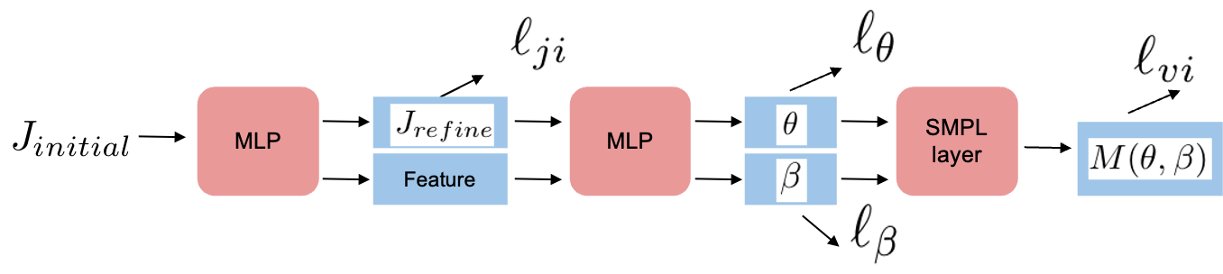
The objective for the inverse kinematics and smpl module is
\[{\ell_{IK}} = {\ell_{\theta}} + {\ell_{\beta}} + {\ell_{ji}} + {\ell_{vi}} \label{eqn:IK}\tag{3}\]
3.3 UV Inpainting Module↩︎
The goal of UV inpainting module is to regress 3d joint and mesh location directly based on the feature / semantic output (\(UV_l,UV_j,UV_d\)) from DMP and semantic output (\(UV_l,UV_j,UV_d\)) from IK.
3.3.0.1 Inevitable Fitting Error introduced by SMPL model and Joint regressor
The advantage of directly regressing joint/mesh location over model-based method is that model-based method will introduce intrinsic fitting error. Specifically, we use the SMPL layer, groundtruth SMPL parameters (from Mosh), and the joint-regressor [4] to obtain fitted joint for the whole Human3.6M dataset. We get average fitting error as 24.1 mm (MPJPE) when compared with the Human3.6M joint from Mocap system. It means that even we predict perfect SMPL mesh we still have about 24.1 mm fitting error. Thus we argue directly train and estimate joint location from UV space is a better alternative solution.
3.3.0.2 UV inpainting module
After getting the refined joint location \(J_{refine}\) from IK module, we distribute the refined joint location in UV space based on UV space joint assignment map \(A_{uv}\) and generate refine UV joint map \(UV_{jrefine}\). We also have the reposed template mesh and the corresponding reposed UV location map \(UV_{l}\) (through barycentric interpolation). Additionally, we have features \(UV_f\), location map \(UV_l\), joint map \(UV_j\) and displacement \(UV_d\) from DMP. We combine the best of both worlds ( DMP and IK) feature through aggregation and send it to our UV inpainting module. The UV inpainting module is a light UNet with skip connections. We can see the Fig 5 is the complete version of Fig 4 and serves as the groundtruth for the UV inpainting module.
For the training of the UV inpainting module, we have \[{\ell_{map}} = \| {\hat{UV}_{map}} - UV_{map} \|_{1} \label{eqn:map}\tag{4}\] Note the ‘map’ represents location map, joint map and displacement map in uv space. Addtionally, we have 3d joints and 2d joint loss based on the predicted camera parameter. Our camera parameters consist of scale and offset parameter to map the xy in \(J_{3d}\) to \(J_{2d}\). \[{\ell_{j3d}} = \| {\hat{J}_{3d}} - J_{3d} \|_{1} \label{eqn:j3d}\tag{5}\] \[{\ell_{j2d}} = \| {\hat{J}_{2d}} - J_{2d} \|_{1} \label{eqn:j2d}\tag{6}\] As we know, the distance between the human surface to the joints are left-right symmetric, thus we also apply symmetric loss on the magnitude of displacement. \[{\ell_{dismag}} = \| \|{\hat{UV}_{d}}\| - \|{\hat{UV}^{flip}_{d}}\| \|_{1} \label{eqn:displacementmagnitude}\tag{7}\]
To align the predicted mesh surface with image aligned IUV images \(M_i\), we also adopt consistent loss from [14]. It is enabled by the camera parameter predicted by our model (scaling and offset parameter).
The objective for the uv inpainting module is
\[{\ell_{UVI}} = {\ell_{dismag}} + {\ell_{j2d}} + {\ell_{j3d}} + {\ell_{map}} + {\ell_{con}} \label{eqn:UVI}\tag{8}\]
Thus we have all the losses as
\[{\ell_{all}} = {\ell_{DMP}} + {\ell_{IK}} + {\ell_{UVI}} \label{eqn:allloss}\tag{9}\]
3.3.0.3 Inference
We do inference of 3d joint location from \(UV_j\) and based on the uv assignment \(A_{uv}\) for each joint. We average all the prediction for the specific joints if this pixel prediction is valid. For human mesh prediction we use the barycentric interpolation from the UV space location map \(UV_l\).
3.4 Implementation Details↩︎
The proposed framework is trained on the ResNet-50 [49] backbone pre-trained on ImageNet. It takes a 224 \(\times\) 224 image as input, and input resolution for UVI is 64 \(\times\) 64 and the output resolution is 128 \(\times\) 128. We train three modules separately. We first train our DMP, and based on the output of DMP and Mocap data we train our IK; We finally fix and concat DMP and IK, and train UVI module. We apply synthetic occlusion [50] when train DMP. The training data is augmented with randomly scaling, rotation, flipping and RGB channel noise. We use the Adam optimizer. The training data for each module is illustrated in Table ¿tbl:table:traingset?.
4 Experiments↩︎
4.1 Dataset and Evaluation Metric↩︎
| Stages | Training Datasets |
|---|---|
| DMP | H36M, MPI-INF-3DHP, MPII, COCO, LSP |
| IK | H36M, MPI-INF-3DHP, AMASS, AIST++ |
| UVI | H36M, 3DOH |
4.1.0.1 Human3.6M
[51] is commonly used as the benchmark dataset for 3D human pose estimation, consisting of 3.6 millions of video frames captured in the controlled
environment. It has 11 subjects, 15 kinds of action sequences and 1.5 million training images with accurate 3D annotations. Similar to [5], we use MoSH to process
the marker data in the original dataset, and obtain the ground truth SMPL parameters to generate the groundtruth for \(UV_l\). For a fair comparison, we use 300K data in S1, S5, S6, S7, S8 for network training, and test in
S9, S11.
3DOH [1] utilize multi-view SMPLify-X [6] to get the 3d ground truth. The dataset is designed to have object occlusion for subjects. It contains 50,310 training images and 1,290 test images. It provides 2D, 3D annotations and SMPL parameters to generate meshes.
We use the test set for evaluation purposes and the training set to train the UVI module.
LSP [2] dataset is a 2D human pose estimation benchmark. In our work, we use the [52] SMPL parameter to render the \(M_{i}\) to train DMP module.
MPI-INF-3DHP [53] is a dataset captured with a multi-view setup mostly in indoor environments. No markers are used for the
capture, so 3D pose data tend to be less accurate compared to other datasets. We use the provided training set (subjects S1 to S8) for training. We use the it to train DMP and IK module.
Mocap dataset We use [47] AMASS, AIST++ [48] and SPIN [4] dataset to train our occlusion aware GIKNet.
Evaluation We evaluate our method on H36M [51] dataset and 3DOH [1] datasets. We report Procrustes-aligned mean per joint position error (MPJPE-PA) and mean per joint position error (MPJPE) in mm. For 3DOH we also report mean per vertex error (MPVE) in mm.

Figure 7: Different part segmentation choice in UV space. (Best viewed in Color).
| H36M | ||
|---|---|---|
| Method | MPJPE | MPJPE-PA |
| HMR [5] | 88.0 | 56.8 |
| DaNet [15] | 61.5 | 48.6 |
| HoloPose [16] | 60.3 | 46.5 |
| SPIN [4] | 62.5 | 41.1 |
| I2L [9] | 55.7 | 41.1 |
| DetNet [35] | 64.8 | 50.3 |
| PHMR [34] | - | 41.2 |
| DecoMR [14] | 60.5 | 39.3 |
| PyMaf [19] | 57.7 | 40.5 |
| Ours DMP-14 | 69.7 | 51.7 |
| Ours IK-14 | 67.3 | 50.6 |
| Ours UVI-14 | 54.7 | 38.4 |
| 3DOH | |||
|---|---|---|---|
| Method | MPJPE | MPJPE-PA | MPVE |
| SMPLify-X | - | 156.4 | 177.3 |
| OOH [13] | - | 58.5 | 63.3 |
| SPIN [4] | 104.3 | 68.3 | 113.4 |
| PyMAF[19] | 96.2 | - | 107.3 |
| HMR-EFT\(^{\star}\) [54] | 75.2 | 53.1 | - |
| PARE\(^{\star}\) [18] | 63.3 | 44.3 | - |
| Ours DMP-14 | 128.4 | 109.8 | - |
| Ours IK-14 | 112.9 | 80.8 | 133.5 |
| Ours UVI-14 | 58.3 | 44.6 | 72.3 |
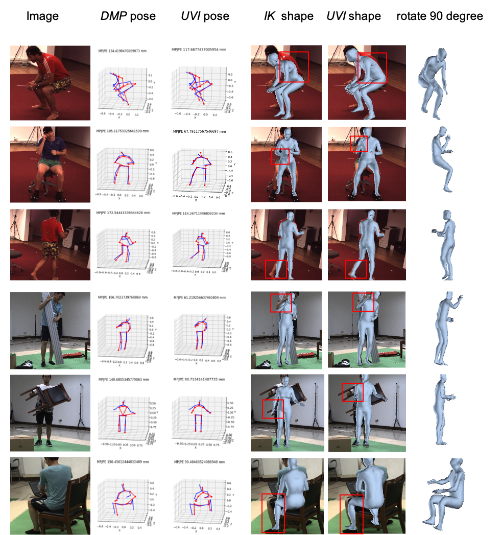
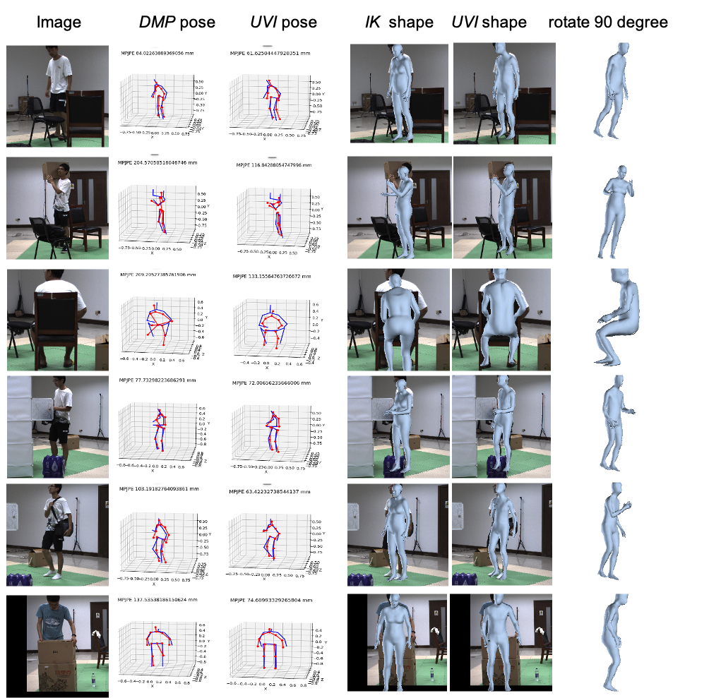
Figure 8: Pose and shape prediction from DMP module, IK module and UVI module. (Best viewed in Color).
4.2 Quantitative Results↩︎
4.2.0.1 Comparison with SOTA performance
We can see our final stage (UVI-14) in Table ¿tbl:table:h36m? achieve state-of-the-art performance on common H36M benchmark. Our SOTA performance demonstrates the usefulness of proposed combination of model-based and nonparametric approaches. In Table ¿tbl:table:3doh?, as our methods focus on both pose and mesh while [13] focus more on meshes, they achieve SOTA performance on 3DOH dataset; PARE [18] uses the EFT dataset [54] with improved groundtruth thus outperforms us on MPJPE-PA metric.
4.2.0.2 14 joints vs 24 joints setting
Another way to get 24 joints prediction from DMP is to have a 24 joints segmentation \(A_{uv}\) in UV space following SMPL setting. As shown in Fig 7 we define 14 joints setting and 24 joints setting. We run DMP-24 and DMP-14 and evaluate on the predicted \(J_{initial}\). We observe the error of DMP-24 is much higher than DMP-14 as in Table ¿tbl:table:3dohablstions?. The main reason is that over-segment of body parts may distribute less visible pixels to certain parts (feet, hand) and will lead to higher error.
4.2.0.3 Occlusion vs Non-occlusion
When computing the MPJPE for \(J_{initial}\), the results for visible parts (part with any pixel belong to them visible) and invisible parts differ a lot. We compare the DMP-14 and DMP-14-Nonoccluded in Table ¿tbl:table:3dohablstions?. We find visible parts with 87.3 mm MPJPE while the MPJPE counting invisible parts yield 128.4 mm. It tells us if the joints are visible, our DMP can predict relative good initial results. Thus, synthetic occlusion helps for our DMP module. When we remove the data augmentation techniques like synthetic occlusion [50], DMP-14 increase to 135.4 mm.
| 3DOH | |||
|---|---|---|---|
| Method | MPVE | MPJPE | PMPJPE |
| DMP-24 | - | 246.4 | 208.5 |
| DMP-14 w/o synthetic occlusion | - | 135.4 | 115.7 |
| DMP-14-Nonoccluded | - | 87.3 | 64.7 |
| DMP-14 | - | 128.4 | 109.8 |
| IK-14 w/o gaussian noise | 138.2 | 115.7 | 82.8 |
| IK-14 w/o random zero | 139.5 | 116.8 | 83.2 |
| IK-14 | 133.5 | 112.9 | 80.8 |
| UVI-14 w/o IK-14 | 82.9 | 69.4 | 58.1 |
| UVI-14 w/o DMP-14 | 80.1 | 67.8 | 55.1 |
| UVI-14 w/o \(\ell_{dismag}\) | 75.5 | 63.8 | 47.3 |
| UVI-14 | 72.3 | 58.3 | 44.6 |
4.2.0.4 GIK-Net data augmentations
We also try to remove the gaussian noise or random mask out joints data augmentation techniques for MOCAP data, which serve as input for the GIK-Net, to see how is the MPJPE varying. As shown in Table ¿tbl:table:3dohablstions?, IK-14 w/o gaussian noise and IK-14-w/o random zero yield larger error (2.8 mm and 3.9 mm ) compared with IK-14. It demonstrate these data augmentation makes the GIK-Net more robust to noise and helps generalize to real data input.
4.2.0.5 UVI ablations
As the magnitude of our \(UV_{d}\) should be symmetric, we introduce the magnitude error for \(UV_{d}\) and its flip version. We run a model without this \(\ell_{dismag}\) and observe there is 4.5 mm error increase in MPJPE metric. This is shown in Table ¿tbl:table:3dohablstions?.
4.2.0.6 Each stage performance
DMP module is a nonparametric method, while IK module is a model-based method relying on the output of DMP and then correct it. UVI module relies on both nonparametric output and model-based output, and predict the final body joint and mesh. Based on Table ¿tbl:table:3dohablstions?, DMP-14 estimate from raw images and gives inferior performance. IK-14 corrects the output from DMP-14 and reduce the error by 15.5 mm. UVI-14 relies on both IK-14 and DMP-14 and further reduce MPJPE to 58.3 mm. However, if any of the previous stage output is missing, MPJPE increase by 11.1 mm (w/o IK-14) or 8.5 mm (w/o DMP-14).
4.3 Qualitative Results↩︎
We present qualitative results in Fig 8 including the joints prediction from DMP, IK, UVI modules and mesh prediction from IK, UVI modules.
4.3.0.1 Limitations
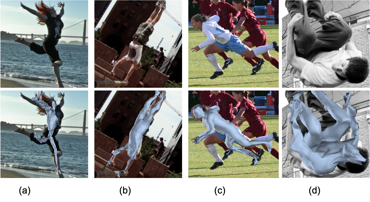
We also show failure cases in Fig 9. Typical failure cases can be attributed to challenging poses (a,b,d), and crowded scenarios (c).
5 Conclusion↩︎
We propose a framework that combine the best of both worlds (nonparametric and SMPL model-based method). It predicts the initial 3d body pose from DMP module, refine the predicted pose and repose the template SMPL meshes using IK module. Based on the nonparametric prediction from DMP module and model-based prediction from IK module, the UVI module inpaint and refine the prediction. To alleviate the intrinsic error introduced by joint regressor (fitting), we regress joint (\(UV_j\)) and mesh (\(UV_l\)) separately in different maps in UV space. We also introduce the magnitude loss \(\ell_{dismag}\) to enforce the symmetric property of human (\(UV_d\)). Our framework achieves state-of-the-art performance among 3D mesh-based methods on several public benchmarks. Future work can focus on extending the framework to the reconstruction of full body surfaces including hands and faces.
Appendix↩︎
6 Qualitative Results↩︎
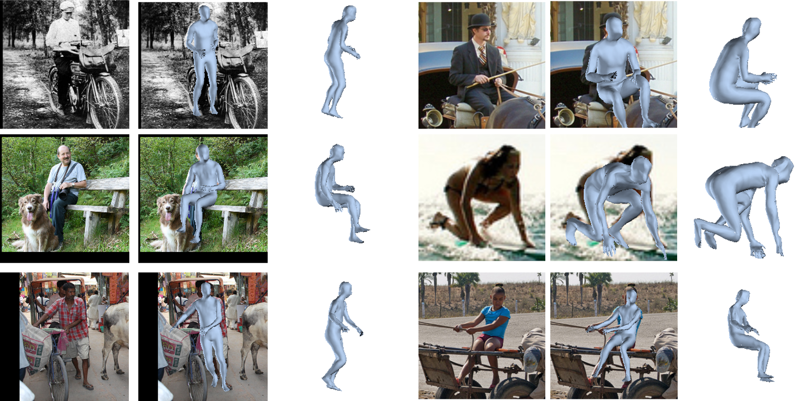
We show more qualitative results on COCO [55] in Fig 10, and 3DOH [1] in Fig 11.
7 Part Segmentation in UV Space↩︎
We first use the reference T-pose mesh and the LSP joint regressor provided by [4], [14] to get the T-pose 14 joint location. Then we calculate the joint-vertex euclidean distance and assign vertex to joint based on the smallest distance. After that, we use the barycentric interpolation (mapping between vertex triangle and UV space triangles) to get the UV space assignment probability (\(128 \times 128 \times 14\)). Following these operations, we use argmax to get the final assignment for each UV grid to the joint location.
8 Implementation Details↩︎
For AMASS [47] data, we only get SMPL-H [6] fitting instead of SMPL fitting data, however, SMPL-H does not included hands rotations as in SMPL. We sample random rotations from SPIN [4] fitting or the predictions from our DMP stages for its training data. For AIST++ [48], it does not included \(\beta\) parameters, we sample \(\beta\) from SPIN [4] fitting or the predictions from our DMP stages for its training data. We use the original rotation representation from SMPL [3] (axis-angle representation) for the fast training purpose.