CODEs: Chamfer Out-of-Distribution Examples against Overconfidence Issue
August 13, 2021
Abstract
Overconfident predictions on out-of-distribution (OOD) samples is a thorny issue for deep neural networks. The key to resolve the OOD overconfidence issue inherently is to build a subset of OOD samples and then suppress predictions on them. This paper proposes the Chamfer OOD examples (CODEs), whose distribution is close to that of in-distribution samples, and thus could be utilized to alleviate the OOD overconfidence issue effectively by suppressing predictions on them. To obtain CODEs, we first generate seed OOD examples via slicing&splicing operations on in-distribution samples from different categories, and then feed them to the Chamfer generative adversarial network for distribution transformation, without accessing to any extra data. Training with suppressing predictions on CODEs is validated to alleviate the OOD overconfidence issue largely without hurting classification accuracy, and outperform the state-of-the-art methods. Besides, we demonstrate CODEs are useful for improving OOD detection and classification.
In this paper, we define a novel set of effective OOD examples, whose distribution is close to that of in-distribution samples, and thus are more effective for alleviating the OOD overconfidence issue by suppressing predictions on them. To obtain effective OOD examples with training data only, we propose to first generate seed examples that are OOD via slicing&splicing operations on in-distribution samples from different categories, and then feed them into the Chamfer generative adversarial network for distribution transformation. Training with suppressing predictions on the generated Chamfer OOD examples (CODEs) are validated to alleviate the OOD overconfidence issue largely without hurting classification accuracy, and outperform the state-of-the-art methods. Besides, we demonstrate CODEs are useful for improving OOD detection and classification. Codes will be made public.
Specifically, we devise a chamfer generative adversarial net (Chamfer GAN), which converts seed adversarial examples to Chamfer OOD examples (CODEs)
utilize wasserstein and chamfer distance loss
To obtain CODEs, we adopt slicing&splicing operations on samples from different categories to generate seed adversarial examples firstly, and then feed them into a novel chamfer generative adversarial net (Chamfer GAN), which utilize wasserstein and chamfer distance loss to enforce CODEs to be hard. We validate that the overconfidence issue of DNNs on OOD samples could be significantly alleviated after adversarial training with CODEs. Besides, we demonstrate adversarial training with CODEs could improve classification.
close to the distribution of in-distribution data.
We hypothesis that CODEs close to the distribution of in-distribution data are more effective.
the number of OOD examples (OOD examples) can be infinitely many, adversarial training without sufficiently effective OOD examples could hardly work .
The number of OOD examples (OOD examples) can be infinitely many, making existing adversarial training approach without selection the most effective ones could hardly work.
In this paper, we hypothesis that OOD examples close to the distribution of in-distribution data are more effective.
whose effectiveness for improving adversarial robustness vary a lot. Without intentionally selection of the most effective ones, existing adversarial training approach could hardly work. In this paper, we hypothesis that OOD examples close to the distribution of in-distribution data are more effective for adversarial training to take effect.
However, existing adversarial training approach could hardly work without sufficiently effective OOD examples (OOD examples).
However, existing OOD examples (OOD examples) could bring unsatisfying strengthen effect after adversarial training.
an overwhelming number of easy examples and a small number of hard examples. Automatic selection of these hard examples can make training more effective and efficient
Since without any constraint against OOD, existing OOD examples (OOD examples) could bring unsatisfying strengthen effect after adversarial training.
However, existing OOD examples (OOD examples) could bring unsatisfying strengthen effect after adversarial training. By analogy with hard example mining, we hypothesize that OOD examples that are close to the distribution of in-distribution data are the “hard examples” for adversarial training to take effect.
In this paper, we propose Chamfer OOD examples (CODEs) which is a hard OOD examples. To obtain CODEs, we adopt slicing&splicing operations on samples from different categories to generate seed adversarial examples firstly, and then feed them into a novel chamfer generative adversarial net (Chamfer GAN), which utilize wasserstein and chamfer distance loss to enforce CODEs to be hard. We validate that the overconfidence issue of DNNs on OOD samples could be significantly alleviated after adversarial training with CODEs. Besides, we demonstrate adversarial training with CODEs could improve classification.
Alleviating the overconfidence issue on out-of-distribution (OOD) samples in the view of adversarial examples is promising. However, since current false positive adversarial examples (OOD examples) are unrestricted, adversarial training with them could hardly work. In this paper, we propose chamfer adversarial examples (CAEs), which is a kind of ‘hard’ OOD examples satisfying three key properties: false, adversarial to be positive and distribution-restricted, Specifically, we first generate seed adversarial examples by combining patches from images in different categories, and then refining their distribution distance to the training set by utilizing generative adversarial nets and chamfer distance loss. We validate the overconfidence issue of deep networks on OOD samples could be significantly alleviated after adversarial training with chamfer adversarial examples. Besides, we demonstrate adversarial training with chamfer adversarial examples could improve classification.
1 Introduction↩︎
Deep neural networks (DNNs) have obtained state-of-the-art performance in the classification problem [1]. Classification systems are generally designed for a static and closed world [2]. With the occurrence of new concepts in real world, current DNN classifiers will still attempt to make predictions. Since those classification systems are generally designed for a static and closed world [2], DNN classifiers will attempt to make predictions even with the occurrence of new concepts in real world. Unfortunately, those unexpected predictions are likely to be overconfident. Indeed, a growing body of evidences show that DNN classifiers suffer from the OOD overconfidence issue of being fooled easily to generate overconfident predictions on OOD samples [3], [4].
A widely adopted solution is to calibrate the outputs between in- and out-of-distribution samples to make them easy to detect [5], [6]. By this way, overconfident predictions on OOD samples could be rejected as long as identified by OOD detectors. While those approaches are significant steps towards reliable classification, the OOD overconfidence issue of DNN classifiers remains unsolved. Besides, as challenged by Lee et al. [7], the performance of OOD detection highly depends on DNN classifiers and they fail to work if the classifiers do not separate the predictive distribution well. This motivates us to resolve the OOD overconfidence issue inherently with enforcing DNN classifiers to make low-confident predictions on OOD samples.
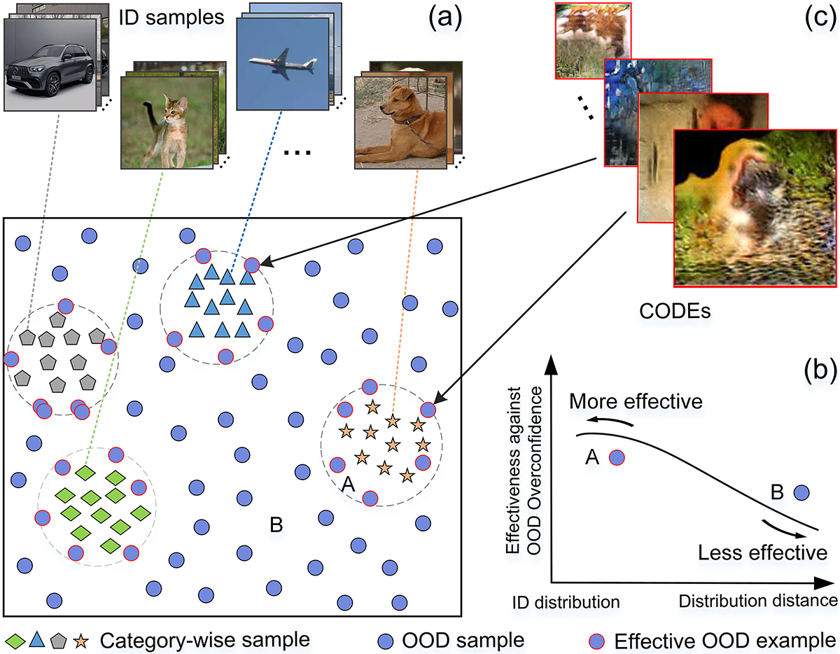
Since with infinite amount, the key to resolve the OOD overconfidence issue is to build a subset of OOD samples and then suppress predictions on them. Lee et al. [7] use a generative adversarial network [8] to model the subset which, however, requires to be tuned on the testing-distribution. Without synthesizing data from a carefully designed distribution, Hendrycks et al. [9] adopt an auxiliary dataset to simulate the subset. However, the optimal choice of such dataset remains an open question, challenges of data imbalance and computational complexity make it less efficient and practical [10]. In contrast, Hein et al. [11] simply adopt random noises and permuted images, and report promising results. It thus brings us to the main topic of this paper (see Fig. 1): can we get a subset of OOD samples that is more effective for alleviating the OOD overconfidence issue by suppressing predictions on them? Intuitively, suppressing a subset of OOD samples whose distribution is close to that of in-distribution (ID) samples, are expected to bring more benefits, since they are harder to be differentiated by DNNs to make low-confident predictions. Under this hypothesis, we propose to generate a subset of OOD samples whose distribution is close to that of ID samples, i.e., effective OOD examples.
In this paper, we propose the novel Chamfer OOD examples (CODEs), which is a kind of effective OOD examples. Besides, we devise a simple yet effective method to generate CODEs with training data only. Specifically, we first generate seed examples that is OOD by slicing&splicing operations, and then feed them into the Chamfer generative adversarial network (Chamfer GAN) for distribution transformation. Particularly, the Chamfer distance loss is intentionally imposed on Chamfer GAN to maintain the pixel-level statistic of seed examples, such that CODEs remain to be OOD. We validate the effectiveness of our approach that suppresses predictions on CODEs during training, and compare it with the state-of-the-art methods. Extensive experiments show that the OOD overconfidence issue will be largely alleviated by our approach without hurting the original classification accuracy on ID samples, which are much better than that of the state-of-the-art methods. We validate the effectiveness of our approach by suppressing predictions on CODEs during training. Extensive experiments show that the OOD overconfidence issue will be largely alleviated by our approach without hurting the original classification accuracy on ID samples, and that our approach outperforms the state-of-the-art methods. We also demonstrate CODEs could have broad applications, e.g., to improve OOD detectors and image classification.
Overall, our contribution is summarized as follows:
We show distribution distance is the key factor for OOD examples in alleviating the OOD overconfidence issue, with many other factors excluded.
We propose a simple yet effective method based on slicing&splicing operations and Chamfer GAN to generate CODEs without accessing to any extra data.
We validate the superiority of CODEs in alleviating the OOD overconfidence issue of DNN classifiers inherently without hurting the classification accuracy.
We demonstrate the effectiveness of CODEs in improving OOD detection and image classification.
To answer these questions, we compare the three above OOD examples in the view of distribution. OOD examples in [3], [12] are drawn from distributions that are far from that of the training data, while random noises in [11] are evenly distributed in the whole OOD space. We thus hypothesize that the distribution distance is a key factor for OOD examples in alleviating the OOD overconfidence issue. Particularly, the OOD examples whose distribution are closer to that of in-distribution samples, i.e., training data, are more effective, see Fig. 1 for our intuition.
the OOD examples whose distribution are close to that of in-distribution samples, i.e., training data, are effective in alleviating the OOD overconfidence issue, see Figure 1 for our intuition.
The overconfidence issue on OOD samples is that DNNs get high predictions on samples drawn from distributions that are disjoint with that of the training data. Therefore, a reasonable way to alleviate the OOD overconfidence issue is to suppress those predictions. However, since the disjoints distributions could be
By this way, all possible consequences brought by the OOD overconfidence issue are blocked by rejecting the prediction according to the extra OOD detector.
By this way, even though all resulting consequences are blocked since the predictions are rejected by an extra OOD detector, the OOD overconfidence issue still remains.
In this paper, we focus on resolving the OOD overconfidence issue more inherently by enforcing
Recent years have seen the breakthrough in computer vision [1], thanks to the widespread use of deep neural networks (DNNs). However, due to their “black-box” nature, it is inherently difficult to explain which aspects of the input data drive the decisions of DNNs mathematically, making the applications based on DNNs extremely uncontrollable.
The vulnerability of DNNs is manifested in many ways. One largely investigated blind spot of DNNs is the adversarial examples that formed by applying hardly perceptible perturbations but could result in totally different predictions [4], [13]. With analysing the generation process and attribution of adversarial examples, a wide body of literature reports the successful trial in improving network robustness by defensing (e.g., adversarial training). Another related vulnerability of DNNs is the overconfidence issue on out-of-distribution (OOD) samples. Since DNNs are generally designed for a static and closed world [2], with the occurrence of new concepts in real world, current DNN models will still attempt to make predictions, making the issue ineradicable. More importantly, it has been shown that DNNs are easily to be fooled to generate high-confidence predictions on OOD samples (e.g., unrecognizable samples [3] and even random noise [5]). Since both issues reflect the vulnerability of DNNs, it brings us to the main topic of this paper: could we also solve the overconfidence problem on OOD samples by adversarial training? More specifically, suppressing false positive adversarial examples (OOD examples) drawn from OOD during training.
To answer this question, some pioneering studies [3], [11], [12] investigated it, but reported unsatisfying improvement after adversarial training with OOD examples. Intuitively, among infinitely large amount of OOD examples, those OOD examples whose distribution is close to that of in-distribution (ID) samples are hard to be differentiated. Suppressing OOD examples that are hard to be differentiated are expected to bring more benefits than suppressing the others in adversarial training. Then, the hardly differentiated examples are effective OOD examples for alleviating the OOD overconfidence issue (see Fig. 1 (a&b)). Therefore, the answer to the previous question is to generate OOD examples that are close to the ID distribution (see Fig. 1 (c)).
In this paper, we propose the effective Chamfer OOD examples (CODEs), whose distribution is close to that of in-distribution samples, and devise a simple yet effective method to get them. a simple yet effective method to generate a large mount of effective OOD examples that are close to the ID distribution. Particularly, these OOD examples are the Chamfer OOD examples (CODEs) that are effective for alleviating the OOD overconfidence issue. To obtain CODEs, Specifically, we first generate seed OOD examples by slicing&splicing operations, and then feed them into the chamfer generative adversarial net (Chamfer GAN). To avoid the intrinsic property of OOD examples (e.g., negative) to be lost during distribution transformation enforced by GAN, another chamfer distance loss is intentionally imposed on CODEs to maintain the pixel-level statistic of seed OOD examples. With the effective CODEs for adversarial training, DNN models could be strengthened, alleviating the overconfidence issue on OOD samples. We validate the effectiveness of our approach by evaluating various deep networks after adversarial training with CODEs under multiple metrics. Furthermore, we demonstrate CODEs could also bring significant improvement on image classification.
Overall, our contribution is three-fold:
The CODEs are proposed to alleviate overconfidence issue on OOD samples and to improve classification performance by adversarial training.
A simple yet effective method is proposed to generate CODEs with slicing&splicing and Chamfer GAN.
We validate the distribution distance between OOD examples and the in-distribution data is negatively correlated with their effectiveness in improving the robustness on OOD samples by adversarial training.
Analysis above deduce Therefore, "More effective, the " OOD examples must be that effective OOD examples.
we reviewed some pioneer studies [3], [11], [12] and some pioneer studies [3], [11], [12] investigated it, and reported .
, the OOD examples can be infinitely many, with only a limited ratio are effective for adversarial training. Without intentionally capturing the effective OOD examples, the results are not satisfying.
Since OOD examples that are close to the distribution of in-distribution samples are difficult to be distinguished (see Fig. 1), suppressing them are expected to bring more benefits than suppressing those easy to identify, we thus hypothesize that the effectiveness of OOD examples is relevant to their distribution distance to in-distribution samples.
To answer this question, some pioneering studies on FPAEs’ impact [3], [11], [12] are reviewed. And we conclude that the limited number of effective examples lead to under-fitting of adversarial training, resulting in unsatisfactory prediction. Although the FPAEs are widespread, only a low proportion of examples close to in-distribution are effective to suppressing the high-confidence and distinguished false positive examples. So it will be of great confidence to model a novel kind of effective FPAEs that can be generate automatically in quantity. That’s where our idea comes from.
Since OOD examples that are close to the distribution of in-distribution samples are difficult to distinguish for DNNs (see Fig. 1), adversarial training with suppressing those
To answer this question, some pioneer studies [3], [11], [12] investigated it. However, without intentionally designing more effective OOD examples for adversarial training, most OOD examples they generated are less effective. Besides, since OOD examples can be infinitely many, the number of effective OOD examples they finally captured could be very limited, resulting in unsatisfying improvement on robustness. Since OOD examples that are close to the distribution of in-distribution samples are difficult to distinguish (see Fig. 1), we thus hypothesize that those OOD examples are the effective ones.
However, these methods generate examples with only limited number of effective ones which are not enough for adversarial training. Generally, the FPAEs are widespread, but only that close to in-distribution are effective to suppressing the false positive examples which are difficult to be distinguished owing to overconfidence. So it will be great significant to model a novel kind of effective FPAEs that can be generate automatically in quantity. That’s where our idea comes from.
In this paper, we propose a simple yet effective method to generate a large mount of effective OOD examples that are close to ID distribution. These OOD examples are Chamfer OOD examples (CODEs) that are effective to alleviate OOD overconfidence. Specifically, seed OOD examples are first generated from training data by slicing&splicing operations, and then feeded into Chamfer GAN to obtain CAEs close to ID distribution. To avoid lossing the intrinsic property of OOD examples (e.g., negative), chamfer distance loss in Chamfer GAN is intentionally imposed on CAEs to maintain the pixel-level statistic of seed OOD examples. With the effective CODEs for adversarial training, DNN models could be strengthened, alleviating the overconfidence issue on OOD samples. We validate the effectiveness of our approach by evaluating various deep networks after adversarial training with CODEs under multiple metrics. Furthermore, we demonstrate CODEs could also bring significant improvement on image classification.
In this paper, we propose Chamfer OOD examples (CODEs), which is a kind of effective OOD examples satisfying three key properties: false, adversarial to be positive and distribution-restricted. For the property false and adversarial to be positive, we propose to generate seed OOD examples by combining local patches from multiple images with different categories. For the property distribution-restricted, we propose a novel Chamfer GAN to reconstruct CODEs from seed OOD examples with the supervision of wasserstein distance loss for distribution transform and chamfer distance loss for maintaining the properties of seed OOD examples. With the effective CODEs for adversarial training, DNN models could be strengthened, alleviating the overconfidence issue on OOD samples. We validate the effectiveness of our approach by evaluating various deep networks after adversarial training with CODEs on multiple metrics, including maximum mean confidence on OOD samples, the performance on detecting OOD samples by thresholding or by integrating with state-of-the-art OOD detectors. Furthermore, we demonstrate CODEs could also bring significant improvement on image classification. Overall, our contribution is three-fold:
To answer this question, some pioneer studies [3], [11], [12] investigated it but the results are not satisfying. We observe that all current OOD examples are unrestricted (e.g., have significant differences with the original data), which is different from the perturbation-based adversarial examples that are commonly adopted for adversarial training. Therefore, we hypothesize that restriction is critical for adversarial examples to take effect in adversarial training. By analogy with hard example mining [14], a similar area that also aims to suppress the prediction on negatives, we further hypothesize that OOD examples close to the distribution of in-distribution data are the hard OOD examples (see Fig. 1). The rationale is that OOD examples with more similar distribution to in-distribution data would make DNN classifers harder to distinguish, and thus adversarial training could take more effect by suppressing them.
We observe that all current OOD examples are unrestricted (e.g., have significant differences with the original data), which is different from the perturbation-based adversarial examples that are commonly adopted for adversarial training. Therefore, we hypothesize that restriction is critical for adversarial examples to take effect in adversarial training. By analogy with hard example mining [14], a similar area that also aims to suppress the prediction on negatives, we further hypothesize that OOD examples close to the distribution of in-distribution data are the hard OOD examples (see Fig. 1). The rationale is that OOD examples with more similar distribution to in-distribution data would make DNN classifers harder to distinguish, and thus adversarial training could take more effect by suppressing them.
Recent years have seen the breakthrough in computer vision, thanks to the widespread use of deep neural networks (DNNs). More and more evident has shown that the artificial intelligence implemented with DNNs are surpassing human-level in some areas, e.g.,
we explore to sample a small but effective part of data from OOD space, which we call false positive adversarial examples in OOD space (OOD examples). However, most recent work [3], [12] suggests that OOD examples could bring limited improvement in robustness by adversarial training.
alleviate the overconfidence issue in OOD space \(P_{out}\) by sampling a small but effective part of data from \(P_{out}\), and then utilize adversarial training. To be consistent with the area of preliminary adversarial examples, we call those part of samples drawn from OOD as false positive adversarial examples in OOD space (i.e., OOD examples). However, most recent work [3], [11], [12] suggests that OOD examples could bring limited improvement in robustness by adversarial training.
Much attention has been paid to the blind spot of DNNs that adversarial examples generated by a hardly perceptible perturbation could result in misclassification (see Fig. 1 (a,b)) [4], [13]. It has been shown that DNNs are easily to be fooled to generate high-confidence predictions for unrecognizable samples [3] and even random noises [5]. Since DNNs are generally designed for a static and closed world [2], with the occurrence of new concepts in real world, current DNNs models will still attempt to make predictions, making the overconfidence issue on out-of-distribution (OOD) inputs extremely challenging (see Fig. 1 (c)).
By making analogy with preliminary adversarial examples, those OOD samples that yield high-confidence predictions are false positive adversarial examples in OOD space (OOD examples). Therefore, a possible direction to alleviate the over-confidence issue in OOD space \(P_{out}\) is to sample a small but effective part of OOD examples from \(P_{out}\), and then utilize adversarial training. However, most recent work [3], [11], [12] suggests that OOD examples could bring limited improvement in robustness by adversarial training.
hard negative mining [14], a similar area to OOD examples that also utilizes negative samples to improve robustness, we hypothesize that “restricting to hard OOD examples” is the key the overconfidence problem on ODD inputs by adversarial training.
Since preliminary adversarial examples are restricted in their pixel-based distance with the original images, we notice that all previous proposed OOD examples are unrestricted and have significant differences with the original data. Besides, hard negative mining [14], a related area that also utilizes negative examples, have indicated the importance of hard negatives. We thus hypothesize that restricting to “hard OOD examples” is the key factor for solving the overconfidence problem on ODD inputs by adversarial training.
In fact, a similar area that adopt negative domain to improve positive domain, By borrowing the knowledge of hard negative mining [14] that indicates hard negative samples perform much better than easy ones, We thus hypothesize that the lack of restrictions is the key factor that hinders the effectiveness of OOD examples in network strengthening. unrestricted adversarial examples are easy negatives, and it is the key factor that hinders their effectiveness in network strengthening. Therefore, we comparing OOD examples with preliminary adversarial examples and We observe all previous proposed OOD examples are unrestricted [15], that mostly have significant differences with the original data. Inspired by hard negative mining [14] that indicates hard negative samples perform much better than easy ones, we hypothesize that unrestricted adversarial examples are easy negatives, and it is the key factor that hinders their effectiveness in network strengthening.
In this paper, we propose a Chamfer OOD examples (CODEs) which in its distribution distance to the training data, and develop a simple yet effective method to generate them. The key idea is that adversarial examples near the ‘boundary’ of in-distribution samples are likely to be more useful in refining the decision planes. Specifically, we generate the adversarial examples by splicing multiple image patches from different categories, such that they do not belong to any in-distribution categories, but are easily to be misclassified into a constituted one. Therefore, our method could guarantee the generated examples to be false and adversarial to be positive by design without even querying the classifiers. Besides, since the patches are sliced from the original images directly, the adversarial examples are restricted to be similar to the training datasets (e.g., in similar distribution). In addition, we further tighten the constraint by transforming the distribution of adversarial examples to that of the training data. We validate the effectiveness of our CODEs in improving the robustness to out-of-distribution attacks and their ability in improving classification on multiple public datasets with various network architectures, and compare with the state-of-the-art methods. Besides, we demonstrate the distribution distance between OOD examples and the training data has a strong relevance to their abilities in network strengthening (see Fig. 1 (d)). Overall, our contribution is three-fold:
We define the novel CODEs, and propose a simple yet effective approach to generate them.
We validate CODEs could be utilized to improve networks’ robustness to out-of-distribution attacks and to improve classification.
We demonstrate the abilities of OOD examples for network strengthening are in strong relevance with their distribution distance to the training data.
separating the softmax score distributions between in- and out-of-distribution to make them easy to detect [5]–[7], [9]. Another directions include separating the softmax score distributions between in- and out-of-distribution to make them easy to detect [5]–[7], [9] and suppressing the prediction on out-of-distribution samples [11].
However, DNNs are generally designed for a static and closed world (in-distribution) [2]. With the occurrence of new concepts in real world, current DNNs models will still attempt to make predictions, and thus could lead to catastrophic failures. It has been shown that DNNs are easily to be fooled to generate high-confidence predictions for unrecognizable samples [3].
including security-critical ones, such as autonomous cars [16], face identification [17] and robot task planing [18], making the security aspect of DNNs increasingly important.
However, due to their “black-box” nature, it is inherently difficult to explain which aspects of the input data drive the decisions of DNNs mathematically, making the applications based on DNNs extremely uncontrollable. Szegedy et al. [13] have shown that a hardly perceptible perturbation could cause the networks to misclassify an image, suggesting that adversarial examples expose fundamental blind spots for DNNs. After that, the topic of adversarial examples attracts a wide body of research, including the Type adversarial examples (see Fig. 1 (a)) [4], [19] and Type ones (see Fig. 1 (b)) [20].
Since image classification based on DNNs is currently a major focus for studying adversarial examples, we thus describe the paper under this application. In most preliminary studies, only the images belong to the pre-defined categories (i.e., in-distribution) will be tested. Indeed, the vulnerability of neural networks is manifested in many ways. Specifically, a reliable DNNs should not only classify in-distribution samples into the correct categories, but also should not misidentify samples in out-of-distribution (OOD), e.g., yield high-confidence predictions on pre-defined categories in error, see Fig. 1 (c).
leading to catastrophic failures.
Indeed, the vulnerability of neural networks is manifested in many ways. Since DNNs are generally designed for a static and closed world [2], With the occurrence of new concepts in real world, current DNNs models will still attempt to make predictions, leading to catastrophic failures. It has been shown that DNNs are easily to be fooled to generate high-confidence predictions for unrecognizable samples [3] and even random noises [5].
However, DNNs are generally designed for a static and closed world [2]. With the occurrence of new concepts in real world, current DNNs models will still attempt to make predictions, leading to catastrophic failures.
With the occurrence of new concepts in real world, current DNNs models will still attempt to make predictions, leading to catastrophic failures. Specifically, a reliable DNNs should not only classify in-distribution samples into the correct categories, but also should not misidentify samples in out-of-distribution (OOD), e.g., yield high-confidence predictions on pre-defined categories in error, see Fig. 1 (c).
However, DNNs are generally designed for a static and closed world [2].
without considering the occurrence of new concepts current DNNs models will still attempt to make predictions, and thus lead to catastrophic failures.
The overconfidence issue of DNNs on It is thus critical important for DNN models to deal with out-of-distribution (OOD) inputs properly.
A reliable DNNs should not only classify in-distribution samples into the correct categories, but also should not misidentify samples in out-of-distribution (OOD), e.g., yield high-confidence predictions on pre-defined categories in error, see Fig. 1 (c).
Szegedy et al. [13] have shown that a hardly perceptible perturbation could cause the networks to misclassify an image, suggesting that adversarial examples expose fundamental blind spots for DNNs. After that, the topic of adversarial examples attracts a wide body of research, including the Type adversarial examples (see Fig. 1 (a)) [4], [19] and Type ones (see Fig. 1 (b)) [20].
There have been many efforts towards developing OOD detectors to re-calibrate the confidences on in-distribution and OOD inputs to alleviate the over-confidence issue. However, as indicated by Lee et al. Lee-2018-GANOutlier?, OOD detectors will fail if the DNN models does not separate the maximum value of predictive distribution well enough. Therefore, we focus on suppressing the confidence of OOD samples directly. Since OOD space \(P_{out}\) is too huge to cover, a feasible method is to sample a small part of effect samples from \(P_{out}\). By making analogy with preliminary adversarial examples which we call in-distribution adversarial examples, those out-of-distribution samples that yield high-confidence predictions are false positive adversarial examples in out-of-distribution (OOD examples). Although arose much attention, most recent work [3], [11], [12] suggests that OOD examples could bring limited improvement in robustness by adversarial training.
Since image classification based on DNNs is currently a major focus for studying adversarial examples, we thus describe the paper under this application. In most preliminary studies, only the images belong to the pre-defined categories (i.e., in-distribution) will be tested. Indeed, the vulnerability of neural networks is manifested in many ways.
Classification with DNN models considering OOD inputs is challenging. It has been shown that DNNs are easily to be fooled to generate high-confidence predictions for unrecognizable samples [3]. By making analogy with preliminary adversarial examples which we call in-distribution adversarial examples, those out-of-distribution samples that yield high-confidence predictions are false positive adversarial examples in out-of-distribution (OOD examples). Although arose much attention, most recent work [3], [11], [12] suggests that OOD examples could bring limited improvement in robustness by adversarial training.
DNNs are easily to be fooled to generate high-confidence predictions for unrecognizable samples [3]. A straightforward approach to handle out-of-distribution samples is to consider them as a “background” category, and enlarge the training set of both in- and out-of-distribution examples. However, since the number of out-of-distribution examples can be infinitely many, making the enlarging strategy intractable. Another direction is to separate the softmax score distributions between in- and out-of-distribution to make them easy to identify [5], [6]. However, a very recent study proves that current ReLU networks will inevitably identify some out-of-distribution inputs as in-distribution in high confidence [11].
Besides, we further improve the adversary property of generated examples by transforming their distribution to be near-distribution.
we propose to consider the problem in an adversarial view by making an analogy with the popular in-distribution adversarial examples, such that we could draw from the experience of adversarial attacks and defenses. Specifically, we define the out-of-distribution examples that are predicted to belong to in-distribution categories as false positive adversarial examples, and develop a simple yet effective method to generate them. Since the examples are generated by blending multiple images from different categories, they do not belong to any in-distribution categories, but are easily to be misclassified to a constituted one. Therefore, our method could guarantee the generated images to be adversarial by design without even querying the classifiers, and thus achieve high attack efficiency. Besides, we further improve the adversary property of generated examples by transforming their distribution to be near-distribution.
We validate our attack approach could achieve high success rate for a variety of DNN classifiers on multiple public datasets and is superior to the state-of-the-art methods. Furthermore, we demonstrate utilizing our false positive adversarial examples to improve the robustness of deep networks and also their ability to improve the classification performance. Overall, our contribution is three-fold:
To alleviate this issue, we propose to consider the problem in an adversarial view by making an analogy with the popular in-distribution adversarial examples, such that we could draw from the experience of adversarial attacks and defenses. Specifically, we define the out-of-distribution examples that are predicted to belong to in-distribution categories as false positive adversarial examples, and develop a simple yet effective method to generate them. Since the examples are generated by blending multiple images from different categories, they do not belong to any in-distribution categories, but are easily to be misclassified to a constituted one. Therefore, our method could guarantee the generated images to be adversarial by design without even querying the classifiers, and thus achieve high attack efficiency. Besides, we further improve the adversary property of generated examples by transforming their distribution to be near-distribution. We validate our attack approach could achieve high success rate for a variety of DNN classifiers on multiple public datasets and is superior to the state-of-the-art methods. Furthermore, we demonstrate utilizing our false positive adversarial examples to improve the robustness of deep networks and also their ability to improve the classification performance. Overall, our contribution is three-fold:
2 Related Work↩︎
To suppress predictions on OOD samples, Lee et al. [7] trained a classifier as well as a GAN that models the boundary of in-distribution samples, and enforced the classifier to have lower confidences on GAN samples. However, for each testing distribution, they tuned the classifier and GAN using samples from that out-distribution. Without accessing to the testing distribution directly, Hendrycks et al. [9] used an auxiliary dataset disjoint from test-time data to simulate it. Meinke et al. [21] explicitly integrated a generative model and provably showed that the resulting neural network produces close to uniform predictions far away from the training data. However, for suppressing the predictions, they also adopted auxiliary datasets. Since challenges of data imbalance and computational complexity brought by auxiliary datasets [10], Hein et al. [11] proposed to simply consider random noise and permuted images as OOD samples.
We also aim to generate OOD samples with training data only. Differently, we intentionally generate effective OOD examples, and thus obtain better results. Besides, our approach would not hurt classification accuracy on ID samples, which is not guaranteed by using auxiliary datasets.
Hendrycks et al. [5] built the first benchmark for OOD detection and evaluated the simple threshold-based detector. Recent works improve OOD detection by using the ODIN score [6], [22], Mahalanobis distance [23], energy score [24], ensemble of multiple classifiers [25], [26], residual flow [27], generative models [28], self-supervised learning [29], [30] and gram matrices [31].
All above approaches detect whether a test sample is from in-distribution (i.e., training distribution by a classifier) or OOD, and is usually deployed with combining the original \(n\)-category classifier to handle recognition in the real world [32], [33]. Differently, our motivation is to enforce the original \(n\)-category classifier to make low-confident predictions on OOD samples inherently.
The calibration of the confidence of predictions are traditionally considered on the true input distribution. Gal and Ghahramani [34] adopted Monte Carlo dropout to estimate the single best uncertainty by interleaving DNNs with Bayesian models. Lakshminarayanan et al [35] used ensembles of networks to obtain combined uncertainty estimates. Guo et al. [36] utilized temperature scaling to obtain calibrated probabilities.
Differently, our work focus on calibrating the confidence of predictions on OOD samples. Besides, it has been validated that models for confidence calibration on the input distribution cannot be used for out-of-distribution [37].
Data augmentation is originally designed to prevent networks from overfitting by synthesizing label-preserving images [38], [39]. Another type is to improve adversarial robustness or classification performance by adding adversarial noise to the training images [40], [41].
Differently, we suppress the predictions on the augmented images which are OOD, while augmented ID images in their methods are trained in the same manner as original training data.
A straightforward way to handle the overconfidence issue on OOD samples is to consider them as a “background” category, and enlarge the training set of both in- and out-of-distribution samples. However, since the number of OOD samples can be infinitely many, making the enlarging strategy intractable. Another direction
A straightforward way to handle the overconfidence issue on OOD samples is the introduction of a rejection option into the classifier [2] to avoid decisions that are not certain about. Since the prediction confidence on OOD samples could be extremely high, simply adopting thresholding is not feasible. Therefore, most
combine the suppression and OOD detector together, where they use a generative adversarial network (GAN) to model boundary inputs of the true distribution to discriminate in-distribution from out-of-distribution inputs directly in the training process.
Their modelled boundary of the true distribution is relevant to ours, since the distribution of our effective OOD examples is also formulated to be close to the true distribution. However, since GANs are difficult to train, they require test datasets during training, which is not required by our method.
suppressing the prediction on out-of-distribution samples directly [11], and their combination [7].
2.1 Generating Adversarial Examples↩︎
Regarding the amount of information required for generating adversarial examples, current methods mostly belong to three categories: while-box based, black-box based, in addition to some methods in-between (e.g., gray-box [42]). Black-box based methods allow free query from a targeted DNN but prohibit any access to internal configurations. Under this setting, the methodology of current methods concentrate on training a substitute model via querying and using it as a surrogate for adversarial attacks [43]–[45]. On the contrary, most attack methods are white-box based, assuming the adversary knows everything related to DNN models, including training data, model architectures, hyperparameters, numbers of layers.
Szegedy et al. [13] considered the generation of adversarial examples as an optimization problem and used an L-BFGS method to solve it. To speed up the process, Goodfellow et al. [4] proposed a gradient-based method: Fast Gradient Sign Method (FGSM) to generate adversarial examples which is motivated by linearizing the cost function, and thus could perform back propagation to solve the perturbation. To improve FGSM, an iterative method [46] and the momentum term [47] are further introduced. More recently, generation-based methods [48]–[51] directly use generation models to transform input images into adversarial examples. Since the perturbation is added in the latent space, generation-based methods are more flexible and usually create more natural images. Please refer to [19], [52], [53] for more complete reviews of generating adversarial examples. Our approach is also a generation-based method. Differently, we aim to generate false positive adversarial examples, which are the adversarial examples that bring the OOD overconfidence issue. Besides, we do not require querying the DNN models, making our generated adversarial examples more transferable.
Our approach is also a generation-based method, which is in between white-box and black-box. However, we only require the training data, without even querying the DNN models, making our approach transferable for arbitrary classifiers.
False Positive Adversarial Examples. False positive adversarial examples(OOD examples) are a type of adversarial examples [13], [19], [52], [53] that do not belong to any predefined categories, but can be identified by the classifiers as one of them confidently in error. Nguyen et al. [3] reported the existence of OOD examples and proposed to adopt evolutionary algorithms or gradient ascent to generate them. Hein et al. [11] generated OOD examples by randomly permuting pixels of images from the training set or by generating totally uniform images at random. Since those uniform or permuted images are not adversarial enough, they further select the most adversarial ones in their neighborhood as the final adversarial examples by exhaustive comparisons, making the generation process time-consuming. More recently, Kotuliak et al. [12] proposed to synthesize false positive adversarial objects using generative models for object detection by searching over the latent normal space. However, their method requires the gradient flow along the detector, making it less transferable between different DNN models and thus is less practical to be employed in real scenes. Besides, they have reported in the paper that their proposed adversarial examples could hardly be adopted for improving robustness. We also aim to generate OOD examples. Differently, our Chamfer OOD examples are intentionally enforced to be distribution-restricted, and thus are effective OOD examples for adversarial training.
Other related directions include constructing adversarial examples to fool OOD detectors [54], [55] and open-set recognition systems [56], rather than the original CNN classifiers. These studies are out of our scope.
Differently, they construct adversarial examples to fool the OOD detector, rather than the classification model directly. Therefore, in addition to knowing the internal structure of classification model and OOD detector, they require auxiliary datasets to formulate OOD [57].
2.2 False Positive Adversarial Examples↩︎
False positive adversarial examples in out-of-distribution (OOD examples) are those samples that do not belong to any predefined categories, but identified by the classifiers as one of them confidently in error. Nguyen et al. [3] showed that it is easy to produce images that are completely unrecognizable to humans, but that state-of-the art DNNs believe to be recognizable objects with high confidence, and proposed to adopt the compositional pattern-producing network (CPPN) to generate them. Tang et al. [20] also noticed the importance of studying and preventing false positives, which they called adversarial attack Type . However, in their cases, the false categories are defined as another predefined categories except the ground truth one. Therefore, their false positives are indeed misclassifying the correct categories in-distribution. By relating to in-distribution adversarial examples, Hein et al. [11] generated false positive ones in out-of-distribution by randomly permuting pixels of images from the training set or by generating totally uniform images. However, since those uniform or permuted images are not adversarial enough, they further permute those candidates and select the most adversarial ones in their neighborhood as the final adversarial examples, making the generation process time-consuming. More recently, Kotuliak et al. [12] proposed to synthesize false positive adversarial objects using generative models (i.e., GANs) [58] for object detection by searching over the latent normal space. However, their method requires the gradient flow along the detector, namely it is a white-box attack, making it less transferable between different DNN models and thus is less practical to be employed in real scenes. We also aim to generate OOD examples. Unlike previous attempts enforce non-restriction on the generated adversarial examples, our semi-restricted adversarial examples could be utilized to improve the adversarial robustness. Besides, since we do not require querying the classifiers, our method is general for arbitrary classifiers. We aware that a concurrent paper [55] also noted the problem of OOD attacks. Differently, they construct adversarial examples to fool the OOD detector, rather than the classification model directly. Therefore, in addition to knowing the internal structure of classification model and ODD detector, they require auxiliary datasets to formulate OOD [57].
Our goal is also to generate false positive adversarial examples in out-of-distribution. To achieve it, we intentionally blend images from different categories into a single image, which is efficient and could guarantee the property of out-of-distribution and adversarial by design. Besides, since we do not require querying the classifiers, our method is general for arbitrary classifiers, and is more transferable. Lastly, we intentionally transform the distribution of adversarial examples to near-distribution, making the results even more natural and adversarial.
3 Effective OOD Examples↩︎
Preliminary. This work considers the setting in multi-category classification problems. Let \(\mathcal{A}\) be the set of all digital images under consideration and \(\mathcal{I}\subseteq \mathcal{A}\) be the set of all in-distribution samples that could be assigned a label in \(\{1,2,...,K\}\). Then, \(\mathcal{A}\setminus\mathcal{I}\) is the set of all OOD samples. Specifically, we have a classifier \(f: \mathcal{I} \rightarrow \{1,2,...,K\}\) that could give a prediction for any image in \(\mathcal{A}\).
. \(f\) could make high-confident predictions on images in \(\mathcal{A}\setminus\mathcal{I}\), which is the OOD overconfidence issue. It is thorny when DNN classifiers face an open-set world that have a large amount of OOD samples. Indeed, the classifier \(f\) could make high-confident predictions on images in \(\mathcal{A}\setminus\mathcal{I}\). It is thorny when DNN classifiers face an open-set world. Since OOD samples can be infinitely many, suppressing them all is impractical. We thus aim at collecting a subset of OOD samples that are effective for alleviating the OOD overconfidence issue by suppressing predictions on them, i.e., effective OOD examples.
Since OOD samples can be infinitely many, suppressing them all is impractical. Denoting \(P_\mathcal{I}\) as the distribution of \(\mathcal{I}\) and \(D\) as a criterion to measure the distance between two distributions, we intentionally formulate effective OOD examples which are in a subset of OOD examples with distribution restricted.
Definition 1. Effective OOD Examples. Given a small constant \(\delta\), an effective OOD example \(x\) is any image in \(\mathcal{S}_{eo}\) satisfying \[\mathcal{S}_{eo} \triangleq \{ x \in \mathcal{A}\setminus\mathcal{I} \;| \; D(P_\mathcal{I},P_{eo}) \le \delta \},\] where \(P_\mathcal{I}\) is the distribution of \(\mathcal{I}\), \(P_{eo}\) is the distribution of \(\mathcal{S}_{eo}\), and \(D\) is the criterion to measure the distance between two distributions.
Since \(P_{eo}\) is close to that of in-distribution samples \(P_\mathcal{I}\), it is hard to differentiate them. Therefore, suppressing effective OOD examples is expected to bring more benefits than suppressing the others that are easier to be differentiated.
Tasks. Therefore, the solution of the problem is converted to the following tasks. (1) generate OOD examples with training data only by designing a function of \(\mathcal{I} \rightarrow \mathcal{A}\setminus\mathcal{I}\); (2) obtain effective OOD samples from OOD examples satisfying \(D(P_\mathcal{I},P_{eo}) \le \delta\).
To facilitate investigating and generating effective OOD examples, we summarize three key properties of according to their definition:
negative: the generated examples should not belong to any predefined categories (i.e., \(x\in \mathcal{I}\setminus\mathcal{O}\));
adversarially positive: the generated examples are easily to be classified into a predefined category with high confidence (i.e., \(d(f(x))\));
distribution-restricted: the distribution distance between the generated examples and the training data is small (i.e., \(D(P_o,P_{adv}) \le \delta\)).
Note that the first two properties are shared by all OOD examples. With the distribution-restricted property, effective OOD examples are enabled to be utilized for alleviating the OOD overconfidence issue via adversarial training.
Suppose we have an oracle \(o:\mathcal{I}\subseteq \mathcal{A} \rightarrow \{1,2,...,K\}\), which could always predict the correct label for an image in its domain \(\mathcal{I}\). Specifically, we consider a classifier \(f: \mathcal{A} \rightarrow \{1,2,...,K\}\) that could give a prediction for any image in \(\mathcal{A}\), and \(f\) is not \(o\).
\(P_o\) and \(P_{adv}\) are the distributions of \(\mathcal{O}\) and adversarial examples respectively. We denote \(D\) as a criterion to measure the distance between two distributions. We further define \(d: f \rightarrow \{True, False\}\) to indicate whether \(f\) has made a high-confidence prediction.
Before defining the effective OOD examples, we will formally characterize unrestricted false positive adversarial examples based on [12] as a reference.
There are two kinds of unrestricted OOD examples (OOD examples) that satisfy the above definition in existing work. One of them aims to adversarial attacks by enforcing the adversarial example to be like a natural image such that is more deceptive, as did in [12]. Another kind of OOD examples are simply permuted pixels and random noised generated uniform at random [11].
Different from the unrestricted Def. [def:1] that have been reported to be less effective to improve robustness via adversarial training [12], we formulate effective OOD examples which are distribution-restricted for our OOD overconfidence problem. Since OOD examples whose distribution is close to that of in-distribution (ID) samples are hard to be differentiated, suppressing them are expected to bring more benefits than suppressing the others in adversarial training. Therefore, these hardly differentiated examples are effective OOD examples.
Definition 2. (). Given a small constant \(\delta>0\), an is any image in \(\mathcal{A}_{efp} = \{ x\in \mathcal{I}\setminus\mathcal{O} \;| \; d(f(x)) \wedge D(P_o,P_{adv}) \le \delta \}\).
To facilitate investigating and generating effective OOD examples, we summarize three key properties of according to their definition:
negative: the generated examples should not belong to any predefined categories (i.e., \(x\in \mathcal{I}\setminus\mathcal{O}\));
adversarially positive: the generated examples are easily to be classified into a predefined category with high confidence (i.e., \(d(f(x))\));
distribution-restricted: the distribution distance between the generated examples and the training data is small (i.e., \(D(P_o,P_{adv}) \le \delta\)).
Note that the first two properties are shared by all OOD examples. With the distribution-restricted property, effective OOD examples are enabled to be utilized for alleviating the OOD overconfidence issue via adversarial training.
4 Method↩︎
In this section, we will introduce the approach to obtain effective OOD examples with training data only. Particularly, we start by generating seed examples that are OOD, then convert those seeds into Chamfer OOD examples (CODEs) by enforcing the distribution restriction. Finally, we will demonstrate how to alleviate the OOD overconfidence issue by training with CODEs.
In this section we will introduce the solution to solve the two tasks described in Sec. 3. Particularly, we start by generating seed examples focusing on task 1, and then generate Chamfer OOD examples (CODEs) focusing on task 2. Finally, we will demonstrate how to alleviate the OOD overconfidence issue by suppressing the predictions on CODEs.
4.1 Generating Seed Examples↩︎
We generate seed examples by splicing local patches from images with multiple different categories via two key operations.
Slicing Operation: \[\begin{align} \{p_0^{x}, p_1^{x}, ..., p_{k*k-1}^{x}\} = & OP_{slice}(x, k) \\ \end{align}\] where \(x\) is an image in the training set and \(p_{t}^{x}\) is the \(t\)-th piece of \(x\). By this operation, each image is divided into \(k\times k\) numbers of patches equally (see Fig. 2).
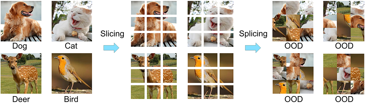
Splicing Operation: \[\begin{align} & \overline{x} = OP_{splice}([p_0^{x^0}, p_1^{x^1}, ..., p_{k*k-1}^{x^{k*k-1}}], k) \\ & st. \; \;( c(x^0)==c(x^1)==...==c(x^{k*k-1})) = False \end{align}\] where \(k\times k\) numbers of patches with uniform size that are sliced from images with different categories (denoted by \(c(\cdot)\)) are spliced into an image with the same size as \(x\) (see Fig. 2). Particularly, those patches are required to be not from images with the same categories.
Since the resulting seed examples do not belong to any categories visually (see Fig. 2), and thus are OOD examples. Note that, we just provide two simple operations for the splicing of image patches. More complex operations (e.g., considering angles, scales and rotation) could be extended easily, but is out of the scope of this paper.
4.2 Generating CODEs↩︎
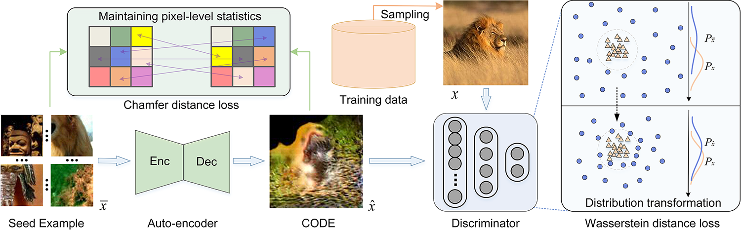
We transform the distribution of seed examples to that of the training data by feeding them into a novel Chamfer generative adversarial network (Chamfer GAN) with maintaining pixel-level statistics, to generate CODEs. In this following, we will describe the architecture design of Chamfer GAN first, and then discuss why CODEs generated by Chamfer GAN are effective OOD examples.
4.2.1 Chamfer GAN↩︎
For the design of Chamfer GAN, we adopt the popular auto-encoder [59] as our backbone, see Fig. 3. Given a seed example \(\bar{x}\) as input, the encoder \(Enc\) projects it into high-dimensional compact space, and the decoder \(Dec\) decode the projected feature to reconstruct the CODE \(\hat{x}\). Particularly, we adopt the Wasserstein distance loss in WGAN [60] to transform the data distribution, and the Chamfer distance loss [61] to maintain pixel-level statistics.
Wasserstein distance loss. To enforce the distribution of \(\hat{x}\) (i.e., \(P_{\hat{x}}\)) to be close to that of the training data \(x\) (i.e., \(P_{x}\)), we adopt the same adversarial loss as in WGAN [60] with the gradient penalty term omitted for clarity, which is defined as:
\[\label{eq:wgan} L_\text{WD} = {\mathbb{E}_{x \sim P_{x}}} [Dis(x)] - {\mathbb{E}_{\hat{x} \sim P_{\hat{x}}}} [Dis(\hat{x})]\tag{1}\]
\[\label{eq:general95cd} \begin{align} L_{\text{CD}} = {{\mathbb{E}}_{\bar{x}{\sim}P_{\bar{x}}}} & \bigg({ \sum_{\hat{x_i} \in \hat{{x}}} \min_{\bar{x_j} \in \bar{x}} \|\hat{x_i}-\bar{x_j}\|_2^{2}} \\ &+ \sum_{\bar{x_j} \in \bar{x}} \min_{\hat{x_i} \in \hat{{x}}} {\|\hat{x_i}-\bar{x_j}\|_2^2}\bigg) \\ &{st.} \; \hat{x} = Dec(Enc(\bar{x})) \end{align}\tag{2}\]
Chamfer distance loss. To facilitate maintaining pixel-level statistics during the reconstruction process, we adopt the Chamfer distance for restriction, which is defined as:
\[\label{zlfwquch} L_{\text{CD}} = {{\mathbb{E}}_{\bar{x}{\sim}P_{\bar{x}}}} \bigg({ \sum_{\hat{x_i} \in \hat{{x}}} \min_{\bar{x_j} \in \bar{x}} \|\hat{x_i}-\bar{x_j}\|_2^{2}} + \sum_{\bar{x_j} \in \bar{x}} \min_{\hat{x_i} \in \hat{{x}}} {\|\hat{x_i}-\bar{x_j}\|_2^2}\bigg)\tag{3}\]
\[\label{eq:general95cd95cons} \hat{x} = Dec(Enc(\bar{x}))\tag{4}\] where \(P_{\bar{x}}\) is the distribution that seed example \(\bar{x}\) is in, \(\bar{x_j}\) and \(\hat{x_i}\) denote the pixel in \(\bar{x}\) and \(\hat{x}\) respectively. Note that, we do not require \(\bar{x}\) and \(\hat{x}\) to be extremely the same which is enforced by \(L_2\) loss in traditional auto-encoder. Instead, the Chamfer distance loss enforces each pixel in \(\bar{x}\) to have a corresponding pixel in \(\hat{x}\) outputted by \(Enc\)-\(Dec\), but could at a different location, namely with pixels rearranged. Therefore, the pixel-level statistics is maintained.
By combining the above two loss functions, Chamfer GAN could transform the distribution of \({\hat{x}}\) to be close to that of the training data \(x\), while maintaining the pixel-level statistics of \(\bar{x}\). The final loss function is thus as follows: \[\label{eq:chamferGAN} L_{\bar{x}\rightarrow\hat{x}} = {\alpha}L_{\text{WD}} + L_{\text{CD}}\tag{5}\] where \(\alpha\) is a scalar weight set by \(1.0\mathrm{e}{-5}\) by default. For the training of Chamfer GAN, we train the classifier \(Dis\) and \(Enc\)-\(Dec\) in an iterative manner as in WGAN. Note that, the Chamfer distance loss is critical for Chamfer GAN. Specifically, Chamfer distance loss restricts the distribution transforms along a special feature space whose corresponding image space is a “pixel rearranged space”.
By feeding seed examples into Chamfer GAN, CODEs are obtained that maintain pixel-level statistics of seed examples, but within a distribution much closer to that of the training data.
4.2.2 Discussion on CODEs↩︎
Since with supervision by the Wasserstein distance loss, the distribution of CODEs is transformed to be close to that of the training data. Besides, CODEs remain to be OOD, due to: 1) the pixel-level statistics of seed examples that are originally OOD are maintained by the Chamfer distance loss; and 2) the training of WGAN that transforms the distribution to be the same as that of the training data is hard originally, and it is even harder with the restriction of Chamfer distance loss. Overall, CODEs are effective OOD examples. Please refer to Sec. 5.1 for validation.
4.3 Using CODEs against OOD Overconfidence↩︎
CODEs could be utilized to alleviate the OOD overconfidence issue by suppressing predictions on them over each category, namely enforcing averaged confidences over all categories (i.e., \(\frac{1}{K}\)) with the following loss function:
\[\label{adv95train} L_{sup}(\hat{x}) = \sum_{i=1}^{i=K} \frac{1}{K} \log{V_i(\hat{x})}\tag{6}\]
where \(K\) is the category number and \(V_i(\hat{x})\) is the normalized prediction confidence of \(\hat{x}\) over category \(i\).
For training, we adopt 50% images from the original training set supervised with the cross-entropy loss, while the others are CODEs supervised with Eqn. 6 .
5 Experiments↩︎
This section includes four parts. Firstly, we analyze the features of CODEs. Secondly, we extensively evaluate CODEs for alleviating the OOD overconfidence issue inherently with comparing with the state-of-the-art methods. Thirdly, we demonstrate the applications of CODEs, e.g., for improving OOD detection and classification. Finally, we report the ablation studies.

5.1 Features of CODEs↩︎
Implementation. We set \(k\) as 2 for generating seed examples. The auto-encoders in Chamfer GAN for 32\(\times\)32 and 28\(\times\)28 images adopt four convolution layers to project images to the resolution of 2\(\times\)2 with channel number of 512, while the decoder is symmetric to the encoder, except replacing the convolutions with transposed ones. For \(224\times224\) images, we adopt the architecture in [62]. We train the Chamfer GAN with a batch size of 32 for 1800 epochs on CIFAR-10 and CIFAR-100, 800 epochs on SVHN, MNIST, FMNIST and CINIC-10, and 50 epochs on ImageNet. The optimizer and learning rate are the same as in WGAN [60]. For more details, please refer to the supplementary.
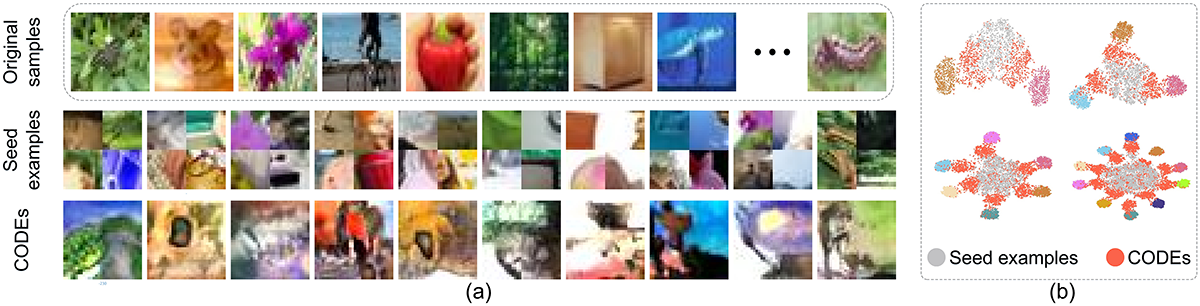
Visualization. Fig. 4 (a) visualizes seed examples, the corresponding CODEs, and original images from CIFAR-100. Fig. 4 visualizes the generated examples and the original images from CIFAR-100. The first row presents the seed examples, while the second row is the corresponding CODEs converted by Chamfer GAN. Visually, CODEs are more natural than seed examples, but we could not induce any categories on them, indicating that they are OOD examples. Fig. 4 (b) visualizes the t-SNE [63] embeddings of original images, seed examples and CODEs on CIFAR-10. Specifically, the embeddings are based on the features outputted by the last convolutional layer of ResNet-18. It demonstrates that the distributions of CODEs are much closer to that of clusters of original images compared with seed examples, validating the usefulness of Chamfer GAN for distribution transformation.
Distribution Distance and Prediction Confidence. We report the distribution distances between seed examples, CODEs and the original images in CIFAR-10, CIFAR-100 and SVHN, measured by Fréchet Inception Distance (FID) [64] in Tab. 1. It could be seen that the distribution distances between CODEs and original images are much smaller than that of seed examples, validating the process of distribution transformation. Particularly, with a closer distribution to that of the original images, CODEs are predicted by ResNet-18 with higher confidences.
| CIFAR-10 | CIFAR-100 | SVHN | ||
|---|---|---|---|---|
| FID | Seeds examples | 50.49 | 48.83 | 83.51 |
| CODEs | 36.53 | 36.53 | 77.94 | |
| MMC (%) | Origin | 98.40 | 91.28 | 99.42 |
| Seeds examples | 72.53 | 38.90 | 72.37 | |
| CODEs | 74.84 | 40.20 | 78.74 | |
5.2 Alleviating OOD Overconfidence by CODEs↩︎
| metric | test set | Baseline | CEDA | ACET | CCUs | Ours | Ours++ | OE | CCUd | |
|---|---|---|---|---|---|---|---|---|---|---|
| with auxiliary dataset | ✔ | ✔ | ||||||||
| TE | CIFAR-10 | 5.38 | 5.38 | 5.61 | 5.56 | 5.58 | 5.52 | 5.75 | 6.01 | |
| ID MMC | CIFAR-10 | 97.04 | 97.51 | 96.60 | 97.27 | 97.15 | 96.77 | 88.87 | 80.26 | |
| OOD MMC | SVHN | 73.38 | 72.46 | 70.69 | 74.13 | 62.37 | 47.18 | 10.48 | 10.41 | |
| CIFAR-100 | 79.47 | 80.54 | 79.28 | 80.83 | 70.14 | 59.52 | 21.62 | 16.98 | ||
| LSUN_CR | 73.38 | 75.15 | 75.89 | 75.95 | 64.11 | 53.67 | 10.56 | 10.38 | ||
| Noise | 69.24 | 10.36 | 10.62 | 77.85 | 10.27 | 10.89 | 13.37 | 10.36 | ||
| Uniform | 99.49 | 73.23 | 10.00 | 10.00 | 65.30 | 10.00 | 10.35 | 10.00 | ||
| Adv. Noise | 100.00 | 98.50 | 11.20 | 10.01 | 15.80 | 10.29 | 100.00 | 10.00 | ||
| Adv. Samples | 100.00 | 100.00 | 63.30 | - | 54.40 | 27.79 | - | - | ||
| TE | CIFAR-100 | 23.34 | 23.54 | 24.01 | 24.13 | 23.22 | 23.55 | 25.51 | 26.53 | |
| ID MMC | CIFAR-100 | 80.54 | 81.85 | 80.64 | 81.78 | 82.21 | 80.77 | 59.55 | 47.29 | |
| OOD MMC | SVHN | 61.15 | 57.91 | 39.54 | 51.02 | 44.34 | 32.50 | 3.96 | 2.26 | |
| CIFAR-10 | 52.13 | 55.23 | 54.30 | 55.58 | 52.82 | 49.10 | 15.56 | 8.49 | ||
| LSUN_CR | 53.19 | 51.41 | 54.22 | 52.34 | 51.33 | 48.01 | 3.10 | 1.60 | ||
| Noise | 61.40 | 57.89 | 19.27 | 57.67 | 19.96 | 14.92 | 10.94 | 7.84 | ||
| Uniform | 59.62 | 34.05 | 1.00 | 1.00 | 1.77 | 1.00 | 2.03 | 1.00 | ||
| Adv. Noise | 100.00 | 98.50 | 1.30 | 1.00 | 6.50 | 1.00 | 100.00 | 1.00 | ||
| Adv. Samples | 99.90 | 99.90 | 86.30 | - | 12.90 | 4.30 | - | - | ||
| TE | SVHN | 2.89 | 2.88 | 3.05 | 3.07 | 3.02 | 2.84 | 4.05 | 3.05 | |
| ID MMC | SVHN | 98.47 | 98.58 | 98.52 | 98.62 | 98.45 | 98.69 | 96.93 | 98.07 | |
| OOD MMC | CIFAR-10 | 71.94 | 71.70 | 69.28 | 68.40 | 61.09 | 50.78 | 10.14 | 10.14 | |
| CIFAR-100 | 71.76 | 71.04 | 68.78 | 68.63 | 54.09 | 53.46 | 10.16 | 10.20 | ||
| LSUN_CR | 71.27 | 71.06 | 62.18 | 65.78 | 36.45 | 29.98 | 10.14 | 10.09 | ||
| Noise | 72.00 | 68.87 | 39.89 | 63.43 | 35.58 | 33.53 | 35.57 | 48.81 | ||
| Uniform | 67.80 | 40.06 | 10.00 | 10.00 | 10.34 | 10.00 | 10.10 | 10.00 | ||
| Adv. Noise | 100.00 | 94.60 | 10.10 | 10.00 | 24.30 | 11.00 | 100.00 | 10.00 | ||
| Adv. Samples | 100.00 | 99.50 | 36.90 | - | 38.70 | 11.40 | - | - | ||
| TE | MNIST | 0.51 | 0.50 | 0.50 | 0.49 | 0.47 | 0.51 | 0.75 | 0.51 | |
| ID MMC | MNIST | 99.18 | 99.16 | 99.15 | 99.16 | 98.99 | 99.34 | 99.27 | 99.16 | |
| OOD MMC | FMNIST | 66.31 | 52.88 | 28.58 | 63.93 | 35.32 | 20.98 | 34.38 | 25.99 | |
| EMNIST | 81.95 | 81.81 | 77.92 | 83.01 | 69.54 | 47.78 | 88.00 | 77.74 | ||
| GrCIFAR-10 | 46.41 | 19.10 | 10.10 | 10.02 | 10.43 | 10.00 | 11.50 | 10.00 | ||
| Noise | 12.70 | 12.09 | 10.36 | 10.59 | 10.51 | 10.00 | 10.22 | 10.34 | ||
| Uniform | 97.33 | 10.01 | 10.00 | 10.00 | 10.01 | 10.40 | 10.01 | 10.00 | ||
| Adv. Noise | 100.00 | 14.70 | 16.20 | 10.00 | 12.50 | 10.00 | 100.00 | 10.00 | ||
| Adv. Samples | 99.90 | 98.20 | 85.40 | - | 63.80 | 45.20 | - | - | ||
| TE | FMNIST | 4.77 | 5.01 | 4.78 | 4.85 | 4.56 | 4.79 | 6.12 | 4.96 | |
| ID MMC | FMNIST | 98.38 | 98.24 | 98.03 | 98.32 | 98.44 | 98.35 | 98.30 | 98.46 | |
| OOD MMC | MNIST | 71.32 | 73.44 | 73.70 | 71.25 | 69.67 | 61.47 | 80.34 | 70.54 | |
| EMNIST | 65.01 | 67.34 | 66.63 | 68.68 | 62.97 | 59.13 | 36.66 | 31.62 | ||
| GrCIFAR-10 | 86.17 | 69.69 | 72.90 | 56.33 | 66.88 | 63.24 | 10.22 | 10.09 | ||
| Noise | 67.72 | 57.40 | 16.75 | 56.84 | 14.71 | 13.03 | 10.45 | 10.25 | ||
| Uniform | 77.70 | 60.08 | 10.00 | 20.00 | 10.00 | 10.06 | 73.16 | 10.00 | ||
| Adv. Noise | 100.00 | 22.30 | 16.78 | 10.00 | 14.99 | 10.18 | 100.00 | 10.00 | ||
| Adv. Samples | 100.00 | 99.67 | 90.56 | - | 70.14 | 59.43 | - | - | ||
Datasets. Various datasets are used: CIFAR-10, CIFAR-100 [65], GrCIFAR-10 (gray scale CIFAR-10), SVHN [66], LSUN_CR (the classroom subset of LSUN [67]), MNIST, FMNIST [68], EMNIST [69], Noise (i.e., randomly permuting pixels of images from the training set as in [21]), Uniform (i.e., uniform noise over the \([0, 1]^d\) box as in [21]), Adversarial Noise and Adversarial Sample following the experimental setting as [21]. Adversarial Noise is generated by actively searching for images which yield higher prediction confidences in a neighbourhood of noise images, while Adversarial Sample is generated in a neighbourhood of in-distribution images but are off the data manifold following [11]. For OE and CCUd, we adopt 80 Million Tiny Images [70] with all examples that appear in CIFAR-10 and CIFAR-100 removed as the auxiliary dataset as in [21].
Methods. Eight methods are evaluated and compared: Baseline, CEDA [11], ACET [11], OE [9], two variants of CCU [21] (CCUs that adopts noise and CCUd that adopts an auxiliary dataset as in [9]), Ours and Ours++. Particularly, Ours++ is an enhanced version of Ours, with selecting the worst cases, i.e., have the largest prediction confidences, in a neighborhood of CODEs similar as in ACET [11].
. We train LeNet on MNIST and FMNIST while ResNet-18 for CIFAR-10, CIFAR-100 and SVHN, and then evaluate them on the corresponding test set to report the test error (TE), and on both in- and out-of-distribution datasets to report mean maximal confidence (MMC) following [21].
Comparisons with the State-of-the-art Methods. The results in Tab. 2 show that Ours and Ours++ perform the best in most cases without considering OE and CCUd on CIFAR-10, CIFAR-100 and SVHN. Since training with suppressing the predictions on the large 80 Million Tiny Images [70], that has similar image style as the OOD datasets (e.g., CIFAR-10, CIFAR-100 and SVHN), OE and CCUd obtain the lowest MMCs. However, it could be seen that the auxiliary dataset brings a detrimental impact on the predictions on in-distribution samples, e.g., 33% lower prediction confidences on CIFAR-100 for CCUd, and thus leads to worse classification performance, e.g., 3.2% larger test error. Besides, for datasets that have large differences with the auxiliary dataset, OE and CCUd are comparable with and even worse than Ours and Ours++, e.g., on FMNIST and MNIST.
Particularly, ACET performs better than CEDA, validating the usefulness of the strategy that searches harder examples in a neighbourhood of the original ones. We would like to point out that our method is comparable with ACET even without picking harder examples, indicating that CODEs are more effective than random noises. By applying the same strategy to Ours, we could see significant drops in MMC values. For Adversarial Noise and Adversarial Sample, we could see that CEDA and OE fail in most cases, ACET could handle part of samples, while Ours++, CCUs and CCUd perform the best. Overall, CODEs are effective in alleviating the OOD overconfidence issue.
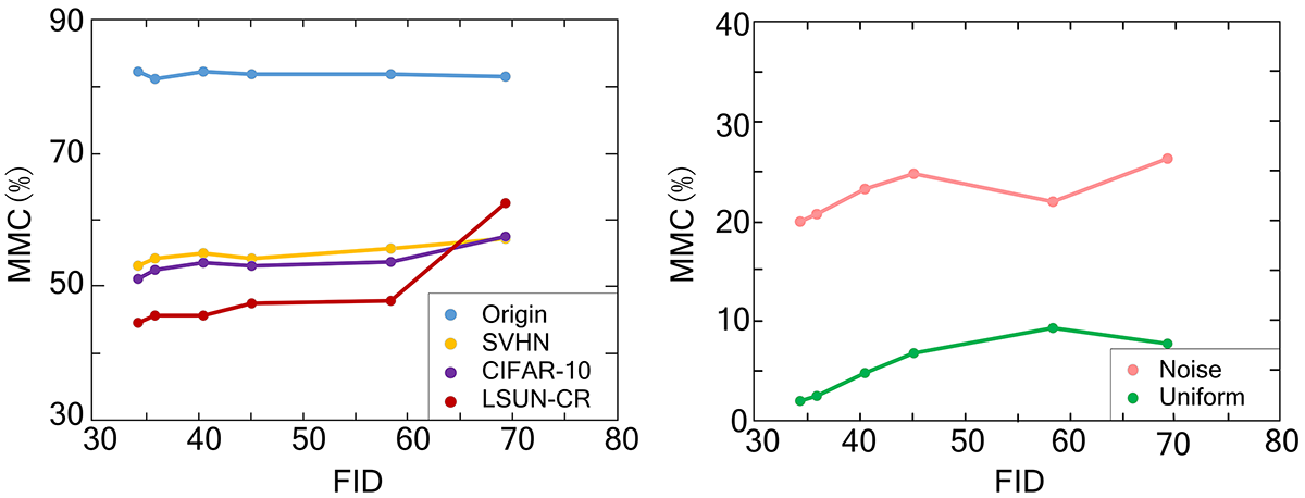
Distribution Distance vs. MMC. We investigate how distribution distance between CODEs and the in-distribution data would affect the benefits brought by suppressing CODEs on alleviating the OOD overconfidence issue. Since we apply a relatively high weight \(1.0\) to the Chamfer distance loss, while a low weight \(1.0\mathrm{e}{-5}\) to Wasserstein distance loss, the distribution transforming could be carried on gradually during the training process. To facilitate fair comparisons, we choose the models of Chamfer GAN saved at different epochs during the training stage on CIFAR-100, including models of 200\(th\), 400\(th\), 800\(th\), 1200\(th\), 1600\(th\) and 1800\(th\), and then train ResNet-18 models with suppressing predictions on the CODEs outputted by the above six Chamfer GANs respectively. Fig. 6 shows that MMCs are mostly positively relevant to the FID scores, and the correlation is stronger on OOD datasets than on Noise and Uniform, validating that smaller distribution distance to the in-distribution samples is critical for effective OOD examples. We also report the MMCs on in-distribution samples of the six different ResNet-18 models in Fig. 6, and could see the MMCs mostly remain unchanged.
Indeed, OE have also mentioned the influence of distribution distance [9]. However, since the difference between different auxiliary datasets could have many different factors, e.g., RGB values, local textures, it is thus not suitable to conclude which factor affects the result. Differently, we transform the distribution of seed examples with Chamfer distance loss to maintain the low-level pixel statistics, such that could rule out the influence of many other factors.
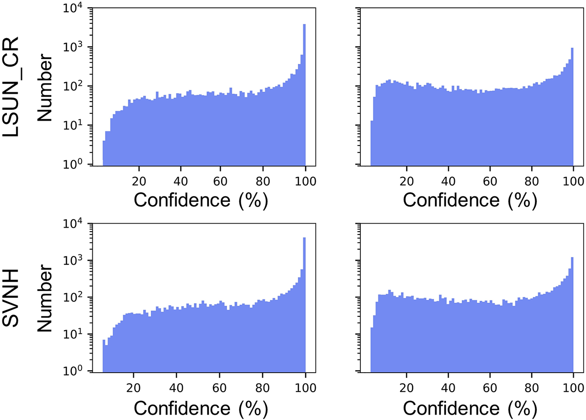
Visualization of Maximum Confidence. We visualize the maximum confidences predicted on the images in LSUN_CR and SVHN by ResNet-18 trained on CIFAR-100 using logarithmic histograms in Fig. 7. It could be seen that, by adopting our method, the confidence distributions made by Baseline are pulled to the left, with the number of samples with high confidence largely reduced.
In-distribution Confidence Calibration. We report expected calibration errors (ECEs) [36] of ResNet-18 trained on CIFAR-10/100 and test on the corresponding test set in Tab. 3. It could be seen that ECEs are reduced after applying our method, while temperature tuning is more effective in calibrating prediction confidence on in-distribution data.
| CIFAR-10 | CIFAR-100 | |||
| Before TT | After TT | Before TT | After TT | |
| w/o Ours | 0.033 | 0.031 | 0.081 | 0.073 |
| w/ Ours | 0.008 | 0.006 | 0.059 | 0.042 |
5.3 Applications of CODEs↩︎
5.3.1 Improving OOD Detection↩︎
Evaluation Strategy and Metrics. We follow the evaluation strategy as in [5] and use the three common metrics: the false positive rate of OOD examples when true positive rate of in-distribution examples is at 95% (FPR95), the area under the receiver operating characteristic curve (AUROC), and the area under the precision-recall curve (AUPR).
| FPR95 \(\downarrow\) | AUROC \(\uparrow\) | AUPR \(\uparrow\) | ||
|---|---|---|---|---|
| CIFAR-10 | OE | 8.53 | 98.30 | 99.63 |
| OE+ | 8.01 | 99.07 | 99.79 | |
| ES | 3.32 | 98.92 | 99.75 | |
| ES+ | 3.24 | 99.01 | 99.78 | |
| CIFAR-100 | OE | 58.10 | 85.19 | 96.40 |
| OE+ | 56.54 | 87.96 | 97.38 | |
| ES | 47.55 | 88.46 | 97.12 | |
| ES+ | 45.89 | 89.03 | 97.95 | |
Methodology. We replace the original DNN classifier with the one trained with suppressing predictions on CODEs.
Improving OOD detectors. We first evaluate the improvement on OE [9] and Energy Score [24] that use 80 Million Tiny Images [70] as the auxiliary dataset. Specifically, we train WRN-40-2 [71] on CIFAR-10 and CIFAR-100 [65], and then test it on six datasets: Textures [72], SVHN, Places365 [73], LSUN-Crop [67], LSUN-Resize [67], and iSUN [74] following [24]. The averaged results in Tab. 4 show that the performance on all three metrics are improved. We also evaluate the improvement on ODIN [6] and Mahalanobis distance (Maha) [23] that do not require auxiliary datasets. The results in Tab. 5 show that both ODIN and Maha are improved. Overall, CODEs could be adopted for improving OOD detectors.
| ODIN | ODIN+ | Maha | Maha+ | ||
|---|---|---|---|---|---|
| CIFAR-10 | 95.91 | 96.90 | 97.10 | 97.34 | |
| CIFAR-100 | 94.82 | 97.12 | 96.70 | 97.08 | |
| LSUN_CR | 96.52 | 96.96 | 97.22 | 97.97 | |
| Noise | 82.74 | 83.01 | 98.00 | 97.99 | |
| Uniform | 97.90 | 97.94 | 97.81 | 98.01 | |
| SVHN | 81.35 | 84.91 | 77.52 | 79.63 | |
| CIFAR-10 | 79.50 | 83.48 | 59.94 | 64.74 | |
| LSUN_CR | 81.41 | 82.10 | 79.73 | 82.99 | |
| Noise | 76.84 | 76.92 | 90.61 | 90.98 | |
| Uniform | 93.56 | 94.87 | 94.37 | 95.90 | |
![Figure 8: PR curves of four methods for the semantic OOD detection task [75] on CIFAR-10 with holding out one class as OOD.](/article/2108.06024/images/PRCurve3.png "fig:")
| Baseline | Baseline+ | ||
|---|---|---|---|
| CINIC-10 | ResNet-32 | 73.82 | 74.77 |
| ResNet-56 | 74.09 | 75.38 | |
| ImageNet | ResNet-18 | 69.76 | 71.06 |
| ResNet-50 | 76.15 | 77.12 | |
Detecting Semantic OOD Examples. We evaluate the situation where in-distribution samples are not only significantly outnumber OOD ones, but also have significant semantic shifts following [75]. Specifically, we train two classifiers for CIFAR-10 with holding out one class every time (e.g., plane, cat), and then score the ability to detect the held out class as OOD samples. The precision-recall curves are presented in Fig. 8. It could be seen that OE [9] and CCUd [21] that adopt auxiliary datasets hurt the performance of semantic OOD detection since predictions on in-distribution samples are suppressed as reported in Tab. 2, while utilizing CODEs is beneficial to it.
5.3.2 Improving Classification↩︎
We demonstrate CODEs could improve classification by evaluating ResNets on CINIC-10 [76] and ImageNet [77]. Particularly, a separate batch norm for CODEs is adopted following [41], which is critical for consistent improvement. The results in Tab. 6 show that CODEs bring 1-2 percent improvement on the top-1 accuracy. The reason is probably that CODEs are sampled in between the decision boundaries of multiple categories since are spliced with patches from different-category images, and thus could help to prevent confusion between multiple different categories.
| CIFAR-100 | CIFAR-10 | SVHN | |
|---|---|---|---|
| Baseline | 78.99 | 57.50 | 70.95 |
| w/o Chamfer GAN | 50.23 | 58.08 | 59.67 |
| w/ Chamfer GAN | 43.64 | 54.44 | 51.62 |
| 2 | 4 | 6 | 8 | |
|---|---|---|---|---|
| MMC | 43.64 | 47.89 | 46.32 | 48.39 |
5.4 Ablation Studies↩︎
Setup. We train different ResNet-18 models with suppressing predictions on CODEs generated with/without Chamfer GAN, and with different \(k\)s in the slicing&splicing operations, and then test them on OOD datasets listed in Tab. 2 to report averaged MMC results in Tab. 7 and Tab. 8.
Chamfer GAN. It could be seen that ResNet-18 models trained with ablating Chamfer GAN still improve the performance, since the distribution of seed examples are originally close to the ID distribution with the novel slicing&splicing operation as reported in Tab. 2. However, the performance is much worse than that with Chamfer GAN, validating the importance of distribution transformation.
Piece \(k\). It could be seen that \(k=2\) brings the best performance in Tab. 8, since larger \(k\) may bring too more flexibility for Chamfer GAN to maintain the pixel-level statistics.
Chamfer GAN. We compare MMCs predicted by ResNet-18 trained with suppressing CODEs generated with and without Chamfer GAN on five OOD datasets listed in Tab. 2 except Adversarial Noise and Adversarial Sample. The averaged results in Tab. 7 show that ablating Chamfer GAN hurts the performance, validating its importance. We summarize the averaged MMCs predicted by ResNet-18 trained with suppressing CODEs generated with and without Chamfer GAN on five OOD datasets listed in Tab. 2 except Adversarial Noise and Adversarial Sample. The results in Tab. 7 show that ablating Chamfer GAN hurts the performance, validating its importance. Piece \(k\). We summarize the averaged MMCs predicted by ResNet-18 trained with suppressing CODEs generated with different \(k\)s in the slicing&splicing operations in Tab. 8. It could be seen that \(k=2\) brings the best performance.
6 Conclusion↩︎
This paper has proposed CODEs, a kind of effective OOD examples that could be utilized to alleviate the OOD overconfidence issue inherently by suppressing predictions on them. The key idea of generating CODEs is to restrict the distribution of spliced OOD examples generated from training data, to be close to that of in-distribution samples by Chamfer GAN. Extensive experiments validate the effectiveness of CODEs and their usefulness in improving OOD detection and classification. We hope CODEs inspire more research on alleviating the OOD overconfidence issue.
This work was supported in part by the Guangdong Basic and Applied Basic Research Foundation (2020A1515110997), the NSFC (U20B2046, 61902082, 62072126), the Science and Technology Program of Guangzhou (202002030263, 202102010419), the Guangdong Higher Education Innovation Group (2020KCXTD007) and the Talent Cultivation Project of Guangzhou University (XJ2021001901).
This paper has proposed Chamfer OOD examples (CODEs), a kind of effective OOD examples that could alleviate the OOD overconfidence issue by suppressing predictions on them. They are generated by applying slicing&splicing operations and feeding into Chamfer GAN, with training data only. Extensive experiments validate the effectiveness of CODEs and show our method would not bring any detrimental impact on in-distribution samples. We also demonstrate CODEs are beneficial to improve OOD detection and classification. We hope CODEs inspire more researches against the OOD overconfidence issue.
whose distribution is close to that of in-distribution samples are effective for satisfying three core properties of effective OOD examples is critical to enable OOD examples to take effect in adversarial training. To fulfill the three properties, we propose slicing&splicing operations and Chamfer GAN. Extensive experiments validate the effectiveness of CODEs. We hope our definition of effective OOD examples could inspire more researches on OOD overconfidence issue and OOD examples.
This paper has proposed Chamfer OOD examples (CODEs) to alleviate the overconfidence issue on out-of-distribution (OOD) samples.
The effectiveness of CODEs is derived from three core properties: negative, adversarial to positive and distribution-restricted. To approach that, we propose Charmfer GAN as well as constraints, to generate CAEs t the properties.
which is a kind of effective OOD examples (OOD examples)
The key of is to satisfy three core properties of effective OOD examples.
idea is that satisfying three core properties of effective OOD examples is critical to enable OOD examples to take effect in adversarial training.
we adopt slicing&splicing operations and a novel Chamfer GAN to enforce CODEs to be effective.
To fulfill the three properties, we adopt slicing&splicing operations and a novel Chamfer GAN to enforce CODEs to be effective. Extensive experiments validate the effectiveness of CODEs. We hope our definition of effective OOD examples could inspire more research on OOD overconfidence issue and OOD examples.
This paper, we aim to devise a OOD examples (OOD examples) to alleviating the out-of-distribution overconfidence.