Secure Quantized Training for Deep Learning
July 01, 2021
Abstract
We implement training of neural networks in secure multi-party computation (MPC) using quantization commonly used in said setting. We are the first to present an MNIST classifier purely trained in MPC that comes within 0.2 percent of the accuracy of the same convolutional neural network trained via plaintext computation. More concretely, we have trained a network with two convolutional and two dense layers to 99.2% accuracy in 3.5 hours (under one hour for 99% accuracy). We have also implemented AlexNet for CIFAR-10, which converges in a few hours. We develop novel protocols for exponentiation and inverse square root. Finally, we present experiments in a range of MPC security models for up to ten parties, both with honest and dishonest majority as well as semi-honest and malicious security.
1 Introduction↩︎
Secure multi-party computation (MPC) is a cryptographic technique that allows a set of parties to compute a public output on private inputs without revealing the inputs or any intermediate results. This makes it a potential solution to federated learning where the sample data stays private and only the model or even only inference results are revealed.
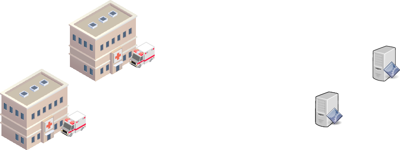
Imagine a set of healthcare providers holding sensitive patient data. MPC allows them to collaboratively train a model. This model could then either be released or even kept private for inference using MPC again. See Figure 1 for an illustration. Note that MPC is oblivious to how the input data is split among participants, that is, it can be used for the horizontal as well as the vertical case.
A more conceptual example is the well-known millionaires’ problem where two people want to find out who is richer without revealing their wealth. There is clearly a difference between the one bit of information desired and the full figures.
There has been a sustained interest in applying secure computation to machine learning and neural networks going back to at least [1]. More recent advances in practical MPC have led to an increased effort in implementing both inference and training.
A number of works such as [2], [3], [4], [5] implement neural network training with MPC at least in parts. However, for the task of classifying MNIST digits, they either give accuracy figures below 95% or figures obtained using plaintext training. For the latter case, the works do not clarify how close the computation for plaintext training matches the lower precision and other differences in the MPC setting. [6] achieved an accuracy of 99.38% in a comparable setting for a convolutional neural network with more channels than we use. However, their actual implementation only uses dense layers, and we achieve comparable accuracy in this model. All works use quantization in the sense that a fractional number \(x\) is represented as \(\lfloor x \cdot 2^{f} \rceil\) where \(\lfloor \cdot \rceil\) denotes rounding to the nearest integer, and \(f\in\mathbb{Z}\) (\(\mathbb{Z}\): the set of integers) is a precision parameter. This makes addition considerably faster in the secure computation setting because it reduces to integer addition (at the cost of compounding rounding errors). Furthermore, some of the works suggest replacing the softmax function that uses exponentiation with a ReLU-based replacement. [7] discovered that this softmax replacement deteriorates accuracy in multilayer perceptrons to the extent that it does not justify the efficiency gains.
The concurrent work of [8] gives some figures on the learning curves when trained with secure computation. However, they stop at five epochs for MNIST training and achieve 94% accuracy, whereas we present the figures up to 50 epochs and 99.2% accuracy using AMSGrad. Our implementation using stochastic gradient descent (SGD) is 40% faster than theirs. Note that we use the CPU of one AWS c5.9xlarge instance per party whereas [8] use one NVIDIA Tesla V100 GPU per party. We believe this somewhat counter-intuitive result comes from MPC heavily relying on communication, which is an aspect where GPUs do not have an advantage over CPUs. While GPUs are very efficient in computing on data in their cache, it is no more efficient to transfer data in and out of these caches.
In this paper, we present an extensible framework for secure deep learning based on MP-SPDZ by [9], a software library for multi-party computation.1 Similar to TensorFlow and PyTorch, our approach allows representing deep learning models as a succession of layers. We then use this implementation to obtain accuracy figures for MNIST and CIFAR-10 training by utilizing the MP-SPDZ emulator, which allows to run the plaintext equivalent of secure computation, that is, the same algorithms with the same precision. Finally, we run one of the most promising instantiations in real secure computation in order to benchmark it, confirming the results from the plaintext emulator. We use less sophisticated datasets because the relatively high cost of MPC makes is less feasible to use datasets with millions of examples rather than tens of thousands.
For our implementation, we have designed novel protocols for exponentiation and inverse square root computation. Both play an important role in deep learning, the first in softmax, and the second in the Adam and AMSGrad optimizers. Our protocols are based on mixed-circuit computation, that is, we combine a protocol that works over \(\mathbb{Z}_M\) for some large modulus \(M\) and thus integer-like computation with a protocol in the same security model that works over \(\mathbb{Z}_2\), which allows computing binary circuits.2
There are several projects that integrate secure computation directly into popular machine learning frameworks such as CrypTen by [10], PySyft by [11], and TF Encrypted by [12]. Our approach differs
from all of them by running the protocol as native CPU code (implemented using C++). This allows for much faster execution. For example, CrypTen provides an MNIST training example (mpc_autograd_cnn), which we adapted to full
LeNet [13] training. It took over three hours to run one epoch on one machine. In comparison, our implementation takes 11 minutes to run
one epoch with the full dataset of 60,000 samples with the same hardware across instances.
An alternative to MPC would be using purely homomorphic encryption. [14] trained an MNIST network to 98.6% accuracy in 8 days whereas we achieved the same accuracy in less than 5 days when using a two-party protocol based on homomorphic encryption.
A number of works [15]–[17] only implemented deep learning inference. None of them implements all building blocks necessary for training. It is therefore not possible to make any statement on the training performance of these works.
Another line of work (e.g., [18]) uses trusted execution environments that provide computation outside the reach of the operating system. This is a different security model to multi-party computation that works with distributing the information among several entities.
The rest of this paper is structured as follows: We highlight some secure computation aspects in Section 2 and do the same for machine learning in Section 3. Section 4 analyzes the error introduced by the quantization. Finally, we present our implementation and our experimental results for MNIST and CIFAR-10 classification in Section 5.
2 Secure Computation Building Blocks↩︎
Our secure implementation has two layers of abstraction. The lower level is concerned with a few basic operations that depend on the actual protocol and security model. The basic operations include integer addition and multiplication, input, output, and domain conversion, that is converting between integer-focused and bit-focused computation. Appendices 7 and 8 give the details of our honest-majority three-party protocol and our dishonest-majority protocol, respectively. Honest and dishonest majority refer to how many computing parties are being trusted. For an honest majority, strictly more than half parties must follow the protocol and not reveal information to anyone else. This setting allows for more efficient protocols while the dishonest-majority setting requires more expensive cryptographic schemes such as homomorphic encryption to be used. See [9] for a cost comparison between a range of protocols. The higher level of abstraction is common to all protocol as it builds in a generic way on the primitives in the lower level. Notable operations on this level are division, exponentiation, and inverse square root. Appendix 9 provides more details.
In this section, we focus on two aspects: How to implement fractional-number computation with integers, and how to implement exponentiation. The former plays a crucial role in efficient secure computation, and the latter presents a novel protocol. We also contribute a novel protocol for inverse square root computation, which is deferred to Appendix 9 due to space constraints.
2.1 Quantization↩︎
While [19] showed that it is possible to implement floating-point computation, the cost is far higher than integer computation. It is therefore common to represent fractional numbers using quantization (also called fixed-point representation) as suggested by [20]. A real number \(x\) is represented as \(Q^f(x)\mathrel{\mathop{:}}=\lfloor x \cdot 2^{f} \rceil\) where \(f\) is a positive integer specifying the precision. The linearity of the representation allows to compute addition by simply adding the representing integers. Multiplication however requires adjusting the result because it will have twice the precision: \((x \cdot 2^f) \cdot (y \cdot 2^f) = xy \cdot 2^{2f}\). There are two ways to rectify this:
An obvious correction would be to shift the result by \(f\) bits after adding \(2^{f-1}\) to the integer representation, as \(\lfloor xy\cdot{}2^{f} \rceil=\lfloor 2^{-f}\cdot (xy\cdot 2^{2f} + 2^{f-1}) \rfloor\), where \(\lfloor \cdot \rfloor\) is the floor function. This ensures rounding to the nearest number possible in the representation, with the tie being broken by rounding up.
However, [20] found that in the context of secure computation it is more efficient to use probabilistic truncation. This method rounds up or down probabilistically depending on the input. For example, probabilistically rounding 0.75 to an integer would see it rounded up with probability 0.75 and down with probability 0.25.
Our quantization scheme is related to quantized neural networks (see e.g. [21]). However, our consideration is not to compress the model, but to improve the computational speed and to reduce communication.
2.2 Exponentiation↩︎
![Figure 2: Exponentiation with base two [22]](/article/2107.00501/_pdflatex/bwcdexsm.png "fig:")
![Figure 3: Procedures in Algorithms 2 and [alg:our-exp]](/article/2107.00501/_pdflatex/vdmyikrj.png "fig:")
Exponentiation is a core computational module in deep learning and is useful to evaluate non-linear activation functions such as the softmax. [2] introduced a simplification of softmax to avoid computing exponentiation. In this section, we present an optimized exponentiation protocol instead.
As noted by [22], exponentiation can by reduced to exponentiation with base two using \(a^x = 2^{x \log_2 a}\). Furthermore, if the base is public, this reduction only costs one public-private multiplication, and it introduces an acceptable error as \[2^{x \log_2 a \pm 2^{-f}} = 2^{x \log_2 a} \cdot 2^{\pm 2^{-f}}.\] The second multiplicand on the right-hand side is easily seen to be within \([1 - 2^{-f}, 1 + 2^{-f}]\).
Algorithm 2 shows the exponentiation method by [22]. It uses \(\langle \cdot \rangle^{\mathsf{A}}\) to indicate integer sharing and \(\langle \cdot; f \rangle^{\mathsf{A}}\) to indicate fixed-point sharing. We use the superscript \(\mathsf{A}\) to indicate that both secret sharing are in the arithmetic domain, that is, in \(Z_M\) for some large \(M\). This distinguishes them from the bit-wise secret sharing indicated by \(\mathsf{B}\) used below. The algorithm uses a number of standard components such as addition, multiplication, comparison, and bit decomposition. Furthermore, it uses a polynomial approximation of \(2^x\) for \(x \in [0,1]\). They propose to use the polynomial \(P_{1045}\) by [23]. However, we found that Taylor approximation at 0 leads to better results than \(P_{1045}\).
Algorithm 2 suffers from two shortcomings. First, it is unnecessarily restrictive on negative inputs because it uses the absolute value of the input, the exponentiation of which falls outside the representation range for values as small as \(k - f - 1\) where \(k\) is a parameter defining the range of inputs (\([-2^{k-f-1},2^{k-f-1}]\)). Second, the truncation used to find the integer component resembles bit decomposition in many protocols. It is therefore wasteful to separate the truncation and the bit decomposition. Algorithm [alg:our-exp] fixes these two issues. It also explicitly uses mixed circuits, with binary secrets denoted using \(\langle \cdot \rangle^{\mathsf{B}}\).
The general structure of Algorithm [alg:our-exp] is the same as Algorithm 2. It splits the input into an integer and a fractional part and then computes the exponential separately, using an exact algorithm for the integer part and an approximation for the fractional part. It differs in that it uses mixed circuits and it allows any negative input. The biggest difference however is in step [step:trunc], where the exponentiation of a negative number is not computed by inverting the exponentiation of the absolute value. Instead, we use the following observation. If \(-2^\ell \le x < 0\), \(x = -2^\ell + y + r\), where \(y = x + 2^\ell - r\) and \(r\) is the fractional component of \(x\). Then, \[2^x = 2^{-2^\ell} \cdot 2^y \cdot 2^r.\] \(2^y\) equals \(d\) in Algorithm [alg:our-exp] because \(y\) is the composition of the bits used in integer exponentiation, namely \(y = \sum_{i=0}^{\ell-1} x_{f+i}\). Therefore, \(g \approx 2^y \cdot 2^r\), and \[g' \approx \frac{g}{2^{2^\ell}} \approx 2^x\] for \(g\) and \(g'\) in steps [step:g] and [step:gprime] because rounding by \(2^\ell\) bits implies division by \(2^{2^\ell}\). This saves a relatively expensive division compared to Algorithm 2.
Table 1 shows how the two algorithms compare in terms of communication across a number of security models. All figures are obtained using MP-SPDZ [9] with \(f=16\), \(k=31\), computation modulo \(2^{64}\) for three-party computation, and computation modulo a 128-bit prime for two-party computation (as in Section 5.1.1.1). We use edaBits for mixed-circuit computation in Algorithm [alg:our-exp]. Across all security models, our algorithm saves about 30 percent in communication despite the improved input range. In the context of the figures in Table [tbl:table:sec-models] the improvement is less than one percent because exponentiation is only used once for every example per epoch, namely for the computation of softmax.
| 3 Parties | 2 Parties | |||
| SH | Mal. | SH | Mal. | |
| [22] | 27 | 498 | 1,338 | 214,476 |
| Algorithm [alg:our-exp] (ours) | 16 | 323 | 813 | 121,747 |
3 Deep Learning Building Blocks↩︎
| Operation | MPC Cost (\(\approx\)) | Efficiency | |
|---|---|---|---|
| \(\iverson{x>y}\) | \(10^1\) | ||
| \(x\pm{y}\) | \(10^{-1}\) | ||
| \(x\times{y}\) (integer) | \(10^0\) | ||
| \(x\times{y}\) (fractional) | \(10^1\) | ||
| \(x/y\) | \(10^2\) | ||
| \(1/\sqrt{x}\) | \(10^2\) | ||
| \(\exp(x), \log(x)\) | \(10^2\) |
In this section, we give a high-level overview of our secure deep learning framework, and how it builds upon our low-level computational modules (implemented from scratch) to tackle challenges in secure computation. Table 2 shows a non-exhaustive list of basic operations that is our computational alphabet, with a rough estimation of their cost in MPC. The “MPC Cost” column shows how an operation relates to integer multiplication in terms of magnitude order because integer multiplication is the most basic operation that involves communication. Most notably, comparison is not the basic operation as in silicon computation.
3.0.0.1 Linear Operations
Matrix multiplication is the workhorse of deep learning frameworks. The forward and backward computation for both dense layers and convolutional layers are implemented as matrix multiplication, which in turn is based on dot products. A particular challenge in secure computation is to compute a number of outputs in parallel to save communication rounds. We overcome this challenge by having a dedicated infrastructure that computes all dot products for a matrix multiplication in a single batch of communication, thus reducing the number of communication rounds. Another challenge is the accumulated error when evaluating matrix multiplication using quantized numbers. The following Section 4 presents a careful analysis on our solution to this potential issue. Our secure computation implementation uses efficient dot products when available (Appendix 7) or efficient use of SIMD-style homomorphic encryption (Appendix 8).
3.0.0.2 Non-linear Operations
A major part of the non-linear computation is the non-linear neural network layers. Both rectified linear unit (ReLU; [24]) and max pooling are based on
comparison followed by oblivious selection. For example, \(\mathsf{ReLU}(x) \mathrel{\mathop{:}}=\max(x,0) = ( x>0~?~x~:~0 )\), where the C expression \((\mathrm{condition}~?~a~:~b)\) outputs \(a\) if \(\mathrm{condition}\) is true and outputs \(b\) if otherwise. In secure
computation, it saves communication rounds if the process uses a balanced tree rather than iterating over all input values of one maximum computation. For example, two-dimensional max pooling over a 2x2 window requires computing the maximum of four values.
We compute the maximum of two pairs of values followed by the maximum of the two results. Our softmax and sigmoid activation functions are implemented using the exponentiation algorithm in section 2.2. Another source of
non-linear computation is the inverse square root \(1/\sqrt{x}\), which appears in batch normalization [25], our secure
version of Adam [26] and AMSGrad [27] optimizers, and Glorot
initialization [28] of the neural network weights. Our novel implementation of \(1/\sqrt{x}\) (explained in Appendix 9.0.0.4) is more efficient than state-of-the-art alternatives [22], [29]. It helps to avoid numerical division, which is much more expensive than multiplication. Taking Adam as an example, the increment of the parameter \(\theta_i\) in each learning step is altered to \(\gamma g_i / \sqrt{v_i + \varepsilon}\) (\(\gamma\): learning rate; \(g_i\) and
\(v_i\): first and second moments of the gradient; \(\varepsilon=10^{-8}\)) as compared to \(\gamma g_i/\left(\sqrt{v_i} + \varepsilon\right)\) in [26]’s original algorithm, so that we only need to take the inverse square root of \(v_i + \varepsilon\), then multiply by \(\gamma\) and \(g_i\).
3.0.0.3 Random Operations
Our secure framework supports random initialization of the network weights [28], random rounding, random shuffling of the training samples, and Dropout [30]. Our implementation relies on uniform random samplers [31], [32] based on mixed-circuit computation. Random rounding and Dropout require to draw samples from Bernoulli random variables. By a reparameterization trick, a sample \(x\) from the distribution \(\mathrm{Prob}(x=a)=p\), \(\mathrm{Prob}(x=b)=1-p\) (\(\mathrm{Prob}(\cdot)\): probability of statement being true) can be expressed as \(x=b+(a-b)\lfloor p+r \rfloor\), where \(r\sim\mathcal{U}(0,1)\) (uniform distribution on \([0,1]\)).
4 An Analysis of Probabilistic Rounding↩︎
In this section, we analyze the rounding error of our secure quantized representation for matrix multiplication. We show that our rounding algorithm is unbiased; has acceptable error; is potentially helpful to training. Fixed point numbers [33] and stochastic rounding [34] have been applied to deep learning. The rounding error analysis presented here is potentially useful to similar quantized representations.
Recall that any \(x\in\mathbb{R}\) is stored as an integer (equivalently, a fixed point number) \(Q^f(x)\mathrel{\mathop{:}}=\lfloor x\cdot 2^f \rceil\). As the maximum error of the nearest rounding \(\lfloor \cdot \rceil\) is \(1/2\), we have \(\vert x-Q^f(x)2^{-f}\vert = 2^{-f} \vert x\cdot2^f-Q^f(x)\vert \le 2^{-f-1}=\epsilon/2\), where \(\epsilon\mathrel{\mathop{:}}={}2^{-f}\) is the smallest positive number we can represent. Our multiplication algorithm outputs \(R^f(xy)\), the integer representation of the product \(xy\). By definition, \[\label{eq:round} \begin{array}{c} R^f(xy) \mathrel{\mathop{:}}=\lfloor \mu \rfloor + b,\\[3pt] \mu \mathrel{\mathop{:}}=Q^f(x) Q^f(y) 2^{-f}, \quad b \sim \mathcal{B}\left(\{\mu\}\right), \end{array}\tag{1}\] where \(\{\mu\}\) is the fractional part of \(\mu\) (\(0\le\{\mu\}<1\)), the random variable \(b\in\{0,1\}\) means rounding down or up, and \(\mathcal{B}(\cdot)\) denotes a Bernoulli distribution with given mean. Notice that the input \(Q^f(x)\) and \(Q^f(y)\) and the output \(R^f(xy)\) are integers. They all have to be multiplied by \(2^{-f}\) to get the underlying fixed point number. Eq. (1 ) can be computed purely based on integer operations (see Appendix 9). The Bernoulli random variable \(b\) in Eq. (1 ) is sampled independently for each numerical product we compute.
Given two real matrices \(A_{m\times{n}}\) and \(B_{n\times{p}}\) represented by \(Q^f(A)\) and \(Q^f(B)\), where \(Q^f(\cdot)\) is elementwisely applied to the matrix entries, the integer representation of their product is \(R^f(AB)\mathrel{\mathop{:}}=\left(\sum_{l}R^f(A_{il}B_{lj})\right)_{m\times{p}}\). Its correctness is guaranteed in the following proposition.
Proposition 1. \(\forall{A}\in\mathbb{R}^{m\times{n}}\), \(\forall{B}\in\mathbb{R}^{n\times{p}}\), \(E(R^f(AB)) = 2^{-f} Q^f(A) Q^f(B)\), where \(E(\cdot)\) denotes the expectation with respect to the random rounding in Eq. (1 ).
The expectation of the random matrix \(R^f(AB)\) is exactly the matrix product of \(Q^f(A)\) and \(Q^f(B)\) up constant scaling. Hence, our matrix multiplication is unbiased. Product of fixed point numbers can also be based on nearest rounding by replacing Eq. (1 ) with \(\tilde{R}^f(xy)\mathrel{\mathop{:}}=\lfloor Q^f(x)Q^f(y)2^{-f} \rceil\). As a deterministic estimation, it is unbiased only if the rounding error is absolutely zero, which is not true in general. Therefore, matrix product by nearest rounding is biased.
We bound the worst case error during matrix multiplication as follows.
Proposition 2. Assume \(A\in\mathbb{R}^{m\times{n}}\), \(B\in\mathbb{R}^{n\times{p}}\), and the absolute value of all entries are bounded by \(2^k\) (\(k\ge0\)). Then, \(\Vert R^f(A B) - 2^{f}AB \Vert < \sqrt{mp}\cdot{}n\cdot{}\left( 2^{k}+1 + \epsilon/4 \right)\), where \(\epsilon\mathrel{\mathop{:}}=2^{-f}\), and \(\Vert\cdot\Vert\) is the Frobenius norm.
In Proposition 2, \(k\) corresponds to the number of bits to present the integer part of any \(x\in\mathbb{R}\). To get some intuition, we have the trivial bound \(\Vert{AB}\Vert\le \sqrt{mp}\cdot{}n\cdot2^{k+1}\). By Proposition 2, the computational error \(\Vert 2^{-f}R^f(A B) - AB \Vert\) has a smaller order of magnitude, as it scales with \(\epsilon=2^{-f}\). The precision \(f\) should be high enough to avoid a large error. Let us remark that nearest rounding has similar deterministic error bounds (omitted here).
The following proposition shows our rounding in eq. (1 ) satisfies another probabilistic bound, which improves over the above worst case bound.
Proposition 3. Let \(A\in\mathbb{R}^{m\times{n}}\), \(B\in\mathbb{R}^{n\times{p}}\). With probability at least \(1-\frac{1}{4\iota^2}\), the following is true \[\Vert R^f(AB) - 2^{-f}Q^f(A)Q^f(B) \Vert \le \iota \sqrt{mnp}.\]
By Proposition 1, \(2^{-f}Q^f(A)Q^f(B)\) is the expectation of \(R^f(AB)\). Therefore the first term is the “distance” between the random matrix \(R^f(AB)\) and its mean. One can roughly approximate \(2^{-f}Q^f(A)Q^f(B) \approx 2^fAB\) to compare Proposition 3 with Proposition 2. The probabilistic bound scales the deterministic bound by a factor of \(2^{-k}/{\sqrt{n}}\). That means our matrix multiplication is potentially more accurate than alternative implementations based on nearest rounding, especially for large matrices (\(n\) is large).
One can write Dropout [30] in a similar way to eq. (1 ): \(\mathrm{Dropout}(A) = A \odot B\), \(b_{ij} \sim \mathcal{B}(\tau)\), where \(\odot\) is Hadamard product, and \(\tau>0\) is a dropout rate. Our probabilistic rounding is naturally equipped with noise injection, which is helpful to avoid bad local optima and over-fitting. Based on our observations, one can achieve better classification accuracy than nearest rounding in general.
5 Implementation and Benchmarks↩︎
We build our implementation on MP-SPDZ by [9]. MP-SPDZ not only implements a range of MPC protocols, but also comes with a high-level library containing some of the building blocks in Appendix 9. We have added the exponentiation in Section 2.2, the inverse square root computation in Appendix 9.0.0.4, and all machine learning building blocks.
MP-SPDZ allows implementing the computation in Python code, which is then compiled into a specific bytecode. This code can be executed by a virtual machine performing the actual secure computation. The process allows optimizing the
computation in the context of MPC.
The framework also features an emulator that executes the exact computation in the clear that could be done securely. This allowed us collecting the accuracy figures in the next section at a lower cost. Our implementation is licensed under a BSD-style license.
5.1 MNIST Classification↩︎
For a concrete measurement of accuracy and running times, we train a multi-class classifier3 for the widely-used MNIST dataset [35]. We work mainly with the models used by [4] with secure computation, and we reuse their numbering (A–D). The models contain up to four layers. Network C is a convolutional neural network that appeared in the seminal work of [13] whereas the others are simpler networks used by related literature on secure computation such as [2], [36], and [37]. See Figures 8–11 in the Appendix for the exact network structures.

Figure [fig:c] shows the learning curves for various quantization precisions and two rounding options, namely, nearest and probabilistic rounding. We use SGD with learning rate 0.01, batch size 128, and the usual MNIST training/test split. Most configurations perform similarly except for 16-bit precision with nearest rounding which gives worse results. We run the best-performing configurations several times. The range of the performance scores is indicated by the shaded area. For the rest of the paper, we focus on \(f=16\) with probabilistic rounding because it offers the best overall performance in terms of accuracy and efficiency.
The choice of \(f=16\) (and \(k=31\)) is informed on one hand by the fact that it is close to the lower limit for reasonable results. The works listed in Table ¿tbl:table:mpc? use values in the range 13–20, and we found that \(f=8\) leads to divergence. On the other hand, Figure [fig:c] shows that increasing the precision does not lead to an increase in accuracy. Finally, the division algorithm by [20] requires that \(k\) is roughly twice \(f\), and that \(k\) is half the domain size (strictly less than half the domain size for efficiency). A domain size of 64 is natural given the 64-bit word size of common hardware. The choice of \(f\) and \(k\) follows from these constraints. Learning rate and minibatch size are set empirically based on satisfactory performance in plaintext training.
Figure 4 reports the results with a variety of optimizers. AMSGrad [27] stands out in terms of convergence and final accuracy. [6] suggest using normalized gradients in AMSGrad for training binary neural networks to improve performance. In our experiments using quantized weights with higher precision, similar improvements are not observed.
Furthermore, Figure 4 also shows that using a Dropout layer as described in Figure 10 in Appendix 11 only slightly improves the performance. This is possibly due to the fact that the reduced precision and probabilistic rounding already prevent overfitting to some degree.
5.1.0.1 Resources
We run the emulator on AWS c5.9xlarge instances. One epoch takes a few seconds to several minutes depending on the model that is being trained. For all our experiments, we used a few weeks of computational time including experiments not
presented here.
5.1.1 Secure computation↩︎
In order to verify our emulation results, we run LeNet with precision \(f=16\) and probabilistic rounding in our actual multi-party computation protocol. We could verify that it converges on 99.2% accuracy at 25 epochs, taking 3.6 hours (or one hour for 99% accuracy). Tables ¿tbl:table:mpc? and [tbl:table:mnist-2pc] compare our results to previous works in a LAN setting.
Note that [4] and [5] give accuracy figures. The authors have told us in personal communication that their figures do not reflect the secure computation. This is related to the fact that they do not implement exponentiation and thus softmax but use the ReLU-based alternative, which has been found to perform poorly by [7]. The same holds for [3] and [2]. [6] instead use ternary weights, which explains their reduced accuracy.
[8] rely entirely on Taylor series approximation for exponentiation whereas we use approximation only for the fractional part of the input (Algorithm [alg:our-exp]). This might explain their lower accuracy.
The figures for CrypTen [10] were obtained by running an adaption of their mpc_autograd_cnn example to the full LeNet with SGD and learning
rate 0.01. We found that it would eventually diverge even with a relatively low learning rate of 0.001. The given accuracy is the highest we achieved before divergence. We estimate that this is due to the approximations used in CrypTen. It use the
following approximation for the exponential function: \[(1 + x/2^n)^{2^n}.\] According to the CrypTen code4, \(n\) is set to 9. Furthermore, they use a fixed-point precision of 16. This leads to a relatively low precision. For \(x=-4\), their approximation is \(0.018030\)
when rounding to the nearest multiple of \(2^{-16}\) at every step. In contrast, the correct value is \(0.018315\), a relative error of more than one percent. In comparison, our solution
produces values in the range \([0.018310, 0.018325]\), a relative error of less than \(10^{-3}\) and an absolute error of less than the representation step of \(2^{-16}\).
There are a number of factors that make it hard to compare the performance. [5] have only implemented their online phase, which makes
their figures incomplete. The implementation of [10] is purely in Python whereas all others use C/C++. Finally, we rely on figures
obtained using different platforms except for [10]. In general, it is likely that MP-SPDZ benefits from being an established framework that has undergone
more work than other code bases.
5.1.1.1 Further security models
MP-SPDZ supports a wide range of security models, that is, choices for the number of (corrupted) parties and the nature of their corruption, i.e., whether they are assumed to follow the protocol or not. Table [tbl:table:sec-models] shows our results across a range of security models.
5.1.2 Comparison to Cleartext Training↩︎
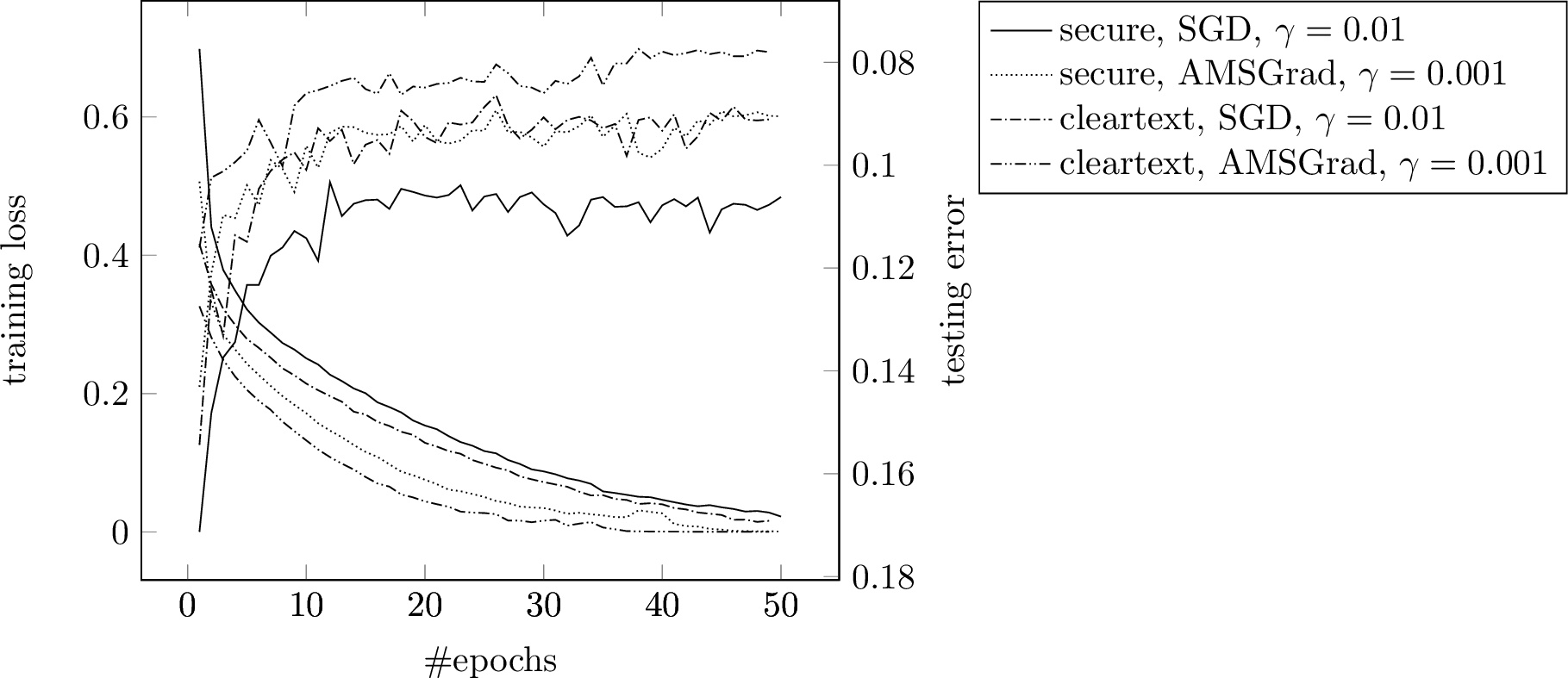
Figure [fig:comp] compares the performance of our secure training with cleartext training in TensorFlow. It shows that secure training performs only slightly worse with the same optimizer.
5.2 CIFAR-10 Classification↩︎
In order to highlight the generality of our approach, we have implemented training for CIFAR-10 with a network by [5], which is based on AlexNet [38]. See Figure 13 in Appendix 11 for details. Unlike the networks for MNIST, the network for CIFAR-10 uses batch normalization [25]. Table 3 shows our results. Our results are not comparable with [5] because they do not implement the full training. Furthermore, [8] do not provide accuracy figures for training from scratch, which makes it unclear how their less accurate approximations perform in this setting. Figure [fig:comp-cifar10] in Appendix 13 shows that our secret training comes within a few percentage points of cleartext training. Similar figures for MPC training on CIFAR-10 are not widely seen in the literature.
| Network | s/ep. | GB/ep. | Acc. | \(f\) |
|---|---|---|---|---|
| [5]\(^*\) | 3,156 | 80 | N/A | 13 |
| [8] | 1,137 | 535 | N/A | 20 |
| Ours (SGD) | 1,603 | 771 | 64.9% | 16 |
| Ours (Adam) | 2,431 | 3,317 | 64.7% | 16 |
| Ours (AMSGrad) | 2,473 | 3,285 | 63.6% | 16 |
6 Conclusions↩︎
We implement deep neural network training purely in multi-party computation, and we present extensive results of convolutional neural networks on benchmark datasets. We find that the low precision of MPC computation increases the error slightly. We only consider one particular implementation of division and exponentiation, which are crucial to the learning process as part of softmax. Future work might consider different approximations of these building blocks.
7 An Efficient Secure Three-Party Computation Protocol↩︎
There is a wide range of MPC protocols with a variety of security properties (see [9] for an overview). In this section, we focus on the setting of three-party computation with one semi-honest corruption. This means that, out of the three parties, two are expected to behave honestly, i.e., they follow the protocol and keep their view of the protocol secret, and one party is expected to follow the protocol but might try to extract information from their view. The reason for choosing this setting is that it allows for an efficient MPC protocol while still providing secure outsourced computation. The protocol does not easily generalize to any other setting. However, protocols exist for any number of parties, see Keller for an overview. The concrete protocol we use goes back to [39] with further aspects by [40], [3], and [41]. We summarize the core protocol below. The mathematical building blocks in the next section mostly use the aspects below.
7.0.0.1 Secret sharing
The simplest variant of secure computation is only data-oblivious, that is, the participants are aware of the nature of the computation (addition, multiplication, etc.) but not the values being operated on. In the context of machine learning, this means that they know the hyper-parameters such as the layers but not the sample data or the neural network weights. All of these values in our protocol are stored using replicated secret sharing. A secret value \(x\) is a represented as a random sum \(x = x_0 + x_1 + x_2\), and party \(P_i\) holds \((x_{i-1}, x_{i+1})\) where the indices are computed modulo three. Clearly, each party is missing one value to compute the sum. On the other hand, each pair of parties hold all necessary to reconstruct the secret. For a uniformly random generation of shares, the computation domain has to be finite. Most commonly, this domain is defined by integer computation modulo a number. We use \(2^k\) for \(k\) being a multiple of 64 as well as 2 as the moduli. The first case corresponds to an extension of 64-bit arithmetic found on most processors. We will refer to the two settings as arithmetic and binary secret sharing throughout the paper.
7.0.0.2 Input sharing
The secret sharing scheme implies a protocol to share inputs where the inputting party samples the shares and distributes them accordingly. [41] propose a more efficient protocol where the inputting party only needs to send one value instead of two pairs of values. If \(P_i\) would like to input \(x\), \(x_i\) is set to zero, and \(x_{i-1}\) is generated with a pseudo-random generator using a key previously shared between \(P_i\) and \(P_{i+1}\). \(P_i\) can compute \(x_{i+1} = x - x_{i-1}\) and send it to \(P_{i-1}\). While the resulting secret sharing is not entirely random, the fact that \(P_i\) already knows \(x\) makes randomizing \(x_i\) obsolete.
7.0.0.3 Addition, subtraction, and scalar multiplication
The commutative nature of addition allows to add secret sharings without communication. More concretely, secret sharings \(x = x_0 + x_1 + x_2\) and \(y = y_0 + y_1 + y_2\) imply the secret sharing \(x + y = (x_0 + y_0) + (x_1 + y_1) + (x_2 + y_2)\). The same works for subtraction. Furthermore, the secret sharing \(x = x_0 + x_1 + x_2\) allows to compute \(\lambda x = \lambda x_0 + \lambda x_1 + \lambda x_2\) locally.
7.0.0.4 Multiplication
The product of \(x = x_0 + x_1 + x_2\) and \(y = y_0 + y_1 + y_2\) is \[\begin{align} x \cdot y &= (x_0 + x_1 + x_2) \cdot (y_0 + y_1 + y_2) \\ &= (x_0y_0 + x_0y_1 + x_1y_0) + (x_1y_1 + x_1y_2 + x_2y_1) + (x_2y_2 + x_2y_0 + x_0y_2). \end{align}\] On the right-hand side (RHS), each term in parentheses only contains shares known by one of the parties. They can thus compute an additive secret sharing (one summand per party) of the product. However, every party only holding one share does not satisfy the replication requirement for further multiplications. It is not secure for every party to pass their value on to another party because the summands are not distributed randomly. This can be fixed by rerandomization: Let \(xy = z_0 + z_1 + z_2\) where \(z_i\) is known to \(P_i\). Every party \(P_i\) computes \(z_i' = z_i + r_{i,i+1} - r_{i-1,i}\) where \(r_{i,i+1}\) is generated with a pseudo-random generator using a key pre-shared between \(P_i\) and \(P_{i+1}\). The resulting sum \(xy = z_0' + z_1' + z_2'\) is pseudo-random, and it is thus secure for \(P_i\) to send \(z_i'\) to \(P_{i+1}\) in order to create a replicated secret sharing \(((xy)_{i-1}, (xy)_{i+1}) = (z_i', z_{i-1}')\).
7.0.0.5 Domain conversion
Recall that we use computation modulo \(2^k\) for \(k\) being a multiple of 64 as well as 1. Given that the main operations are just addition and multiplication in the respective domain, it is desirable to compute integer arithmetic in the large domain but operations with a straight-forward binary circuit modulo two. There has been a long-running interest in this going back to least [42]. We mainly rely on the approach proposed by [3] and [43]. Recall that \(x \in 2^k\) is shared as \(x = x_0 + x_1 + x_2\). Now let \(\{x_0^{(i)}\}_{i=0}^{k-1}\) the bit decomposition of \(x_0\), that is, \(x_0^{(i)} \in \{0,1\}\) and \(x_0 = \sum_{i=0}^{k-1} x_0^{(i)} 2^i\). It is self-evident that \(x_0^{(i)} = x_0^{(i)} + 0 + 0\) is a valid secret sharing modulo two (albeit not a random one). Furthermore, every party holding \(x_0\) can generate \(x_0^{(i)}\). It is therefore possible for the parties to generate a secret sharing modulo two of a single share modulo \(2^k\). Repeating this for all shares and computing the addition as a binary circuit allow the parties to generate a secret sharing modulo two from a secret sharing modulo \(2^k\). Conversion in the other direction can be achieved using a similar technique or using “daBits” described by [44]. In the following, we will use the term mixed-circuit computation for any technique that works over both computation domains.
7.0.0.6 Dot products
Dot products are an essential building block of linear computation such as matrix multiplication. In light of quantization, it is possible to reduce the usage of truncation by deferring it to after the summation. In other words, the dot product in the integer representations is computed before truncating. This not only reduces the truncation error, but also is more efficient because the truncation is the most expensive part in quantized secure multiplication. Similarly, our protocol allows to defer the communication needed for multiplication. Let \(\vec{x}\) and \(\vec{y}\) be two vectors where the elements are secret-shared, that is, \(\{x^{(i)}\} = x_0^{(i)} + x_1^{(i)} + x_2^{(i)}\) and similarly for \(y^{(i)}\). The inner product then is \[\begin{align} \sum_i x^{(i)} \cdot y^{(i)} &= \sum_i (x_0^{(i)} + x_1^{(i)} + x_2^{(i)}) \cdot (y_0^{(i)} + y_1^{(i)} + y_2^{(i)}) \\ &= \sum_i (x_0^{(i)}y_0^{(i)} + x_0^{(i)}y_1^{(i)} + x_1^{(i)}y_0^{(i)}) + \sum_i (x_1^{(i)}y_1^{(i)} + x_1^{(i)}y_2^{(i)} + x_2^{(i)}y_1^{(i)}) \\ &\quad + \sum_i (x_2^{(i)}y_2^{(i)} + x_2^{(i)}y_0^{(i)} + x_0^{(i)}y_2^{(i)}). \end{align}\] The three sums in the last term can be computed locally by one party each before applying the same protocol as for a single multiplication.
7.0.0.7 Comparisons
Arithmetic secret sharing does not allow to access the individual bits directly. It is therefore not straightforward to compute comparisons such as “less than”. There is a long line of literature on how to achieve this going back to at least [45]. More recently, most attention has been given to combining the power of arithmetic and binary secret sharing in order to combine the best of worlds. One possibility to do so is to plainly convert to the binary domain and compute the comparison circuit there. In our concrete implementation, we use the more efficient approach by [3]. It starts by taking the difference between the two inputs. Computing the comparison then reduces to comparing to zero, which in turn is equivalent to extracting the most significant bit as it indicates the sign. The latter is achieved by converting the shares locally to bit-wise sharing of the arithmetic shares, which sum up to the secret value. It remains to compute the sum of the binary shares in order to come up with the most significant bit.
7.0.0.8 Shifting and truncation
[31] present an efficient implementation of the deterministic truncation using mixed-circuit computation, and [46] present an efficient protocol for the probabilistic truncation.
The probabilistic truncation involves the truncation of a randomized value, that is the computation of \(\lfloor (x+r)/2^f \rfloor\) for a random \(f\)-bit value \(r\). It is easy to see that \[\lfloor (x+r)/2^f \rfloor = \begin{cases} \lfloor x/2^f \rfloor & \text{if }(x \bmod 2^f + r) < 2^f \\ \lfloor x/2^f \rfloor + 1 & \text{otherwise.} \end{cases}\] Therefore, the larger \((x \bmod 2^f)\) is, the more likely the latter condition is true.
8 An Efficient Multi-Party Computation Protocol Based on Homomorphic Encryption↩︎
While the protocol in the previous is very efficient, the multiplication only works with an honest majority, that is, the number of corrupted parties is strictly less than half of the total number. Multiplications with more corruptions than that requires more involved cryptographic schemes. In this section, we present a semi-honest protocol based on homomorphic encryption that tolerates \(n-1\) corrupted parties out of \(n\).
8.0.0.1 Secret sharing
The simplest secret sharing is additive secret sharing, which can be used in this setting. The share of party \(i\) is a random element \(x_i\) of the relevant domain such that the sum of all elements is the secret.
8.0.0.2 Input sharing
The canonical input sharing would be for the inputting party to generate random shares such that they add up to the input and then distribute the shares. Using a one-time setup, it is possible to share without communication as shown in Algorithm 5. It is easy to see that the resulting sharing is correct and that the unknown shares are indistinguishable to random for an adversary corrupting any number of parties.

8.0.0.3 Addition, subtraction, and scalar multiplication
As with any linear secret sharing scheme, these operation can trivially be computed locally.
8.0.0.4 Multiplication
We use Beaver’s technique [47]. Assume that \(a\) and \(b\) are random numbers in the domain, and \(c=ab\). Then, for any \(x, y\), it holds that \[\begin{align} xy &= (x + a - a) \cdot (y + b - b) \\ &= (x + a) \cdot (y + b) - (y + b) \cdot a - (x + a) \cdot b + c. \end{align}\] As \(a\) and \(b\) and random, they can be used to used to mask \(x\) and \(y\), respectively. Once \(x+a\) and \(y+b\) have been revealed, the operation becomes linear in \(a\) and \(b\): \[[xy] = (x + a) \cdot (y + b) - (y + b) \cdot [a] - (x + a) \cdot [b] + [c]\]
It remains to produce a fresh triple \((a, b, c)\) for every multiplication. [48] show how to do this using semi-homomorphic encryption based on Learning With Errors (LWE), a widely used cryptographic assumption. They make optimal use of the SIMD (single instruction, multiple data) nature of LWE-based encryption. Their protocol involves pair-wise communication between parties, which scale quadratically in the number of parties. In the following section, we propose a protocol that scales better, which is inspired by [49].
8.0.0.5 Matrix multiplication
[50] have extended Beaver’s technique to matrix multiplication by replacing \(x, a\) with \(m \times n\) and \(y, b\) with \(n \times p\) matrices. Using the diagonal packing by [51] allows to implement the matrix triple generation with \(O(m (n + l))\) communication instead of the naïve \(O(mnl)\). Unlike Halevi and Shoup, we only use the semi-homomorphic encryption, that is, only public-private multiplications. This avoids the need for cycling or shifting because we can simply generate the necessary cleartexts as needed.
8.0.0.6 Domain conversion
daBits [44] and edaBits [32] are a generic method to convert between integer and binary computation. For the special case of semi-honest two-party computation, [52] have presented a more efficient protocol similar to the one in the previous section.
8.0.0.7 Comparison, shifting, and truncation
[32] have shown how to use edaBits to implement these computations. Essentially, they make minimal use of binary computation before switching back to integer computation so that the result is available for further computation in the integer domain.
8.1 Linear-cost Triple Generation with Semi-homomorphic Encryption↩︎
Assume an encryption system that allows to multiply a ciphertext and a plaintext, that is, \(\mathsf{Dec}(\mathsf{Enc}(\mathbf{a}) \cdot \mathbf{b}= \mathbf{a}* \mathbf{b}\) where \(\mathbf{a}\) and \(\mathbf{b}\) are vectors and \(*\) denotes the Schur product. LWE allows the efficient creation of such a system. Furthermore, assume a distributed key setup as used by [53]. Since we only want to achieve semi-honest security, it is straight-forward to generate without using any protocol to check the correctness. Algorithm 6 show the details of our protocol.

By definition, \[\begin{align} \sum \mathbf{c}_i &= \mathsf{Dec}(C_c) \\ &= \mathsf{Dec}(\sum_i C_a * \mathbf{b}_i + \mathsf{Enc}(0)) \\ &= \mathsf{Dec}(C_a * \sum_i \mathbf{b}_i) \\ &= \mathsf{Dec}(\sum_i \mathsf{Enc}(\mathbf{a}_i) * \sum_i \mathbf{b}_i) \\ &= (\sum_i \mathbf{a}_i) * (\sum_i \mathbf{b}_i). \end{align}\] This proves correctness. Furthermore, the distributed key setup hides encrypted values from all parties, and the addition of \(\mathsf{Enc}(0)\) in step [step:mult] ensures that \(P_1\) only receives a fresh encryption of \(\mathbf{a}* \mathbf{b}_i\).
8.2 Replacing Homomorphic Encryption by a Dealer↩︎
It is possible to generate all correlated randomness (triples, random bits, (e)daBits etc.) by one party. The security then relies on the fact that either the dealer is trusted or all of the remaining parties. The offline phase simply consists of the dealer generating the necessary randomness (for example, a random triple \((a, b, ab)\)) and then sending an additive secret sharing to the remaining parties.
9 High-Level Secure Computation Building Blocks↩︎
In this section, we will discuss how to implement computation with MPC with a focus on how it differs from computation on CPUs or GPUs. Most of the techniques below are already known individually. To the best of our knowledge, however, we are the first to put them together in an efficient and extensible framework for secure training of deep neural networks.
9.0.0.1 Oblivious Selection
Plain secure computation does not allow branching because the parties would need to be aware of which branch is followed. Conditional assignment can be implemented as follows. If \(b \in \{0,1\}\) denotes the condition, \(x + b \cdot (y - x)\) is either \(x\) or \(y\) depending on \(b\). If the condition is available in binary secret sharing but \(x\) and \(y\) in arithmetic secret sharing, \(b\) has to be converted to the latter. This can be done using a daBit [44], which is a secret random bit shared both in arithmetic and binary. It allows to mask a bit in one world by XORing it. The result is then revealed and the masking is undone in the other world.
9.0.0.2 Division
[20] show how to implement quantized division using the algorithm by [54]. It mainly uses arithmetic and the probabilistic truncation already explained. In addition, the initial approximation requires a full bit decomposition as described above. The error of the output depends on the error in the multiplications used for Goldschmidt’s iteration, which compounds in particular when using probabilistic truncation. Due to the nature of secure computation, the result of division by zero is undefined. One could obtain a secret failure bit by testing the divisor to zero. However, that is unnecessary in our algorithm, because so far we only use division by secret value for the softmax function, where the divisor is guaranteed to strictly positive.
9.0.0.3 Logarithm
Computation logarithm with any public base can be reduced to logarithm to base two using \(\log_x y = \log_2 y \cdot \log_x 2\). [22] propose to represent \(y\) as \(y = a \cdot 2^b\), where \(a \in [0.5,1)\) and \(b \in \mathbb{Z}\). This then allows to compute \(\log_2 y = \log_2 a + b\). Given the restricted range of \(a\), \(\log_2 a\) can be approximated using a division of polynomials. Numerical stability and input range control are less of an issue here, because we only use logarithm for the loss computation, which does not influence the training.
9.0.0.4 Inverse square root
Secret share \(\langle \tilde{x}; f \rangle^{\mathsf{A}}\) where \(2^{-f+1} \le \tilde{x} \le 2^{f-1}\).
\(\langle \tilde{u}; f \rangle^{\mathsf{A}}\) and \(\langle z_0 \rangle^{\mathsf{B}}, \dots, \langle z_{k-1} \rangle^{\mathsf{B}}\) such that \(z_{e+f} = 1\), \(z_i = 0\) for \(i \ne e+f\), and \(\tilde{u} = \tilde{x}^{-1} \cdot 2^{e+1} \in [0.25,0.5)\).
\(\langle z_0 \rangle^{\mathsf{B}}, \dots, \langle z_{k-1} \rangle^{\mathsf{B}} \leftarrow\mathsf{NP2}(\langle \tilde{x}; f \rangle^{\mathsf{A}})\) \(\langle 2^{e-1}; f \rangle^{\mathsf{A}} \leftarrow\mathsf{B2A}(\langle z_{2f-1} \rangle^{\mathsf{B}}, \dots, \langle z_0 \rangle^{\mathsf{B}})\) \(\langle \tilde{u}; f \rangle^{\mathsf{A}} \leftarrow\langle \tilde{x}; f \rangle^{\mathsf{A}} \cdot \langle 2^{e-1}; f \rangle^{\mathsf{A}}\) return \(\langle \tilde{u}; f \rangle^{\mathsf{A}}, (\langle z_0 \rangle^{\mathsf{B}}, \dots, \langle z_{k-1} \rangle^{\mathsf{B}}\)
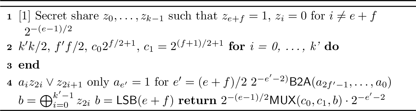

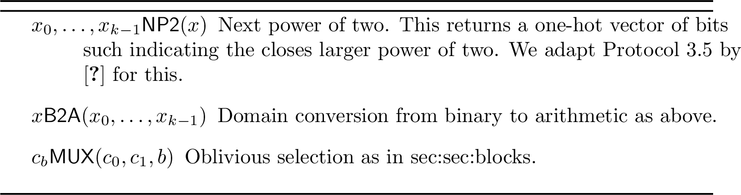
Figure 7: Procedures in Algorithms [alg:sep]–7 (b). a — Square-root compensation (\(\mathsf{SqrtComp}\)), b — \(\mathsf{InvertSqrt}\) [29], c — Procedures in Algorithms [alg:sep]–7 (b)
[22] propose to compute square root using Goldschmidt and Raphson-Newton iterations. We could combine this with the division operator introduced above. However, [29] propose a more direct computation that avoids running two successive iterations. We have optimized their algorithm \(\mathsf{SqrtComp}\) computing the square root of a power of two as shown in Algorithm 7 (a). As an essential optimization, we compute the least significant bit of \(e+f\) by simply XORing every other \(z_i\) in step [step:lsb] of Algorithm 7 (a). Given that XOR does not require communication with binary secret sharing, this is much more efficient than computing the least significant bit of a sum of oblivious selections done by [29] Remarkably, our optimization cuts the cost by roughly half. This is due to the reduction in conversions from binary to arithmetic. Furthermore, we correct some issues which result in outputs that are off by a multiplication with a power of two. We present the rest of their approach in Algorithms [alg:sep] and 7 (b) (unchanged) for completeness. Unlike [29], we do not explicitly state the truncation after fixed-point multiplication.
| 3 Parties | 2 Parties | |||
| SH | Mal. | SH | Mal. | |
| [29] | 19 | 160 | 481 | 25,456 |
| Ours | 9 | 114 | 342 | 21,522 |
Table 4 shows how our approach compares to [29]. In the context of the Figures in Table [tbl:table:sec-models], this implies an improvement of up one quarter. The importance of inverse square root stems from the fact that it is computed for every iteration and trainable parameter in the parameter update.
9.0.0.5 Uniformly random fractional number
Limiting ourselves to intervals of the form \([x, x + 2^e)\) for a potentially negative integer \(e\), we can reduce the problem to generate a random \((f + e)\)-bit number where \(f\) is the fixed-point precision. Recall that we represent a fractional number \(x\) as \(\lfloor x \cdot 2^{-f} \rceil\). Generating a random \(n\)-bit number is straightforward using random bits, which in our protocol can be generated as presented by [55]. However, [31] and [32] present more efficient approaches that involve mixed-circuit computation.
9.0.0.6 Communication cost
Table 5 shows the total communication cost of some of the building blocks in our three-party protocol for \(f=16\). This setting mandates the modulus \(2^{64}\) because the division protocol requires a bit length of \(4f\).
| Bits | |
|---|---|
| Integer multiplication | 192 |
| Probabilistic truncation | 960 |
| Nearest truncation | 2,225 |
| Comparison | 668 |
| Division (prob. truncation) | 10,416 |
| Division (nearest truncation) | 24,081 |
| Exponentiation (prob. truncation) | 16,303 |
| Exponentiation (nearest truncation) | 43,634 |
| Invert square root (prob. truncation) | 9,455 |
| Invert square root (nearest truncation) | 15,539 |
10 Deep Learning Building Blocks↩︎
In this section, we will use the building blocks in Appendix 9 to construct high-level computational modules for deep learning.
10.0.0.1 Fully connected layers
Both forward and back-propagation of fully connected layers can be seen as matrix multiplications and thus can be implemented using dot products. A particular challenge in secure computation is to compute a number of outputs in parallel in order to save communication rounds. We overcome this challenge by having a dedicated infrastructure in our implementation that computes all dot products for a matrix multiplication in a single batch of communication, thus reducing the number of communication rounds.
10.0.0.2 2D convolution layers
Similar to fully connected layers, 2D convolution and its corresponding gradient can be implemented using only dot products, and we again compute several output values in parallel.
10.0.0.3 ReLU
Given the input \(x\in\mathbb{R}\), a rectified linear unit (ReLU [24]) outputs \[\mathsf{ReLU}(x) \mathrel{\mathop{:}}= \max(x,0) = \iverson{x>0} \cdot x.\]
It can thus be implemented as a comparison followed by an oblivious selection. For back-propagation, it is advantageous to reuse the comparison results from forward propagation due to the relatively high cost of secure computation. Note that the comparison results are stored in secret-shared form and thus there is no reduction in security.
10.0.0.4 Max pooling
Similar to ReLU, max pooling can be reduced to comparison and oblivious selection. In secure computation, it saves communication rounds if the process uses a balanced tree rather than iterating over all input values of one maximum computation. For example, two-dimensional max pooling with a 2x2 window requires computing the maximum of four values. We compute the maximum of two pairs of values followed by the maximum of the two results. For back-propagation, it again pays off to store the intermediate results from forward propagation in secret-shared form.
10.0.0.5 Dropout
Dropout layers [30] require generating a random bit according to some probability and oblivious selection. For simplicity, we only support probabilities that are a power of two.
10.0.0.6 Batch normalization
As another widely used deep learning module, batch normalization (BN, [25]). Based on a mini-batch \(\mathcal{B}=\{x_i\}\) of any input statistic \(x\), the BN layer outputs \[\begin{align} y_i = \gamma \frac{x_i-\mu_{\mathcal{B}}}{\sqrt{\sigma_{\mathcal{B}}^2}+\epsilon} + \beta, \end{align}\] where \(\mu_{\mathcal{B}}\) and \(\sigma^2_{\mathcal{B}}\) are the first and second central moments of \(x\), and \(\gamma\), \(\beta\) and \(\epsilon\) are hyper-parameters. In addition to basic arithmetic, it requires inverse square root, which is not trivial in MPC.
10.0.0.7 Softmax output and cross-entropy loss
For classification tasks, consider softmax output units \(\frac{\exp({x}_i)}{\sum_j \exp(x_j)}\), where \(\boldsymbol{x}=(x_1,x_2,\cdots)\) is the linear output (logits) of the last layer, and the cross-entropy loss \(\ell= - \sum_{i} y_i \log \frac{\exp({x}_i)}{\sum_j \exp(x_j)} = - \sum_{i} x_iy_i + \log\sum_{j} \exp( x_j )\), where \(\boldsymbol{y}=(y_1,y_2,\cdots)\) is the ground truth one-hot vector. This usual combination requires computing the following gradient for back-propagation: \[\begin{align} \label{eq:grad} \bigtriangledown_i \mathrel{\mathop{:}}= \frac{\partial\ell}{\partial x_i}&= \frac{\partial}{\partial x_i} \Big( -\sum_k y_k \cdot x_k + \log \sum_j \exp( x_j ) \Big)\nonumber\\ &= -y_i + \frac{\exp(x_i)}{\sum_j \exp(x_j)}. \end{align}\tag{2}\]
On the RHS of the above eq. (2 ), the values in the denominator are potentially large due to the exponentiation. This is prone to numerical overflow in our quantized representation, because the latter puts strict limits on the values. We therefore optimize the computation by first taking the maximum of the input values: \(x_{\max} = \max_i x_i\). Then we evaluate \(\bigtriangledown_i\) based on \[\bigtriangledown_i = \frac{\exp(x_i-x_{\max})}{\sum_j \exp(x_j-x_{\max})} - y_i.\] As \(\forall{j}\), \(x_j\le{}x_{\max}\), we have \(1 \le \sum_j \exp(x_j-x_{\max})\le L\), where \(L\) is the number of class labels (\(L=10\) for MNIST). Hence numerical overflow is avoided. The same technique can be used to compute the sigmoid activation function, as \(\mathrm{sigmoid}(x) \mathrel{\mathop{:}}=\frac{1}{1+\exp(-x)} = \frac{\exp(0)}{\exp(0)+\exp(-x)}\) is a special case of softmax.
10.0.0.8 Stochastic gradient descent
The model parameter update in SGD only involves basic arithmetic: \[\label{eq:sgd} \theta_j \leftarrow \theta_j - \frac{\gamma}{B} \sum_{i=1}^B \frac{\partial\ell_i}{\partial\theta_j},\tag{3}\] where \(\theta_j\) is the parameter indexed by \(j\), \(\gamma>0\) is the learning rate, \(B\) is the mini-batch size, \(\ell_i\) is the cross-entropy loss with respect to the \(i\)’th sample in the mini-batch. To tackle the limited precision with quantization, we defer dividing by the batch size \(B\) to the model update in eq. (3 ). In other words, the back-propagation computes the gradient \(\frac{\partial\ell_i}{\partial\theta_j}\), where the back-propagated error terms are not divided by \(B\). Division by the batch size \(B\) only happens when the parameter update is performed. Since the batch size is a power of two (128), it is sufficient to use probabilistic truncation instead of full-blown division. This both saves time and decreases the error.
10.0.0.9 Adam [26] and AMSGrad [27]
Optimizers in this category perform a more sophisticated parameter update rule5: \[\theta_j \leftarrow \theta_j - \frac{\gamma}{\sqrt{v_j + \epsilon}} g_j,\] where \(\epsilon>0\) is a small constant to prevent division by zero, and \(g_j\) and \(v_j\) are the first and second moments of the gradient \(\frac{\partial\ell}{\partial\theta_j} =\frac{1}{B}\sum_{i=1}^B \frac{\partial\ell_i}{\partial\theta_j}\), respectively. Division by the batch size \(B\) can be skipped in computing \(\frac{\partial\ell}{\partial\theta_j}\), because scaling of the gradient leads to the same scaling factor of \(g_j\) and \(\sqrt{v_j}\). Both \(g_j\) and \(v_j\) are computed from the back-propagation result using simple arithmetic and comparison (in the case of AMSGrad). We compute the inverse square root as described in Section 9 above.
10.0.0.10 Parameter initialization
We use the widely adopted initialization method proposed by [28]. Each weight \(w\) between two layers with size \(d_{\mathrm{in}}\) and \(d_{\mathrm{out}}\) is initialized by \[w\sim \mathcal{U}\left[-\sqrt{\frac{6}{d_{\mathrm{in}}+d_{\mathrm{out}}}}, \sqrt{\frac{6}{d_{\mathrm{in}}+d_{\mathrm{out}}}}\right],\] where \(\mathcal{U}[a, b]\) means the uniform distribution in the given range \([a,b]\). Besides basic operations, it involves generating a uniformly distributed random fractional value in a given interval, which is introduced in the previous section 9. All bias values are initialized to 0.
11 Models↩︎
The neural network structures investigated in this paper are given by the following Figures 8, 9, 10, 11 and 13. The structure of each network is formatted in Keras6 code.
![Figure 8: Network A used by [2]](/article/2107.00501/_pdflatex/gmwprzdv.png "fig:")
![Figure 9: Network B used by [36]](/article/2107.00501/_pdflatex/ghslxudr.png "fig:")
![Figure 10: Network C used by [13] (with optional Dropout layer)](/article/2107.00501/_pdflatex/imanojur.png "fig:")
![Figure 11: Network D used by [37]](/article/2107.00501/_pdflatex/vlbitfcx.png "fig:")
Figure 12: 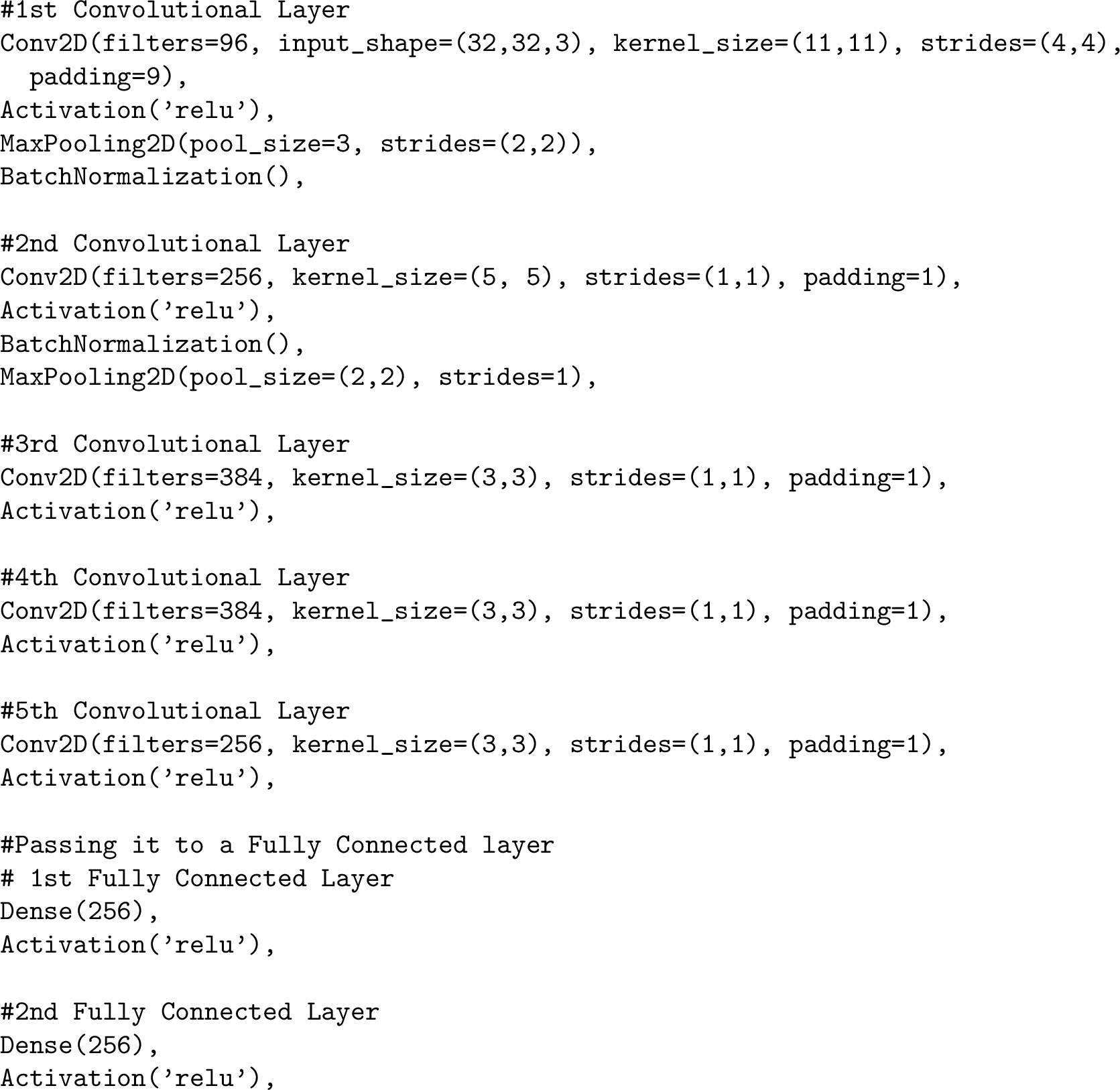 .
.
![Figure 13: AlexNet for CIFAR-10 by [5]. Note that our implementation allows any padding unlike Keras.](/article/2107.00501/_pdflatex/duxcnhjk.png "fig:")
12 Fashion MNIST↩︎
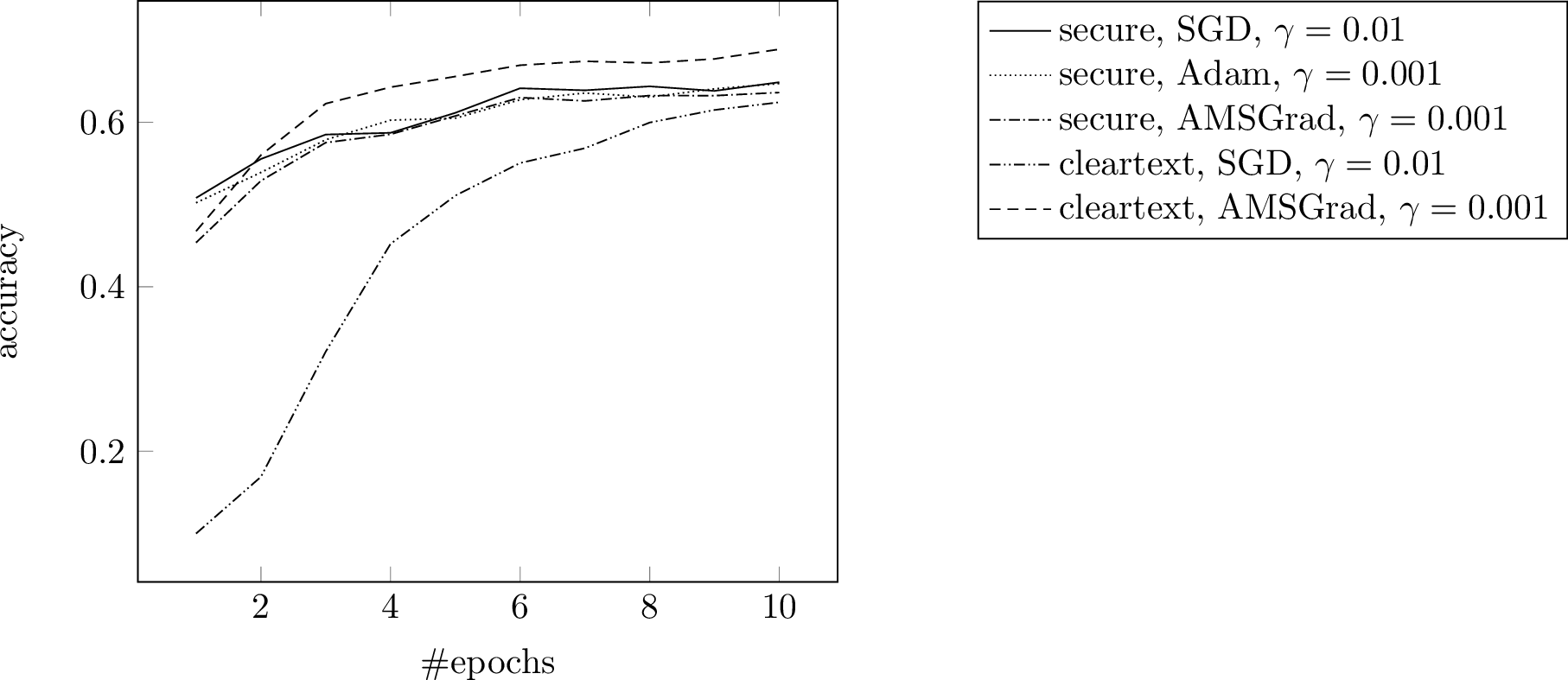
We run our implementation on Fashion MNIST [56] for a more complete picture. Figure 14 shows our results. See [56] for an overview on how other models perform in cleartext.
13 More Experimental Results↩︎
For the task of classifying MNIST digits, Figure [fig:nets] shows the learning curves for all networks used by [4]. Among all the investigated structures, LeNet (network C) performs the best. Furthermore, AMSGrad consistently improves the classification performance as compared to SGD.
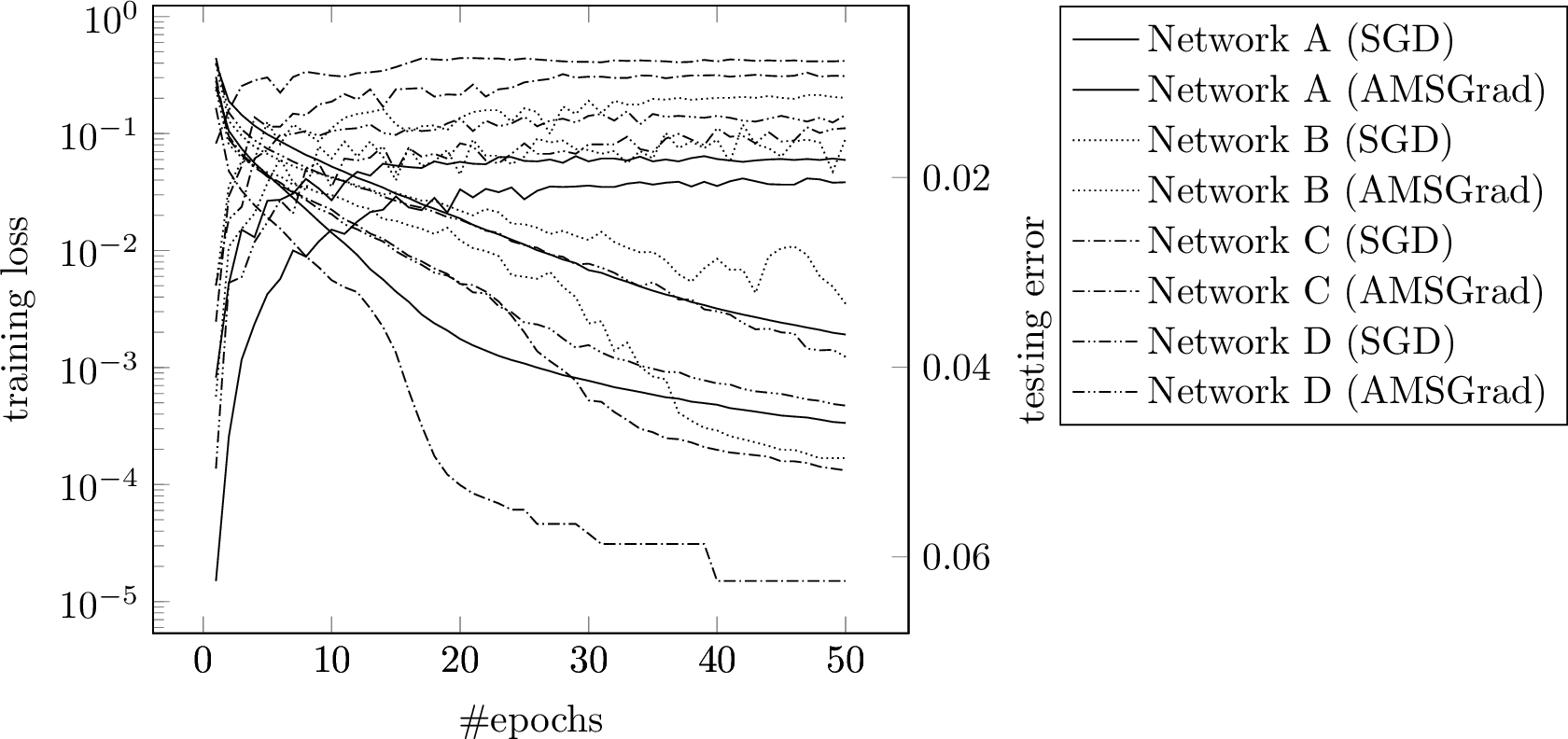
Figure [fig:comp-cifar10] shows the comparison of cleartext training and secure training for CIFAR-10 with \(f=16\) and probabilistic truncation. Our MPC implementation has gained similar performance with the cleartext counterpart.
14 Hyperparameter Settings↩︎
In the following we discuss our choice of hyperparameters.
- Number of epochs
-
As we found convergence after 100 epochs, we have run most of our benchmarks for 150 epochs, except for the comparison of optimizers where we stopped at 100.
- Early stop
-
We have not used early stop.
- Mini-batch size
-
We have used 128 throughout as it is a standard size. We briefly trialed 1024 as suggested by [57], but did not found any improvement.
- Reshuffling training samples
-
At the beginning of each epoch, we randomly re-shuffle the training samples using the Fisher-Yates shuffle with MP-SPDZ’s internal pseudo-random number generator as randomness source.
- Learning rate
-
We have tried a number of learning rates as documented in Figure 4. As a result, we settled for 0.01 for SGD and 0.001 for AMSGrad in further benchmarks.
- Learning rate decay/schedule
-
We have not used either.
- Random initialization
-
The platform uses independent random initialization by design.
- Dropout
-
We have experimented with Dropout but not found any improvement as shown in Figure 4.
- Input preprocessing
-
We have normalized the inputs to \([0, 1]\).
- Test/training split
-
We have used the usual MNIST split.
- Hyperparameters for Adam/AMSGrad
-
We use the common choice \(\beta_1 = 0.9\), \(\beta_2 = 0.999\), and \(\epsilon = 10^{-8}\).
15 List of Symbols↩︎
| \(\Re\) | the set of real numbers |
| \(\Ze\) | the set of integers |
| \(x\), \(y\), \(\lambda\) | real numbers in \(\Re\) |
| \(\bm{x}\), \(\bm{y}\) | real vectors |
| \(\round{x}\) | nearest rounding of \(x\): \(\round{x}\defeq\argmin_{z\in\Ze} \vert{}x-z\vert\) |
| \(\floor{x}\) | floor function: \(\floor{x}\defeq\max\{z\in\Ze\,\vert\,z\le{x}\}\) |
| \(\{x\}\) | the fractional part of \(x\): \(\{x\}\defeq{}x-\floor{x}\) |
| \(Q^f(x)\) | the integer representation of \(x\): \(Q^f(x)=\round{x\cdot2^f}\) |
| \(\uniform(a,b)\) | uniform distribution on \([a,b]\) |
| \(\bernoulli(p)\) | Bernoulli distribution (with probability \(p\) the random variable equals \(1\)) |
| \(\iverson{c}\) | Iverson bracket (\(\iverson{c}=1\) if \(c\) is true otherwise 0) |
| \(\vert\cdot\vert\) | absolute value |
| \(\Vert\cdot\Vert\) | Frobenius norm |
| \(\mathrm{Prob}(\cdot)\) | probability of the parameter statement being true |
| \((\mathrm{condition}~?~a~:~b)\) | oblivious selection |
16 Proofs↩︎
16.1 Proof of Proposition 1↩︎
Proof. By Eq. (1 ), \[E(b) = 0 \times (1-\{\mu\}) + 1 \times \{\mu\} = \{\mu\}.\] Therefore \[\begin{align} E(R^f(xy)) &= E( \lfloor \mu \rfloor + b ) = \lfloor \mu \rfloor + E(b) = \lfloor \mu \rfloor + \{\mu\} = \lfloor \mu \rfloor + (\mu-\lfloor \mu \rfloor) = \mu = Q^f(x) Q^f(y) 2^{-f}. \end{align}\] Notice that \(Q^f(A)\) is simply obtained through entry-wise quantization \(Q^f(a_{ij})\). By our matrix multiplication algorithm, \[\begin{align} E(R_{ij}^f(AB)) &= E\left(\sum_{k}R^f(A_{ik}B_{kj})\right)\nonumber\\ &= \sum_{k} E( R^f(A_{ik}B_{kj}) ) \nonumber\\ &= \sum_{k} Q^f(A_{ik}) Q^f(B_{kj}) 2^{-f} \nonumber\\ &= 2^{-f} \sum_{k} Q_{ik}^f(A) Q_{kj}^f(B_{kj}) \nonumber\\ &= 2^{-f} ( Q^f(A) Q^f(B) )_{ij}. \end{align}\] In matrix form, it gives \[E(R^f(AB)) = 2^{-f} Q^f(A) Q^f(B).\] ◻
16.2 A Lemma of Probabilistic Rounding↩︎
Lemma 1. Given \(x,y\in(-2^k,2^k)\subset\mathbb{R}\), \[\begin{align} \left\vert xy - R^f(xy) 2^{-f} \right\vert & < (\max\{\vert{}x\vert,\vert{}y\vert\} + 1)\epsilon + \epsilon^2/4 < (2^k+1) \epsilon + \epsilon^2/4, \end{align}\] where \(\epsilon\mathrel{\mathop{:}}={}2^{-f}\).
Proof. We have \[\vert xy - R^f(xy)2^{-f} \vert \le \vert xy - \mu 2^{-f} \vert + \vert R^f(xy)2^{-f} - \mu 2^{-f}\vert = \vert xy - \mu 2^{-f} \vert + 2^{-f} \vert R^f(xy)- \mu\vert.\] By the definition of \(R^f(xy)\), \[\begin{align} \vert R^f (xy)-\mu \vert = \vert \lfloor \mu \rfloor + b - \mu\vert = \vert b - (\mu-\lfloor \mu \rfloor) \vert = \vert b - \{\mu\} \vert < 1. \end{align}\] Therefore, we have \[\vert xy - R^f(xy)2^{-f} \vert < \vert xy - \mu 2^{-f} \vert + 2^{-f} = \vert xy - \mu 2^{-f} \vert + \epsilon.\] Now we only need to bound the deterministic term \(\vert xy - \mu 2^{-f} \vert\). We have \[\begin{align} \vert xy - \mu 2^{-f} \vert &= \vert xy - Q^f(x) Q^f(y) 2^{-2f} \vert \nonumber\\ &= \vert Q^f(x) Q^f(y) 2^{-2f} - xy \vert \nonumber\\ &= \vert ( Q^f(x) 2^{-f} -x )( Q^f(y) 2^{-f} - y ) + 2^{-f}Q^f(x)y + 2^{-f}Q^f(y)x - 2xy \vert \nonumber\\ &= \vert ( Q^f(x) 2^{-f} -x )( Q^f(y) 2^{-f} - y ) + (2^{-f}Q^f(x)-x)y + (2^{-f}Q^f(y)-y)x \vert \nonumber\\ &\le \vert Q^f(x) 2^{-f} -x \vert \cdot \vert Q^f(y) 2^{-f} - y \vert + \vert 2^{-f}Q^f(x) - x \vert \cdot \vert{}y\vert + \vert 2^{-f}Q^f(y) - y \vert \cdot \vert{}x\vert. \end{align}\] We notice that \(\forall{x}\in\mathbb{R}\), \[\begin{align} \vert 2^{-f}Q^f(x) - x \vert &= \vert 2^{-f}\lfloor x\cdot 2^f \rceil - x \vert = 2^{-f} \vert \lfloor x\cdot 2^f \rceil - x\cdot2^f \vert\nonumber\\ &\le 2^{-f} \times \frac{1}{2} = 2^{-f-1} = \frac{\epsilon}{2}. \end{align}\] Then, we get \[\begin{align} \vert xy - \mu 2^{-f} \vert &\le \frac{\epsilon}{2} \cdot \frac{\epsilon}{2} + \frac{\epsilon}{2} \cdot ( \vert x \vert + \vert y \vert ) = \frac{\epsilon^2}{4} + \frac{\epsilon}{2} \cdot ( \vert x \vert + \vert y \vert )\nonumber\\ &\le \frac{\epsilon^2}{4} + \frac{\epsilon}{2} \cdot ( 2 \max\{\vert{x}\vert, \vert{y}\vert\} ) = \frac{\epsilon^2}{4} + \max\{\vert{x}\vert, \vert{y}\vert\} \epsilon. \end{align}\] In summary, \[\begin{align} \vert xy - R^f(xy)2^{-f} \vert < \vert xy - \mu 2^{-f} \vert + \epsilon \le \frac{\epsilon^2}{4} + \max\{\vert{x}\vert, \vert{y}\vert\} \epsilon +\epsilon = (\max\{\vert{x}\vert, \vert{y}\vert\}+1) \epsilon + \frac{\epsilon^2}{4}. \end{align}\] The second “\(<\)” is trivial by noting our assumption \[\begin{align} \max\{\vert{x}\vert, \vert{y}\vert\} < 2^k. \end{align}\] ◻
16.3 Proof of Proposition 2↩︎
Proof. The proof is based on Lemma 1. \[\begin{align} \Vert AB - R^f(AB) 2^{-f} \Vert &= \sqrt{\sum_{i,j} \left( (AB)_{ij} - R^f_{ij}(AB) 2^{-f} \right)^2} \nonumber\\ &= \sqrt{\sum_{i,j} \left( \sum_{l} A_{il} B_{lj} - \sum_{l} R^f(A_{il}B_{lj}) 2^{-f} \right)^2} \nonumber\\ &= \sqrt{\sum_{i,j} \left\vert \sum_{l} \left(A_{il}B_{lj} - R^f(A_{il}B_{lj}) 2^{-f} \right) \right\vert^2} \nonumber\\ & \le \sqrt{\sum_{i,j} \left( \sum_{l} \left\vert A_{il}B_{lj} - R^f(A_{il}B_{lj}) 2^{-f} \right\vert \right)^2} \nonumber\\ & < \sqrt{\sum_{i,j} \left[ \sum_{l} \left( (2^k+1)\epsilon + \frac{\epsilon^2}{4} \right) \right]^2 } \nonumber\\ & = \sqrt{mp\cdot{}n^2\cdot\left( (2^k+1)\epsilon + \frac{\epsilon^2}{4} \right)^2 } \nonumber\\ & = \sqrt{mp}n\left((2^k+1)\epsilon + \frac{\epsilon^2}{4}\right). \end{align}\] Multiplying both sides by \(2^f\), we get \[\begin{align} \Vert R^f(AB) - 2^{f} A B \Vert < \sqrt{mp}n\left((2^k+1) + \frac{\epsilon}{4}\right). \end{align}\] ◻
16.4 Proof of Proposition 3↩︎
Proof. Note that the variance, denoted as \(\sigma^2(\cdot)\), of \(R^f(xy)\) is \[\begin{align} \sigma^2( R^f(xy) ) &= \sigma^2(b) = E(b^2) - (E(b))^2 = E(b) - (E(b))^2 = \{\mu\} - (\{\mu\})^2 = \{\mu\} (1 - \{\mu\}) \\ &\le \left(\frac{ \{\mu\} + (1 - \{\mu\}) }{2}\right)^2 = \frac{1}{4}. \end{align}\] Therefore, \[\begin{align} \sigma^2( R^f_{ij}(AB) ) &= \sigma^2\left( \sum_k R^f(A_{ik} B_{kj}) \right) = \sum_k \sigma^2\left( R^f(A_{ik} B_{kj}) \right)\\ &\le \sum_k \frac{1}{4} = \frac{n}{4}. \end{align}\] In matrix form, the element-wise variance of the random matrix \(R^f(AB)\) is \[\sigma^2(R^f(AB)) \le \frac{n}{4} \boldsymbol{1}\boldsymbol{1}^\top,\] where \(\boldsymbol{1}\) is the column vector of 1’s. Note all \(mp\) entries in \(R^f(AB)\) are independent. By the Chebyshev inequality, with probability at least \(1-\frac{mp}{\rho}\), the following is true \[\frac{ \Vert R^f(AB) - E(R^f(AB)) \Vert^2 }{n/4} \le \rho,\] which can be re-written as \[\Vert R^f(AB) - E(R^f(AB)) \Vert \le \frac{\sqrt{\rho{n}}}{2}.\] Let \(\iota\mathrel{\mathop{:}}=\frac{1}{2}\sqrt{\frac{\rho}{mp}}\). Then \(\rho=4\iota^2mp\). In conclusion, with probability at least \[1-\frac{mp}{\rho} = 1-\frac{mp}{4\iota^2mp} = 1-\frac{1}{4\iota^2},\] the following is true: \[\Vert R^f(AB) - E(R^f(AB)) \Vert \le \frac{\sqrt{\rho n}}{2} = \frac{\sqrt{4\iota^2mp\cdot{n}}}{2} = \iota\sqrt{mnp}.\] Based on Proposition 1, the statement can be equivalently written as \[\Vert R^f(AB) - 2^{-f}Q^f(A)Q^f(B) \Vert \le \iota \sqrt{mnp}.\] ◻
References↩︎
Code available at https://github.com/data61/MP-SPDZ.↩︎
\(\mathbb{Z}_M = \mathbb{Z}/M\mathbb{Z}\) denotes integer computation modulo \(M\).↩︎
Scripts are available at https://github.com/csiro-mlai/deep-mpc.↩︎
Our implementation is slightly different from the original Adam and AMSGrad, as we put \(\epsilon\) inside the square root. This is because the inverse square root is implemented as a basic operation that can be efficiently computed in MPC.↩︎
https://keras.io↩︎