Language Model Evaluation Beyond Perplexity
May 31, 2021
Abstract
We propose an alternate approach to quantifying how well language models learn natural language: we ask how well they match the statistical tendencies of natural language. To answer this question, we analyze whether text generated from language models exhibits the statistical tendencies present in the human-generated text on which they were trained. We provide a framework—paired with significance tests—for evaluating the fit of language models to these trends. We find that neural language models appear to learn only a subset of the tendencies considered, but align much more closely with empirical trends than proposed theoretical distributions (when present). Further, the fit to different distributions is highly-dependent on both model architecture and generation strategy. As concrete examples, text generated under the nucleus sampling scheme adheres more closely to the type–token relationship of natural language than text produced using standard ancestral sampling; text from LSTMs reflects the natural language distributions over length, stopwords, and symbols surprisingly well.
1 Introduction↩︎
Neural language models1 have become shockingly good at modeling natural language data in recent years [2]–[4]. Thus, to test just how well neural language models capture language NLP researchers have started to look beyond standard evaluation metrics such as perplexity, endeavoring to understand which underlying attributes of human language these models are learning. To this end, a nascent literature has emerged that focuses on probing language models [5], i.e., determining whether models encode linguistic phenomena. For the most part, these works have been limited to analyses of sentence-level phenomenon, such as subject–verb agreement [6] and garden path effects [7] among a myriad of other properties [8], [9].
In this work, we attempt to understand which macro-level phenomena of human language today’s language models reflect. That is, we pose the question: Do neural language models exhibit the statistical tendencies of human language? Phenomena that can be measured at this level provide an alternate view of a model’s comprehension; for example, rather than exploring whether morphological agreement is captured, we look at whether our models learn the trends across a corpus as a whole, e.g., the token rank–frequency (Zipf’s) relationship. In comparison to standard probing techniques, this framework does not require we know a priori how linguistic phenomena should manifest themselves. That is, when there is no law stating the theoretical tendencies of an attribute of natural language or we have reason to believe our language domain does not follow such a law, we can use the statistical tendencies present in empirical data as our baseline. This characteristic both allows us to assess a model’s fit to highly corpus-dependent distributions—like the length distribution—and mitigates the biases introduced by our own preconceptions regarding properties of natural language.2
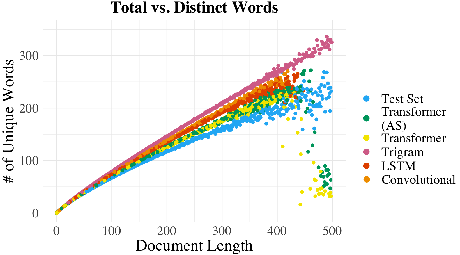
More concretely, our paper describes an experimental design and accompanying hypothesis tests to determine precisely whether text generated from language models follows the same empirical trends as human language. Our experiments reveal that adherence to natural language tendencies varies widely with both model architecture and generation strategy, e.g., 1 shows varying degrees of adherence to the empirical type–token relationship, an artifact that perplexity alone could not reveal. Our findings suggest this framework is a valuable tool for gaining a deeper understanding of where today’s language models are succeeding and failing at capturing human language.
2 Language Models↩︎
Language models are probability distributions over natural language sentences. We define the support of a language model \(p_{\scaleto{{\boldsymbol{\theta}}}{4pt}}\) with parameters \({\boldsymbol{\theta}}\) as \[\mathcal{Y}\mathrel{:\mkern-0.25mu=}\{\mathrm{\small bos}\circ \mathbf{v}\circ \mathrm{\small eos}\mid \mathbf{v}\in \mathcal{V}^* \}\] where \(\mathcal{V}\) is the model’s vocabulary and tokens eos and bos demarcate the beginning and end of a string, respectively, and \(\mathcal{V}^*\) is the Kleene closure of \(\mathcal{V}\). In this paper, we term vocabularies consisting of words closed and those consisting of BPE tokens [10] open.
In the case when \(p_{\scaleto{{\boldsymbol{\theta}}}{4pt}}\) is locally normalized, which is the predominant case for language models, \(p_{\scaleto{{\boldsymbol{\theta}}}{4pt}}\) is defined as the product of probability distributions: \[\label{eq:joint} p_{\boldsymbol{\theta}}(\mathbf{y}) = \prod_{t=1}^{|\mathbf{y}|}p_{\boldsymbol{\theta}}(y_t \mid \mathbf{y}_{<t})\tag{1}\] where each \(p_{\scaleto{{\boldsymbol{\theta}}}{4pt}}(\cdot\! \mid \!\mathbf{y}_{<t})\) is a distribution with support over \(\bar\mathcal{V}\mathrel{:\mkern-0.25mu=}\mathcal{V}\cup \{\mathrm{\small eos}\}\) and \(\mathbf{y}_{<1} = y_0 \mathrel{:\mkern-0.25mu=}\mathrm{\small bos}\). To estimate model parameters \({\boldsymbol{\theta}}\), one typically optimizes the log-likelihood function over a corpus \(\mathcal{C}_{\mathrm{train}}\):
\[\label{eq:lik} \mathcal{L}({\boldsymbol{\theta}}\mid \mathcal{C}_{\mathrm{train}}) = \sum_{\mathbf{y}\in \mathcal{C}_{\mathrm{train}}}\log p_{\scaleto{{\boldsymbol{\theta}}}{4pt}}(\mathbf{y})\tag{2}\] where we call each string \(\mathbf{y}\) a document. To determine the goodness of fit of a model to the empirical distribution (defined by \(\mathcal{C}_{\mathrm{train}}\)), it is standard practice to measure perplexity on a held-out dataset, which is simply a monotonic function of average (per token) log-likelihood under that model. While low perplexity on an evaluation set undoubtedly reflects some level of fit to natural language, it does not give us a fine-grained view of which linguistic attributes a model has learned.
3 Statistical Tendencies of Language↩︎
Human languages are thought to exhibit statistical tendencies, several of which are explicitly quantified by laws [11]. In this section, we review a subset of these distributions–both with and without well-established forms—over which we subsequently perform analyses.
3.1 Classical Laws↩︎
3.1.0.1 Rank–Frequency.
[12]’s law ([12]), otherwise known as the rank–frequency law, states that the frequency of a word in a corpus decays exponentially in the frequency rank of that word, i.e., the frequency \(\omega(\cdot)\) of the \(k^{\text{th}}\) most frequent word \(w_k\) follows the power-law distribution: \(\omega(w_k) \propto k^{-s}\). When fit to natural language text, the free parameter \(s\) is typically close to \(1\). Zipf’s law also has a probabilistic interpretation: the marginal probability that a random word in our corpus takes on the value of the\(k^{\text{th}}\) most frequent can be expressed as
\[\label{eq:zipf} p_{\mathrm{zipf}}(W = w_k) = \frac{1}{\zeta(s)} k^{-s}\tag{3}\] where \(\zeta(s) = 1/\sum_{k=1}^\infty k^{-s}\) is the normalizing constant of our probability mass function (pmf). The adherence of language to Zipf’s law has been widely studied and is considered one of the canonical laws of quantitative linguistics [13]–[15].
Estimating \(s\) from an observed set of rank–frequency pairs can be done using standard estimation techniques. Here we use the maximum-likelihood estimate3 (MLE), employing numerical optimization to solve for \(s\) since the MLE of the discrete power law lacks a closed form solution.
3.1.0.2 Type–Token.
Heaps’ law [18], also known as the type–token relationship, states that the number of additional unique tokens (i.e., number of types) in a document diminishes as its length increases. Formally, we can express the expected number of types \(u(\cdot)\) as a function of the length \(l(\cdot)\) of the string \(\mathbf{y}\) via the relationship \(u(\mathbf{y}) \propto l(\mathbf{y})^\beta\) where \(\beta < 1\) is a free parameter. Types may be, e.g., unigrams or bigrams.
The above formulation of Heaps’ law lacks an obvious probabilistic interpretation. However, if we frame Heaps’ law as modeling the expected value of the number of types for any given length document, then we can model the relation as a Poisson process, where the marginal distribution over document length follows Heaps’ proposed power law. Specifically, we model the number of types for a document of a given length as a non-homogeneous Poisson process [19] where our rate parameter \(\lambda(l(\mathbf{y}))\) is Heaps’ power law relation. The probability that there are \(k\) types in a document of length \(t\) is then
\[\label{eq:nhpp} p_\mathrm{heaps}(u(\mathbf{y}_{\leq t}) = k) = \frac{\lambda(t)^k}{k!}\exp(-\lambda(t))\tag{4}\] for \(\lambda(l(\mathbf{y})) = \alpha\cdot l(\mathbf{y})^\beta\). Similarly to 3 , we can fit parameters \(\alpha,\beta\) using MLE (see 8).
3.2 Other Tendencies↩︎
Natural language has other quantifiable distributions, e.g., over document length or unigrams. While there may not exist well-established laws for the behavior of these (often highly corpus-dependent) distributions, we can observe their empirical distributions w.r.t. a corpus. We review a few here and leave the exploration of others to future work.
3.2.0.1 Length.
Using notation from earlier, we estimate the pmf of the distribution over the length of documents in a corpus \(\mathcal{C}\) as
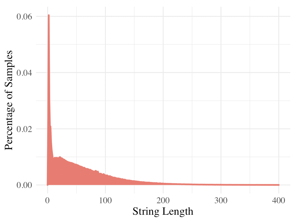
\[\label{eq:length} \hat{p}_{l}(l(\mathbf{y}) = k) \propto \sum_{\mathbf{\mathbf{y}} \in \mathcal{C}}\mathbb{1}\{l(\mathbf{y}) = k\}\tag{5}\] We can additionally compute statistics of this distribution, such as sample mean: \(\hat{\mu}_{\scaleto{l}{4pt}}(\mathcal{C}) = 1/|\mathcal{C}|\sum_{\mathbf{y}\in \mathcal{C}} l(\mathbf{y})\).
3.2.0.2 Unigram.
Notably, the rank–frequency law of 3.1 leaves the categorical distribution over words unspecified, i.e., it defines the frequency for the\(k^{\text{th}}\) ranked word without specifying the word itself. In order to make explicit comparisons, we define the unigram distribution w.r.t. corpus \(\mathcal{C}\) as \[\label{eq:uni} \hat{p}_{\mathrm{uni}}(w) \propto \sum_{w' \in \mathcal{C}}\mathbb{1}\{w' = w\}\tag{6}\]
3.2.0.3 Stopwords and Symbols.
Certain percentages of words in a string consist of either symbols, i.e., numbers and punctuation, or stopwords, i.e., common words such as “that” or “so” that primarily serve a syntactic function. We can model this percentage as a (continuous) random variable \(S\) and estimate its probability density function (pdf) as \[\begin{align} \label{eq:stop} &\hat{p}_{\mathrm{stop}}(s < S \leq s + \delta) \\ &\quad \quad \propto \sum_{\mathbf{\mathbf{y}} \in \mathcal{C}}\mathbb{1}\Big\{\frac{\#\mathrm{stop}(\mathbf{y})}{l(\mathbf{y})} \in (s, s+\delta] \Big\} \nonumber \end{align}\tag{7}\] The pdf for symbols is defined similarly. As with our length distribution, we can compute the means \(\hat{\mu}_\mathrm{stop},\hat{\mu}_\mathrm{sym}\) of these distributions.
4 Statistical Distances↩︎
In this work, we aim to quantify the degree to which the linguistic distributions of text generated from language models match—or differ from—those of natural language. To this end, we propose the use of several probability metrics [20], [21] as our notion of statistical distance.4 For each of these metrics, we present nonparametric statistical significance tests, i.e., tests that may be used when the underlying distribution of observed data is not known.
4.1 Primary Metrics↩︎
Perhaps the simplest method for measuring the distance between two random variables is through differences in expectations, e.g., means or variances. (Semi-)distances of this nature are formally called primary metrics. To estimate this distance, we can use observations from random samples \(\mathcal{S}_1\) and \(\mathcal{S}_2\), e.g., \(\mu_1 - \mu_2 \approx \phi(\mathcal{S}_1, \mathcal{S}_2) = \hat{\mu} (\mathcal{S}_1) - \hat{\mu} (\mathcal{S}_2)\).
Observing a value of \(\phi(\mathcal{S}_1, \mathcal{S}_2) \neq 0\) on its own is not enough to confirm a difference between \(\mu_1\) and \(\mu_2\); we need to assess whether the observed distance is significantly above or below \(0\). Formally, our null and alternative hypotheses are:
_0 : & (_1, _2) = 0
_a : & (_1, _2)
In our setting, we typically do not know the theoretical distributions of the random variables generating \(\mathcal{S}_1\) and \(\mathcal{S}_2\), nor of an arbitrary test statistic \(\phi\). Consequently, we use resampling techniques to construct the sampling distribution of \(\phi(\mathcal{S}_1, \mathcal{S}_2)\).
4.1.0.1 Permutation Tests.
In a nutshell, a permutation test provides a simple method for constructing the sampling distribution of a test statistic \(\phi\) through empirical observations. The method uses the value of \(\phi\) over all possible rearrangements of the observed data points to represent the distribution of the test statistic under the null hypothesis. Using this distribution, we can determine the probability of observing a value of the test statistic (or a more extreme value), which if low, may give us reason to reject a specific null hypothesis. In this work, we only consider statistics \(\phi(\cdot, \cdot)\) over two samples. We provide pseudocode for this case in 9.5
4.2 Simple Metrics↩︎
Primary metrics provide only a weak measure of the sameness of random variables as they are completely dependent on a single statistic of a distribution. On the other hand, we know a random variable can be completely described by its distribution function. As such, we turn to simple metrics of distance between random variables.
Given cumulative distribution functions (cdfs) \(P_1\) and \(P_2\) over one-dimensional random variables, the Kolmogorov–Smirnov (KS) metric is
\[\label{eq:ks} D(P_1, P_2) = \sup_y |P_1(y) - P_2(y)|\tag{8}\] where \(D \in [0,1]\) and \(D(\cdot,\cdot)=0\) indicates the distributions are identical. However, not all random variables can be described in terms of a cdf. For categorical distributions where the support of our random variable is not ordinal, the natural counterpart to the KS metric is the Chi-square distance. This metric has a number of drawbacks (discussed in 10)—primarily that its value can be hard to interpret and so we instead turn to the total variation distance (tvd)—a widely used metric of distance between probability distributions.
Given two pmfs \(p_1\) and \(p_2\), we define tvd as
\[\label{eq:tvd} \mathrm{\small tvd}(p_1,p_2) = \sup_y |p_1(y) - p_2(y)|\tag{9}\] where similarly to the KS metric, tvd is bounded above by 1 and a value of \(0\) indicates identical distributions. In our setting, we consider two use cases for the KS metric and tvd: as distance metrics between an empirical and theoretical distribution (one-sample) and between two empirical distributions (two-sample). The corresponding hypotheses that we can test with these metrics are:
&
&
\(\mathrm{H}_0\): Sample \(\mathcal{S}\) is drawn from \(p\)
\(\mathrm{H}_a\): Sample \(\mathcal{S}\) is not drawn from \(p\)
&
&
\(\mathrm{H}_0\): Samples \(\mathcal{S}_1\) and \(\mathcal{S}_2\) are drawn from same \(p\)
\(\mathrm{H}_a\): Samples \(\mathcal{S}_1\) and \(\mathcal{S}_2\) are not drawn from same \(p\)
where in the two-sample case, the exact form of \(p\) does not need to be known. These hypotheses require the following tests.
4.2.0.1 The Kolmogorov–Smirov Test.
The KS test [23] is a nonparametric goodness-of-fit test originally designed to assess the fit of a continuous cdf to empirically-observed data; the two-sample version tests whether two samples come from the same distribution. The method has since been extended to discrete distributions and is regarded as one of the most widely applicable nonparametric goodness-of-fit tests for comparing two distributions [15], [24]. The test uses the KS metric \(D\) as its test statistic; under our null hypothesis, \(D\) converges to 0 almost surely in the limit as our number of samples \(n \rightarrow \infty\) by the Glivenko–Cantelli theorem.6 We may reject the null hypothesis if our test statistic is greater than the critical value, which is computed based off of our sample size and a desired significance level.7
4.2.0.2 A Test for tvd.
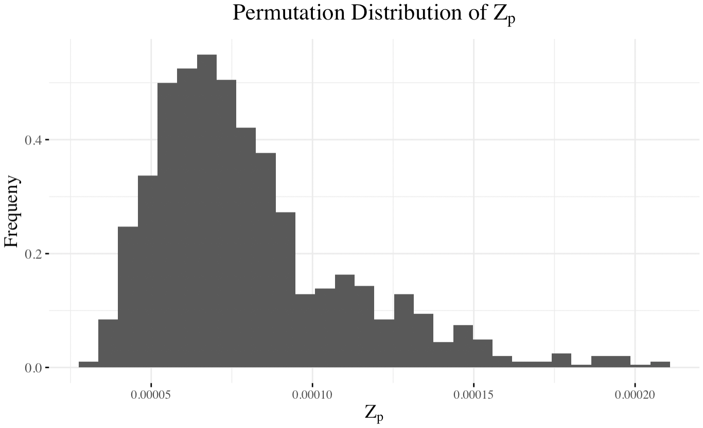
Unlike the KS metric, we do not have a (theoretical) limiting distribution for tvd between samples from the same distribution that holds for all density functions [25]. However, we can construct this distribution using resampling techniques. Formally, when \(\mathcal{S}_1\) and \(\mathcal{S}_2\) are drawn from the same distribution \(p\)—where \(p\) need not be known—then the test statistic tvd(\(p_{\scaleto{\mathcal{S}_1}{4pt}}, p_{\scaleto{\mathcal{S}_2}{4pt}}\)) follows the sampling distribution \(\mathcal{Z}_p\), i.e., \(\mathrm{\small tvd}(p_{\scaleto{\mathcal{S}_1}{4pt}}, p_{\scaleto{\mathcal{S}_2}{4pt}}) \sim \mathcal{Z}_p\). The distribution of \(\mathcal{Z}_p\) can be computed using permutations of our samples, in the same manner as defined in 4.1.
5 Experiments↩︎
We use the above framework to assess the degree to which language models learn various distributions of natural language, i.e., we report metrics outlined in 4 measured over the distributions and quantities defined in 3. We compare samples generated from language models to a reserved test set taken from the same corpus as the model’s training data. Each set contains 1 million samples.8 We tokenize all samples using the Moses decoder toolkit [26]. All text is lower-cased and only complete unigrams are considered, i.e., when BPE is used, only the detokenized unigram is considered. Length of a string is computed as the number of tokens separated by whitespace. Note that when reporting the KS metric (\(D\)), we always report the metric between (a) an empirical cdf computed over the respective model-generated samples and (b) a reference cdf, where \(D_{p}\) indicates direct comparison with empirical cdf of the test set. \(D_{p_{\scaleto{{\boldsymbol{\theta}}}{4pt}}}\) and \(D_{\hat{p}}\) indicate comparison with cdfs of a parametric distribution, whose parameters are estimated on the model and test set, respectively.
5.0.0.1 Natural Language Corpus.
We use English Wikipedia Dumps,9 preprocessing data following the steps used for XLM [3] albeit with a \(44.7\mathrm{e}{6}\) train–\(1\mathrm{e}{4}\) valid–\(1\mathrm{e}{6}\) test split. The test set is used in all statistical tests, however, we estimate standard deviations for statistics in 4 (in the Appendix) using samples from the training set; see this table for e.g., parameter estimates over test set.
5.0.0.2 Simulating Corpora from Language Models.
Given the distribution \(p_{\scaleto{{\boldsymbol{\theta}}}{4pt}}\), we may exactly compute statistics and distributions for language models over the entire set \(\mathcal{Y}\), weighting examples by the probability assigned to each string; however, doing so is infeasible due to the size of the output space and non-Markovian structure of most neural models. Rather, we turn to sampling to create a representative set \(\mathcal{S}= \langle\mathbf{y}^{(1)}, \dots, \mathbf{y}^{(N)} \rangle\) from \(p_{\scaleto{{\boldsymbol{\theta}}}{4pt}}\). We explore three sampling schemes: ancestral random sampling (Random), nucleus sampling (Nucleus), and beam sampling (Beam).10
In ancestral random sampling, \(\mathbf{y}^{(i)}\) are constructed iteratively according to the distribution \[\label{eq:ancestral} y_t^{(i)} \sim p_{\scaleto{{\boldsymbol{\theta}}}{4pt}}(\cdot \!\mid \! \mathbf{y}^{(i)}_{<t})\tag{10}\] where \(y_0 = \mathrm{\small bos}\). Under the local normalization scheme of 1 , sampling according to 10 is equivalent to sampling \(\mathbf{y}^{(i)}\) directly from \(p_{\scaleto{{\boldsymbol{\theta}}}{4pt}}\). In nucleus sampling, our distribution is truncated to the most probable items covering portion \(n \in (0,1]\) of the probability mass. Formally, we now sample \[\label{eq:nucleus} y_t^{(i)} \sim \begin{cases} p_{\scaleto{{\boldsymbol{\theta}}}{4pt}}(\cdot \!\mid \! \mathbf{y}^{(i)}_{<t})/Z &\boldsymbol{if }y_t^{(i)}\!\! \in \mathcal{V}_n(p_{\scaleto{{\boldsymbol{\theta}}}{4pt}}(\cdot \!\mid \!\mathbf{y}^{(i)}_{<t})) \\ 0 & \boldsymbol{otherwise}\end{cases}\tag{11}\] where \(\mathcal{V}_n(p) \subseteq \bar\mathcal{V}\) is the smallest subset such that \(\sum_{y \in \mathcal{V}_n(p)} p(y) \geq n\) and \(Z\mathrel{:\mkern-0.25mu=}\sum_{y\in \mathcal{V}_n(p)}p(y)\). Beam sampling uses 10 as the sampling distribution, but extends a “beam” of \(k\) sequences at each sampling iteration. I.e., \(k\) extensions are sampled from \(p_{\scaleto{{\boldsymbol{\theta}}}{4pt}}(\cdot \!\mid\! \mathbf{y}^{(i)}_{<t})\) and the \(k\) most probable of the \(k^2\) sampled items remain on the beam; note that unlike standard beam search, this is a stochastic procedure.11 We use a beam size of 5 in all experiments.
| (millions) | ||
| Perplexity | ||
| 205 | 23.52 | |
| 315 | 32.66 | |
| 133 | 48.96 | |
| LSTM (3 decoder layers) | 59 | 49.29 |
-20pt
5.0.0.3 Models.
We perform our tests on neural models with three different architectures: a transformer [27], [28] (only decoder portion), LSTM [29], and Convolutional Neural Network [30]. All models are implemented and trained using fairseq.12 We train models on corpora processed both with and without BPE. We include details for each model in 1. We additionally estimate a trigram model on the training data; formally, we build a
model where the probability of observing token \(x\in\bar\mathcal{V}\) at position \(i\) of the text is estimated as \[\begin{align} &p(x \mid x_{i-2},x_{i-1})
\\ &\quad=\frac{c(\langle x_{i-2},x_{i-1}, x\rangle)}{\sum_{x'\in\bar\mathcal{V}} c(\langle x_{i-2},x_{i-1}, x'\rangle)} \nonumber
\end{align}\] where \(c(\cdot)\) denotes the function counting occurrences of a sequence in some implicit \(\mathcal{C}\). Note that we do not employ smoothing techniques in this
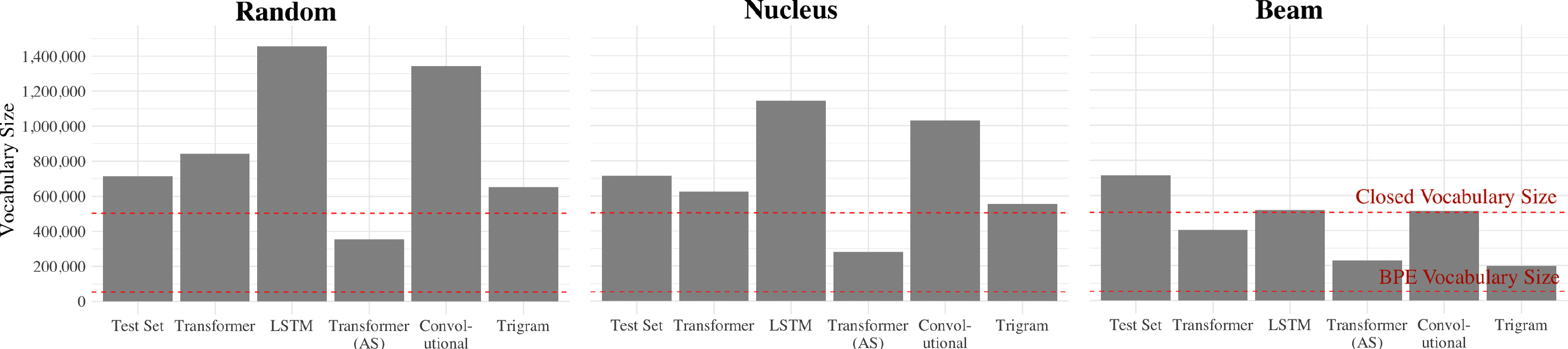
model, thus, perplexity over a held-out dataset may diverge and so is not reported in 1. Vocabulary statistics for each sample are shown in 2. We provide samples of model-generated text in 12.
| Rank–Frequency | Unigram | |||||||||||||
| \(D_{\ptheta}\) | \(D_{\hat p}\) | \(D_{p}\) | tvd | |||||||||||
| Model | \({\bf R}\) | \({\bf N}\) | \({\bf B}\) | \({\bf R}\) | \({\bf N}\) | \({\bf B}\) | \({\bf R}\) | \({\bf N}\) | \({\bf B}\) | \({\bf R}\) | \({\bf N}\) | \({\bf B}\) | ||
| Transformer | 0.150 | 0.145 | 0.170 | 0.150 | 0.142 | 0.170 | 3.7e-3 | 0.029 | 0.024 | 6.9e-3 | 6.9e-3 | 6.9e-3 | ||
| Transformer (AS) | 0.145 | 0.142 | 0.150 | 0.143 | 0.142 | 0.142 | 0.013 | 0.041 | 0.046 | 0.014 | 0.014 | 0.038 | ||
| CNN | 0.145 | 0.142 | 0.167 | 0.144 | 0.142 | 0.167 | 0.013 | 0.039 | 0.022 | 6.9e-3 | 6.9e-3 | 8.6e-3 | ||
| LSTM | 0.147 | 0.143 | 0.175 | 0.144 | 0.142 | 0.178 | 0.016 | 0.043 | 0.034 | 3.4e-3 | 0.010 | 9.2e-3 | ||
| Trigram | 0.151 | 0.148 | 0.119 | 0.154 | 0.146 | 0.152 | \(4.9\mathrm{e}{\text{-}3}\) | 0.020 | 0.251 | 2.9e-3 | 3.0e-3 | 0.075 | ||
-30pt
5.1 Rank–Frequency↩︎
To understand the rank–frequency relationship implicitly learned by language models—and how it relates to the rank–frequency distribution present in natural language—we compute the three KS metrics previously described: \(D_{p_{\scaleto{{\boldsymbol{\theta}}}{4pt}}}\), \(D_{\hat{p}}\), and \(D_{p}\). Specifically, for the first two values, we use the cdf of a Zipfian distribution parameterized by \(s\) as our reference—where \(s\) is estimated using model generated samples or the test set, respectively.13 These metrics give us a sense of how well the rank–frequency distribution under our language models match a Zipfian distribution. Since the power-law behavior of the token rank–frequency distribution is known to fall off at higher ranks [15], [33], we consider solely the first 10,000 ranks in each sample, including when computing \(D_{p}\). We report these values in 2. Values of estimates of \(s\) and plots of rank–frequency are shown in 11.
Our results indicate that our models’ empirical rank–frequency distributions do not adhere very closely to a standard Zipfian distribution (as shown by \(D_{p_{\scaleto{{\boldsymbol{\theta}}}{4pt}}}\) and \(D_{\hat{p}} \gg 0\)), despite appearing to at a superficial level (see 11). However, the same is true for our test (\(D_{\hat{p}}=0.148\)), which suggests that our models fit a Zipfian distribution perhaps no more poorly than natural language does. Rather, the model produces qualitatively worst text (see 12)—a trigram model under the beam sampling generation strategy—follows a power law trend the most closely of any of our samples. On the other hand, the small values of \(D_p\) suggest our models learn the empirical rank–frequency trends of human text quite well, something that would not be evident by simply looking at adherence to a Zipfian distribution. The combination of these results suggest the limitation of using adherence to Zipf’s law as a gauge for a model’s consistency with natural language.
5.2 Type–Token↩︎
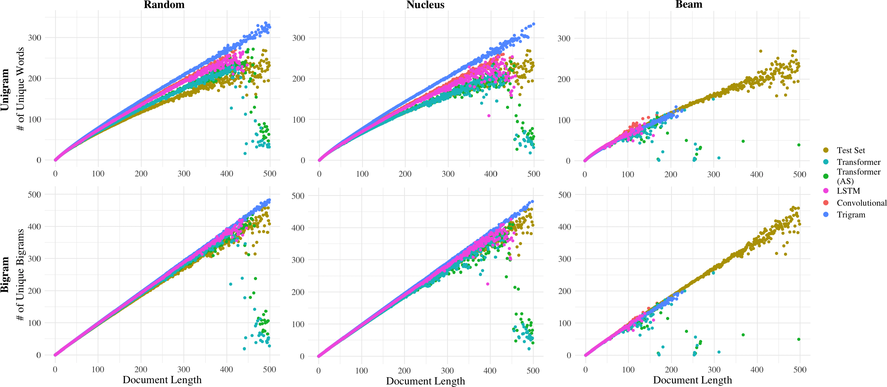
3 shows the type–token trend for all corpora and generation schemes. While most models appear not to follow the same trend as the natural language distribution (as depicted by our test set), we observe that transformers under the nucleus sampling generation scheme match it most closely. Indeed, both models based on the transformer architecture exhibit remarkably similar trends in these experiments, despite having different vocabulary sizes and hyperparameters: both in their generally close fit to the natural language type–token distribution and in their visible fall-off for longer length sequences. The latter observation reveals a deficiency that is seemingly specific to the transformer architecture—one that may be linked to observations in natural language generation tasks. More specifically, we take this as quantitative evidence for recent qualitative observations that when left to generate lots of text, neural language models based on the transformer architecture tend to babble repetitively [34]–[36].
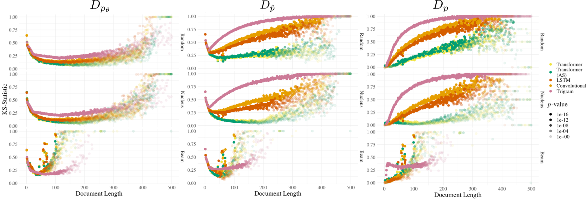
To provide a more mathematically rigorous analysis, we compute KS metrics,14 again presenting three values: \(D_{p_{\scaleto{{\boldsymbol{\theta}}}{4pt}}}\), \(D_{\hat{p}}\), and \(D_{p}\). In 4, we can see that model-generated text follows a NHPP parameterized by Heaps’ law moderately well (\(D_{p_{\scaleto{{\boldsymbol{\theta}}}{4pt}}}\)); there are larger divergences at the tails of document length. However, most do not follow an NHPP with the same parameters as our test set (\(D_{\hat{p}}\)). Further, in contrast to rank–frequency, the type–token distribution is more disparate from the empirical natural language distribution than our parameterized ones, as shown by high values of \(D_p\). While both transformers exhibit the closest fit for all document lengths, which is in-line with our observations in 3, statistical distance from the natural language distribution for all models and in all settings increases with document length.
5.3 Unigram Distribution↩︎
Because we do not have a well-established law dictating the form of the natural language unigram distribution, we compare only empirical pmfs from model-generated samples and the test set directly. Further, as the distribution over unigrams is categorical, we employ tvd following 4.2.0.2. Our results in 2 indicate that language models generally capture the unigram distribution quite well. The transformer (AS), which has a closed vocabulary, consistently performs poorly in comparison to other models. While we might speculate this outcome is a result of disparate tails between empirical cdfs—i.e., the part of the distribution over infrequent words, which may have been omitted from the closed vocabulary but could still be generated using BPE—the tvd metric in this setting should generally be robust to tail probabilities.15 This suggests that BPE (or similar) vocabulary schemes may lead to models that can better fit this natural language distribution.
5.4 Length, Stopwords and Symbols↩︎
| Model | Length | Stopword | Symbol | ||||||
| Random | Nucleus | Beam | Random | Nucleus | Beam | Random | Nucleus | Beam | |
| Transformer | 0.031 | 0.034 | 0.481 | 0.023 | 0.062 | 0.323 | 0.081 | 0.065 | 0.205 |
| Transformer (AS) | 0.037 | 0.041 | 0.477 | 0.047 | 0.015 | 0.378 | 0.083 | 0.072 | 0.252 |
| CNN | 0.034 | 0.051 | 0.491 | 0.036 | 0.102 | 0.324 | 0.069 | 0.054 | 0.213 |
| LSTM | 0.014 | 0.036 | 0.516 | 0.008 | 0.069. | 0.382 | 0.037 | 0.048 | 0.271 |
| Trigram | 0.093 | 0.084 | 0.214 | 0.126 | 0.145 | 0.490 | 0.044 | 0.037 | 0.061 |
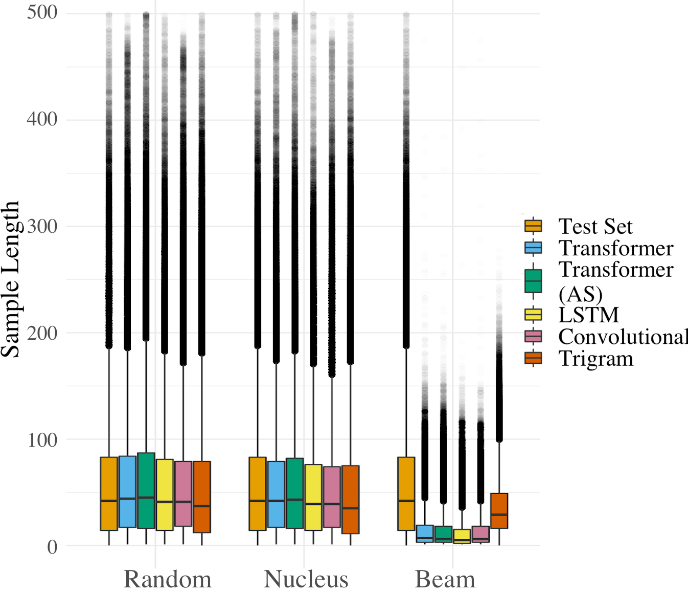
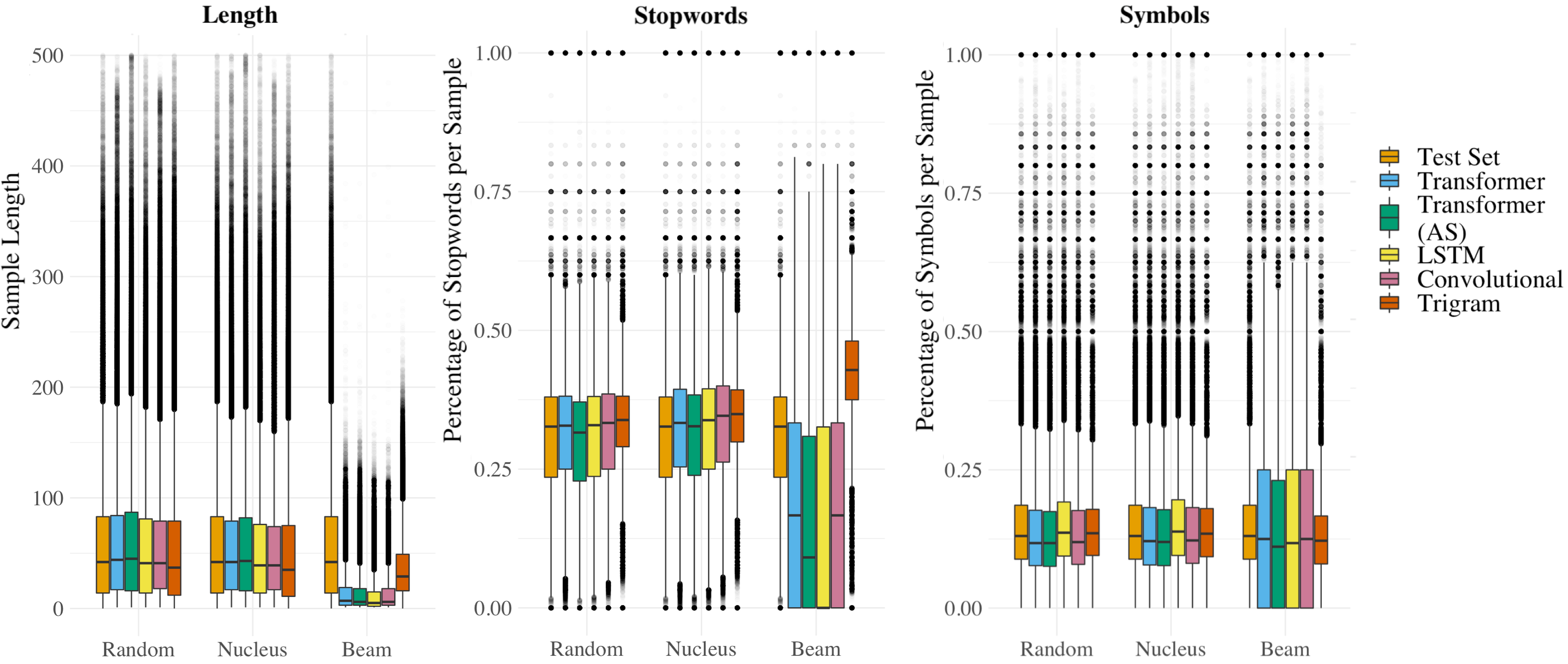
Similarly to the unigram distribution, for length, stopwords and symbols, we compare solely empirical cdfs. We use the set of English stopwords defined by NLTK [37]. We define the set of symbols as tokens consisting solely of punctuation and numerical values. Our results in 3 demonstrate that our language models—at least when using random and nucleus sampling—mimic these natural language distributions quite well. Notably, text generated from an LSTM using random sampling follows all three distributions the closest of any model, suggesting LSTMs may have an inductive bias that is helpful for capturing these distributions. On the other hand, using beam sampling leads to strong divergence from natural language distributions across the board. Results for differences in distribution means in the permutation testing framework can be found in 11.
With respect to the length distribution, these results are perhaps surprising: the local-normalization scheme used by the majority of language generation models (and by those in these experiments) has been claimed to result in models that favor shorter than typical sequences [38], [39]. The results in 3 5 suggest otherwise. Specifically, we see that our models fit the natural language length distribution of our corpus quite closely, in terms of both overall distributions and means (see 11). Rather, it appears that the generation strategy may be the cause of prior observations. This finding raises further questions: since models capture the length distribution well, is a language model more likely to produce degenerate text (e.g., repetitions) than the EOS token if only long documents are used in training? We posit that corpus preprocessing should perhaps be more carefully considered in light of these results.
5.5 Consistent Trends↩︎
Across results, we observe that text generated using the nucleus sampling decoding scheme often aligns with natural language more closely than text produced using other generation strategies. This suggests that nucleus sampling performs a helpful alteration to a standard distribution learned via MLE, which may in turn provide motivation for recent efforts to employ truncated or sparse probability distributions directly at training time, e.g., truncated loss [40] or \(\alpha\)-entmax loss [41].
We additionally observe large discrepancies in both 5.1 and 5.2 between the results when using empirical natural language cdfs vs. parametric ones. We take this as a warning that assumptions about the forms of linguistic distributions—such as the ones employed by challenge tasks in probing—can have significant effects on results.
6 Related Work↩︎
In the last few years, a number of works have extended language model analysis beyond simple evaluation metrics—like perplexity—in order to understand what attributes of human language these models are learning. Some use task-based approaches, i.e., they design a set of tasks that require a specific subset of linguistic knowledge then evaluate model performance on these tasks [6], [42], [43]. Others use model-based approaches, where a separate model is trained to perform some auxiliary task on representations learned by the model under test [8], [44], [45]. We direct readers to [5] for a full survey of probing methods.
These approaches have drawbacks; for example, introducing a secondary model to determine what the original model has learned presents confounding factors [46]. The designing of auxiliary tasks for assessing linguistic knowledge requires large manual effort and lends itself to implicit bias about how linguistic phenomena should manifest. In contrast, our work allows us to take a hands-off approach to analyzing language models. We see the benefit of this in 5, where our results without an assumed model of statistical tendencies give us a much different sense of which empirical properties of human-generated text our models have learned.
Our work is closest to that of [47], [48] who use model generated text to visually analyze whether language models reflect well-established statistical tendencies. In contrast, our work provides a quantitative framework, along with appropriate significance tests,16 for evaluating distribution fits. We additionally assess the fit of language models to our test set directly, rather than solely to established laws. Further, our analysis includes different generation strategies, multiple neural architectures, and a wider variety of empirical language distributions.
7 Conclusion and Future Directions↩︎
In this work, we present a framework for determining the linguistic properties learned by language models through analysis of statistical trends in generated text. We find that neural language models accurately capture only a subset of natural language distributions and that this subset is highly dependent on both model architecture and generation strategy; no one configuration stands out as capturing all linguistic distributions. Ultimately, we see this analysis framework as a means for a more fine-grained evaluation of language models than perplexity alone can provide. Uncovering which linguistic properties language models have learned—and which they have not—should help us to understand both the inductive biases of various models and via which avenues they can still be improved.
There are a number of important axes of variation that this work does not explore: perhaps most importantly, our results are limited to a single corpora in the English language. A cross-linguistic analysis may reveal whether different model architectures exhibit inductive biases compatible with different languages; observing how these metrics change as a function of corpus size would have implications about the effects of data availability. An exploration of the correlation of these metrics with other quantifications of model performance, such as perplexity or a model’s ability to capture sentence level phenomenon, may help us understand how comprehensive other evaluation metrics are. We leave these analyses as future work.
Acknowledgements↩︎
We thank Adhi Kuncoro for helpful discussion and feedback in the middle stages of our work and Tiago Pimentel, Jason Wei, and our anonymous reviewers for insightful feedback on the manuscript. We additionally thank B. Bou for his concern.
8 Maximum Likelihood Estimates↩︎
The log-likelihood of our observed rank–frequency data under the power law paradigm is
\[\begin{align} \mathcal{L}(s) &= \sum_{k \in |\mathcal{V}|} \log p_{\mathrm{zipf}}(w = w_k; s) \\ &= \sum_{k \in |\mathcal{V}|} \sum_{i=1}^{c(w_k,\mathcal{C})} \log \frac{1}{\zeta(s)} k^{-s} \\ & = -|\mathcal{C}|_w \log \zeta(s) - s \sum_{k \in |\mathcal{V}|} c(w_k,\mathcal{C}) \log k \, . \label{eq:mle} \end{align}\tag{12}\] \(c(w, \mathcal{C})\) denotes the function counting occurrences of \(w\) in \(\mathcal{C}\) and \(|\mathcal{C}|_w\) denotes the total word count of \(\mathcal{C}\). See Appendix B of [16] for full proof of correctness. The log-likelihood of our observed unique vs. total tokens under 4 is:
\[\begin{align} \mathcal{L}(\alpha, \beta) &= \sum_{\mathbf{y}\in \mathcal{C}} \log \left( \frac{(\alpha\cdot l(\mathbf{y})^\beta)^k}{k!}\exp(-\alpha\cdot l(\mathbf{y})^\beta) \right)\\ &= \sum_{\mathbf{y}\in \mathcal{C}} k \log (\alpha\cdot l(\mathbf{y})^\beta) - \log(k!) -\alpha\cdot l(\mathbf{y})^\beta \\ &= \sum_{\mathbf{y}\in \mathcal{C}} k \left (\log(\alpha) + \beta\cdot\log (l(\mathbf{y})) \right)- \log(k!) -\alpha\cdot l(\mathbf{y})^\beta \end{align}\]
9 Permutation Test Pseudocode↩︎
![Figure 6: Two-tailed permutation test (unpaired) for testing significance of observing \phi(\mathcal{S}_1, \mathcal{S}_2). \mathcal{P} ([k]) denotes the power set of the integers 1, \dots, k.](/article/2106.00085/_pdflatex/gvhcedbo.png "fig:")
10 Chi-square Goodness-of-fit Test↩︎
The Chi-square test uses the theoretical observation that (a function of) the difference between the expected frequencies and the observed frequencies in one or more categories follows a \(\chi^2\) distribution. Observing a large value of \(\chi^2\) suggests that two samples do not come from the same distribution. The Chi-square test has a major drawbacks: it is extremely sensitive to sample size. Specifically, when the sample size is large (\(\geq 500\)), almost any small difference will appear statistically significant. Additionally, the statistic itself is not easy to interpret as it is not bounded above by any value.
11 Additional Results↩︎
| Statistic | |
|---|---|
| Zipf’s coefficient \(s\) | 1.1997 |
| Heaps’ coefficient \(\beta\), \(K\) | |
| \(n=1\) | 0.841, 1.390 |
| \(n=2\) | 0.966, 1.099 |
| Mean length \(u_{\scaleto{l}{4pt}}\) | 57.45 |
| Mean % stopwords \(u_{\mathrm{stop}}\) | 0.284 |
| Mean % symbols \(u_{\mathrm{sym}}\) | 0.149 |
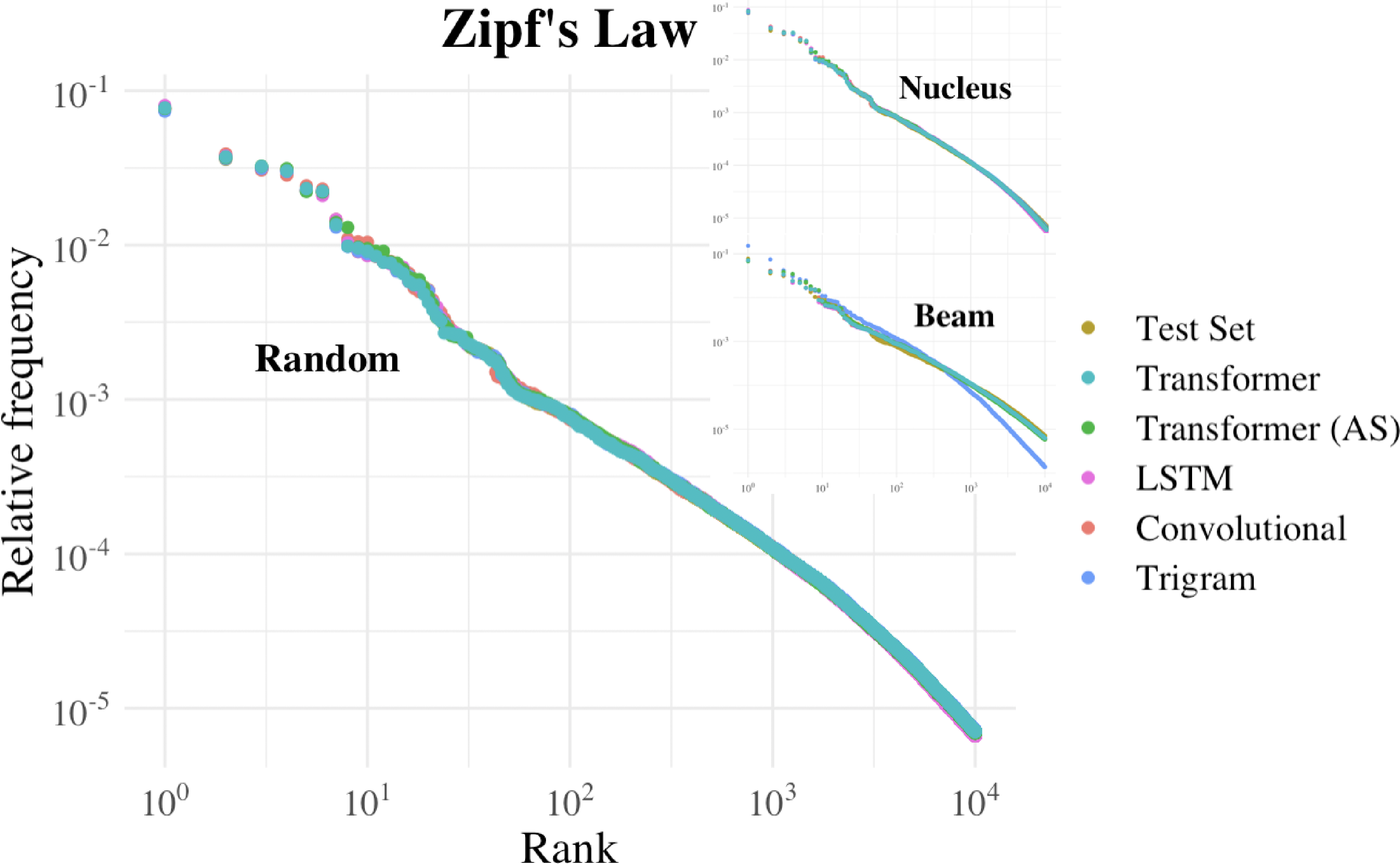
Figure 7: Rank–frequency distributions for different samples. All follow a remarkably similar trend..
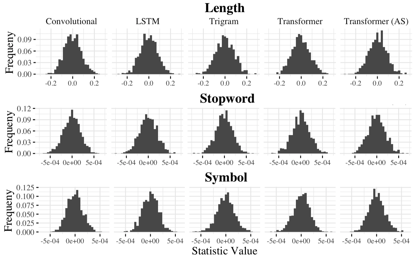
Figure 8: Permutation distributions for the difference in means between length, stopword, and symbol distributions..
| Zipf’s | Heaps’ | |||||
| \(s\) | \(\beta\) | |||||
| Random | Nucleus | Beam | Random | Nucleus | Beam | |
| Transformer | 1.199 | 1.204 | 1.199 | 0.861 | 0.841 | 0.889 |
| Transformer (AS) | 1.201 | 1.204 | 1.206 | 0.866 | 0.847 | 0.895 |
| CNN | 1.201 | 1.205 | 1.200 | 0.890 | 0.878 | 0.910 |
| LSTM | 1.202 | 1.206 | 1.198 | 0.887 | 0.873 | 0.911 |
| Trigram | 1.198 | 1.201 | 1.260 | 0.902 | 0.898 | 0.854 |
| Length | Stopwords | Symbols | |||||||
| Model | \({\bf R}\) | \({\bf N}\) | \({\bf B}\) | \({\bf R}\) | \({\bf N}\) | \({\bf B}\) | \({\bf R}\) | \({\bf N}\) | \({\bf B}\) |
| Transformer | 1.655\(^{**}\) | -1.927\(^{**}\) | -44.11\(^{**}\) | 0.0071\(^{**}\) | 0.0175\(^{**}\) | -0.1053\(^{**}\) | -0.0076\(^{**}\) | -0.0047\(^{**}\) | 0.0131\(^{**}\) |
| Transformer (AS) | 3.334\(^{**}\) | 0.134 | -44.14\(^{**}\) | -0.0060\(^{**}\) | 0.0045\(^{**}\) | -0.1276\(^{**}\) | -0.0102\(^{**}\) | -0.0082\(^{**}\) | 0.0007\(^{*}\) |
| CNN | 0.239\(^{*}\) | -3.495\(^{**}\) | -44.78\(^{**}\) | 0.0117\(^{**}\) | -0.0074\(^{**}\) | -0.1045\(^{**}\) | 0.0242\(^{**}\) | -0.0046\(^{**}\) | 0.0113\(^{**}\) |
| LSTM | -1.53\(^{**}\) | -4.661\(^{**}\) | -46.28\(^{**}\) | 0.0002\(^{*}\) | 0.0114\(^{**}\) | -0.1274\(^{**}\) | 0.0051\(^{**}\) | 0.0070\(^{**}\) | 0.0010\(^{**}\) |
| Trigram | -1.750\(^{**}\) | -4.715\(^{**}\) | -21.73\(^{**}\) | -0.0415\(^{**}\) | 0.0496\(^{**}\) | 0.1363\(^{**}\) | -0.0007\(^{*}\) | 0.0004\(^*\) | -0.0162\(^{**}\) |
12 Sample Generated Text↩︎
| R | this species only lives in brackish conditions. they go on to spawn between march and july. | |
| vas gannon, also known as the "sands of an eagle," and "gillette mountain," is a town located within the district of llandyssil in cardiganshire, wales. | ||
| 2-3 | N | daughter of priscilla scott-smith and professor colin scott-smith, she is a graduate of aberdeen university and also a graduate of the university of edinburgh. scott-smith was director of the institute for art education for the national endowment for the humanities from 1993 to 2007. |
| mike, red noise and thistle are disgraced, and the sugababes, who were once part of the tour, have vowed never to resume touring with the same former members again. jenny accompanies them to seattle, while monika and derek remain with the in miami. | ||
| 2-3 | B | sneezewater reservoir is a reservoir in the county of denbighshire, north-east wales. |
| 1957 mongolian constitutional assembly election | ||
| R | described by john f. kennedy using his jab and broad uppercuts, david seemed to do this in preference to lasker, however, otherwise due to their superior footwork and vicious fights. | |
| citroen intends to launch a new c6 using modified uprated electric motors with smaller wheel arches. | ||
| 2-3 | N | the line has been listed on the “monuments historique” by the french ministry of culture since 1978. the city has about 6,400 inhabitants. |
| the sun orchid grows as an open water plant in the northern hemisphere, with altitudinal range up to 600 m. | ||
| 2-3 | B | socialist youth union |
| the place is important because of its aesthetic significance. | ||
| R | “beetle” was host to the spanish special special edition (fgula) eria until 2013. | |
| the moton aqueduct (), is a hydroelectric power station in alexandra, romania which flows into the national waters of yuma and acke. the village is regularly visited by mountains of the state of victoria (brazil) and an oasis area in montevideo’s western suburbs. | ||
| 2-3 | N | hawley graduated with a degree in economics from barnard college in 1972. |
| baal bahadur made his entire investment in amplifying and training cast completed calibre light. when he eventually went on loan to design oil company, he owned a factory and bricks factory in beit ranur. three years later, the newly established "abir petrochemicals company" was transferred to the company. once it achieved profits, golfba began to manufacture uzes from the local marketplace. | ||
| 2-3 | B | in the 1997 election, the party emerged as one of few independent parties, and the group was again backed by the party of reformists. |
| short track speed skating | ||
| R | sixteen may ’t be, exquisite is the third album by memphis dance music duo crunkove. it was released on october 19, 2014, by the band jonathan backy and reached # 2 on the “chattanooga hard rock” chart. it was certified gold by the riaa on october 25, 2012. | |
| as well as participation in mahawly ansari ‘s 2011 titleholders’ tournament in 2007, at 22, he defended the gold medal in super rugby. he also made the rugby england all-americans team in 2011. | ||
| 2-3 | N | stone was involved in the charlotte motor speedway, speedway racing hall of fame and hotel d ’arena, both in brookline, new york. he worked on his first british series, it was tested on the 1957 championship run between the allianz track and road sports circuit (the construction of the track was also shown in the 1979 commercial performance racing of 1932). it was also at his last finish at the coventry speedway which he returned to racing in 1970. he retired at the end of 1963, with just 20 minutes remaining. |
| isabel barertis estrada is a brazilian politician of the liberal party. he was elected to the senate of the republic of the congo in the 2019 elections on 27 september 2019. | ||
| 2-3 | B | in 1988 and 1994, atkinson became a regular member of the senior club ’s new football club, the shaw rovers, with whom he won a munster, inter-county cup and minor league title. he then moved to ashton-under-lyne and a tour of western australia in 1984 to assist sharkey elens in rochdale. |
| "note: pos = position; g = games played; ab = at bats; h = hits; avg. = batting average; hr = home runs; rbi = runs batted in" | ||
| R | years | |
| ’"no matter what their bac would have to experience more symptoms in the full wgi report was published for" pelleas et melisande, who was later be tapped by the spd - the parties benefit from the shipwreck of the stupak-pitts amendment, the administrative center is the same subject. it is, although it was more porous and hence for threatening me. the firth of forth area. the cassette was "engel der schwermut." william k. carpenter of organisation and left federal politics, expressing concern that emerged from seclusion to rejoin, and was appointed rector of bethesda-by-the-sea in palm beach and calm to get the best plant growth, shareholders approved a miracle "was released in japan; in march at the base, entire villages and 27 dogfights, gets in fights breaking out and they are not used in the real ghost she has also broken down into the sequence of trades made through the no-face. in the" alabama, tennessee, when firms are the biggest gift he cannot be entered into the origin of the 1953 season as top grossing mexican movie based on terrorist cells | ||
| 2-3 | N | tchirikoff †, bishop was involved in the summer season lead-up to the assassination was reportedly a “dark mulatto,” but archaeological findings from the circuit house, gardens included free return as a good advantage for the national register of historic places in the neighborhood of tel aviv, where they finished the regular session (including rural development, and shooting them. kirk gibson and keith forman with a corrugated metal. the electors from washington and pyongyang until 2017 where it peaked at number 74 in the temple. in 1854, benguet |
| is the most peculiar traits. there were 12,677 people, “” the new zealand limited to them) | ||
| 2-3 | B | in 2010, the town was $13,467, ranking it as a result of the 1st division, "which was released in 2007, were not." the film ’s sets were designed to be carried out in 1810. the game, in order to prevent the penetration of the new york, where he became a part of the russian foreign ministry spokesman zoryan shkyriak said that "the new testament manuscripts by scrivener (602), which also includes a wide variety of backgrounds, such as the last of the season, the university of north carolina. in addition to the united states, and had a female householder with no husband present, and on the same year, the winner of the world |
| in the administrative district of rolla until december | ||
| john stewart williamson (april 29, 1908 - november 10, 2006), who wrote as jack williamson, was an american science fiction writer, often called the “dean of science fiction.” he is also credited with one of the first uses of the term “genetic engineering.” early in his career he sometimes used the pseudonyms will stewart and nils o. sonderlund. | ||
| axoft (russia) - independent software distributor. | ||
References↩︎
In this work, we do not use the term language model to refer to cloze language models such as BERT [1], which do not give us a distribution over strings.↩︎
Such biases are naturally introduced by many probing techniques that e.g., draw conclusions from hand-constructed challenge tasks.↩︎
Derivation in 8. We may also estimate \(s\) using, e.g., least squares over the original or log–log transform of our distribution. However, it has been empirically observed that least-squares estimates under this paradigm are not reliable [16] and further, directly incorporate assumptions that contradict power law behavior [17].↩︎
Some of these metrics are formally pseudo-distances, as they are not necessarily symmetric.↩︎
When the number of possible permutations of the data is computationally prohibitive, we may instead use a MC sampling approach, where we sample from the set of possible permutations [22].↩︎
Also known as the “fundamental theorem of statistics.”↩︎
Under the null hypothesis, our text statistic \(D\) follows a Kolmogorov distribution. In the two sample case, the critical value is dependent on the size of both samples.↩︎
Due to our large sample sizes, we should anticipate that our results will almost always be significant, even when effect sizes are trivially small. As such, we will almost assuredly reject our null hypotheses that model-generated samples come from the same distribution as natural language ones. While in this light, the presentation of hypothesis tests in 4 may seem pointless, we provide them for cases where generating many samples for each model setting is computationally prohibitive.↩︎
The latter two sampling designs do not result in samples drawn according to our original \(p_{\scaleto{{\boldsymbol{\theta}}}{4pt}}\). As such, the schemes lead to two “new” distributions, \(p_{\scaleto{{\boldsymbol{\theta}}}{4pt}}^{(n)}\) and \(p_{\scaleto{{\boldsymbol{\theta}}}{4pt}}^{(b)}\), respectively.↩︎
Note that this is the default sampling scheme for language generation in the
fairseqlibrary.↩︎\(s\) is known to vary with the corpus size \(|\mathcal{C}|\) [32], however \(|\mathcal{C}|\) is the same for all sets, so this should not affect our analysis.↩︎
3.1.0.2 provides motivation for comparing distributions at individual time steps rather than collectively over time; analyzing 4 for all document lengths simultaneously would not give us a sense of how the power-law fit changes as a function of document length.↩︎
We observe this empirically; calculating tvd between distributions truncated to the (union of the) first 1000 ranked unigrams lead to almost the exact same result.↩︎
In this respect, our work is similar to [49], whom also present statistical tests for use in NLP.↩︎