On the Effectiveness of Dataset Embeddings in Mono-lingual, Multi-lingual and Zero-shot Conditions
March 01, 2021
Abstract
Recent complementary strands of research have shown that leveraging information on the data source through encoding their properties into embeddings can lead to performance increase when training a single model on heterogeneous data sources. However, it remains unclear in which situations these dataset embeddings are most effective, because they are used in a large variety of settings, languages and tasks. Furthermore, it is usually assumed that gold information on the data source is available, and that the test data is from a distribution seen during training. In this work, we compare the effect of dataset embeddings in mono-lingual settings, multi-lingual settings, and with predicted data source label in a zero-shot setting. We evaluate on three morphosyntactic tasks:morphological tagging, lemmatization, and dependency parsing, and use 104 datasets, 66 languages, and two different dataset grouping strategies. Performance increases are highest when the datasets are of the same language, and we know from which distribution the test-instance is drawn. In contrast, for setups where the data is from an unseen distribution, performance increase vanishes.1
1 Introduction↩︎
The performance of natural language processing systems is dependent on the amount of training data, which is often scarce. To complement existing training data, supplementary data sources can be used. Especially data annotated for the same task from other sources can be beneficial to exploit. However, because of heterogeneity in language or domain this might lead to sub-optimal performance. In early work on combining training sources, data was selected at training time [1], [2] for a given test set. A more nuanced way to exploit heterogeneous data is to encode properties of the language as features [3].
Recently, showed that encoding the language of an instance as an embedding in a neural model is beneficial for multi-lingual learning.2 Follow-up work found that multiple datasets within the same language can also be combined by encoding their origin [5], [6], thereby implicitly learning useful commonalities, while still encoding dataset-specific knowledge. These dataset embeddings are employed in groups of datasets which usually range in size from 2 to 10 datasets. However, it remains unclear in which situations these dataset embeddings thrive best.
Furthermore, two often overseen issues with dataset embeddings are that they are commonly learned from the gold data-source labels attached to each training and test instance and it is assumed that the test data is from a distribution which is seen during training. In many real world situations these assumptions are clearly violated. A common strategy when the test data is drawn from a different distribution as the training datasets (zero-shot), is to use a manually assigned proxy treebank [7]–[9]. Recent work showed that for unseen datasets in mono-lingual setups [10], interpolated dataset embeddings can be used to improve performance for zero-shot settings. We use automatically predicted proxy data sources instead, and focus on mono-linugal as well as cross-lingual setups.
In this paper, we provide an extensive evaluation of the usefulness of dataset embeddings in existing setups and beyond. More concretely, we ask: 1) What are good indicators to predict the usefulness of dataset embeddings? 2) Can we effectively use dataset embeddings in the absence of gold data-source information?
2 Dataset Embeddings↩︎
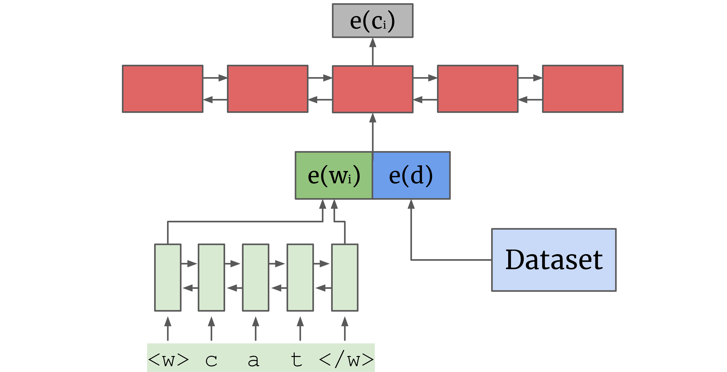
Dataset embeddings enable conditioning of inputs on some property of the data when training on multiple sources. They are vector representations learned during model training, with the aim to capture distinctive properties of the sources into a continuous vector, without losing their heterogeneous characteristics. Given \(D\) data sources, technically, we learn a vector representation \(e(d)\) for each data source \(d \in D\) while training a single model from a group of sources. Every input instance marked with its dataset source \(d\). For each word \(w_i\) with \(i=0, ..., n\), the word embedding \(e(w_i)\) is concatenated with the dataset embedding \(e(d)\), and both are updated during training. Figure 1 shows the overall architecture of the model which employs a contextual encoder that uses the resulting embedding as input and outputs \(e(c_i)\) to be used for prediction.
2.1 Experimental Setup↩︎
In this work, we copy the exact setups from the UUParser 2.3 [7] and the Multi-Team tagger [6] because they were high ranking systems in two recent shared tasks [11], [12] and they both showed large gains by using dataset embeddings. The UUParser is an Arc-Hybrid [13] BiLSTM [14] dependency parser, which exploits a dynamic oracle [15] and supports non-projective parsing through the use of a swap action [16]. The Multi-Team tagger performs morphological tagging [17] and lemmatization jointly; to this end, they use a shared BiLSTM encoder and feed the output of the tagging as input for the lemmatization, which is predicted as a sequence of characters. For efficiency reasons and simplicity, we disabled the use of external embeddings3 as well as POS embeddings for the UUParser.
It should be noted that besides the differences in the models and tasks, the setups also differ among several aspects; the version of UD data (2.3, 2.2) [18], type of dataset splitting used (Multi-Team always has train-dev-test), and most interestingly, the dataset grouping strategies. manually designed dataset groups based on typological information, language-relatedness and empirical evidence; instead propose pairs:every dataset is matched with one other dataset based on word overlap. For both of the models, we copy the exact language grouping as in the original papers4. For comparison of different grouping strategies, we refer to .
| Morphological Tagging (F1) | Lemmatization (Accuracy) | Dependency Parsing (LAS) | ||||||||||||
| Filtering | #src | base | concat | gold | pred | base | concat | gold | pred | #src | base | concat | gold | pred |
| All | 104 | 92.04 | 91.43 | 92.75 | 91.85 | 91.10 | 91.02 | 92.55 | 91.41 | 58 | 72.92 | 74.07 | 75.53 | 74.52 |
| Single-lang | 59 | 94.14 | 93.94 | 95.84 | 94.13 | 93.66 | 93.83 | 95.73 | 93.84 | 10 | 80.48 | 79.84 | 82.74 | 80.29 |
| Multi-lang | 45 | 89.30 | 88.14 | 88.69 | 88.88 | 87.75 | 87.33 | 88.38 | 88.22 | 48 | 71.35 | 72.87 | 74.03 | 73.32 |
3.5pt
2.2 Data Source Prediction↩︎
In this work, we predict data source on the sentence level, because it matches the language switches at test-time and it improves the accuracy of the classification.5 We use a linear support vector classifier based on word and character n-grams (without tokenization). We use this approach here because of simplicity, efficiency and they have shown to reach competitive performance for text classification tasks [19]–[22]. We performed a grid search with \(n \in [1-7]\) and all sequential combinations (1-2, 1-3, etc.) for \(n\)-grams. For this hyper-parameter tuning, we used the eight datasets from , and found the most robust parameters to be 1-2 for words and 1-5 for characters. The obtained macro average F1 on all data pairs from is 95.42, and on all data groups from is 91.76. The performance difference can be explained by the number of datasets per group, which in the former setup is always two. To match the setup during testing, we obtain predicted dataset identifiers for the training data with 5-fold jack-knifing, and use these during training.
3 Results↩︎
We report results for all tasks in two main settings: in-dataset, for setups where we assume that input data is from a distribution present during training (3.1); and zero-shot, (3.2), a setup where this is not the case. For all reported experiments, we use Labeled Attachment Score (LAS) for parsing [11], F1 score for morphological tagging, and accuracy for lemmatization. We do not perform any tuning, and thus only report results on development data (if no dev-split is available we use test). As a control, we compare dataset embeddings to a simple Concat, training on concatenation of all the data sources from a dataset group without dataset embeddings. Reported results are average over 3 runs for the UUparser, for the Multi-Team tagger we did only a single run because of the computational costs (see Appendix for more details).
3.1 In-dataset Evaluation↩︎
The average results over all datasets are shown in Table 1, as well as the results for mono-lingual and multi-lingual dataset groups (the full results can be found in the appendix). These are the takeaways:
3.1.0.1 Gold
Overall, gold dataset embeddings provide substantial gains (Table 1: all). They outperform both base and concat on all 3 tasks, which confirms previous findings [6], [7]. Gains are largest for dependency parsing, followed by lemmatization and finally morphological tagging, where the increase is only 0.71.
3.1.0.2 Dataset group composition
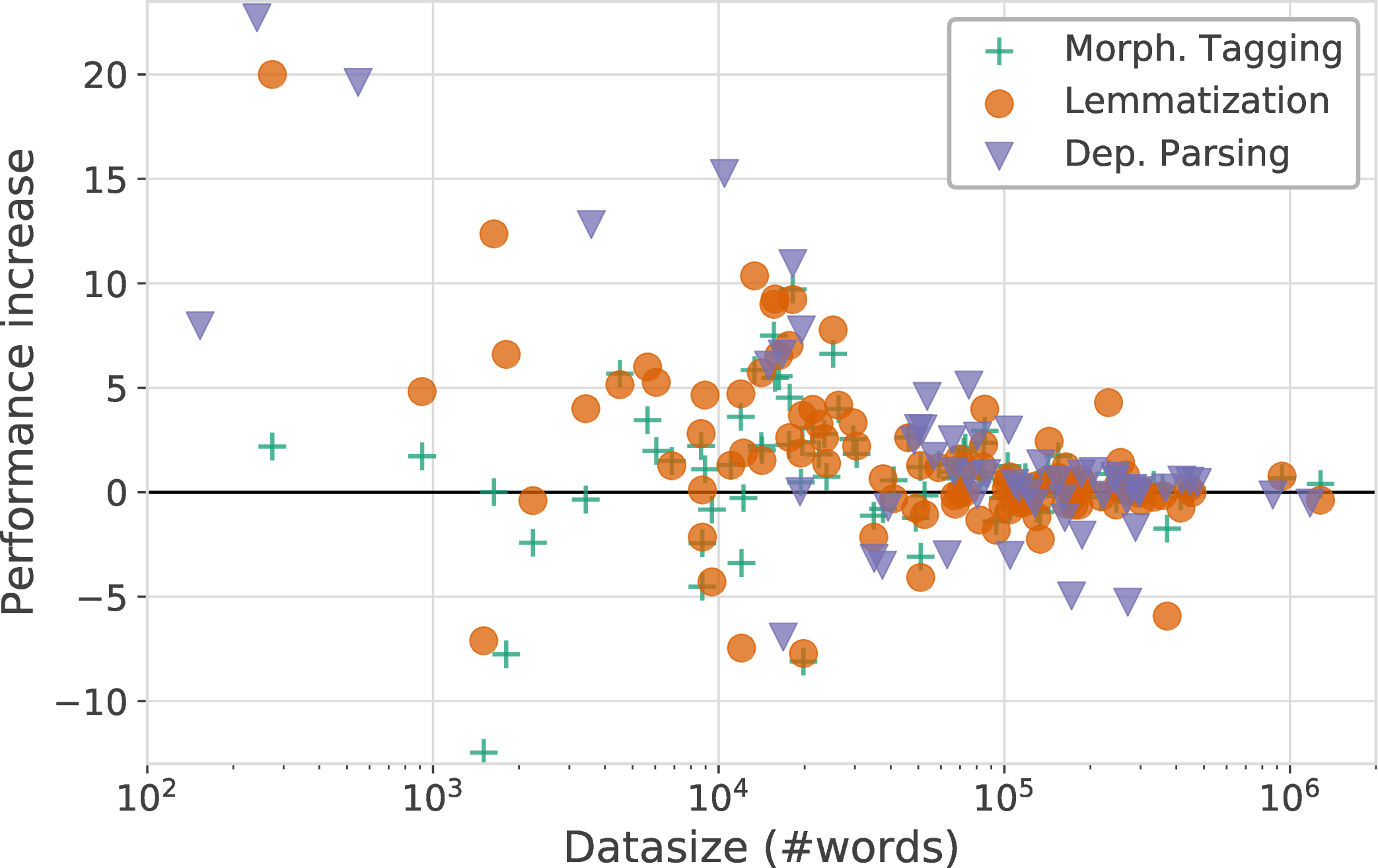
Comparing the mono-lingual dataset groups with the multi-lingual groups, we can see that gold dataset embeddings improve results in both settings for 2/3 tasks. The only setup where gold dataset embeddings are not beneficial is for morphological tagging in multi-lingual groups, where the gains for lemmatization are also only marginal (+0.63 abs.compared to base). This may be attributed to the nature of the tasks, morphological tagging and lemmatization are more language-specific, making it difficult to transfer relevant information from another language. In Figure 2, we plot the performance increase from base to using gold dataset ID’s in relation to its dataset size. Unsurprisingly, the largest gains are obtained in smaller datasets (\(<\)50,000 words) for all tasks. However, especially for the morphological tasks, the largest drops are also observed in this range, and mainly happen for low-resource languages which are paired with a distant language (e.g. Akkadian (akk_pisandub) and Irish (ga_idt)).
3.1.0.3 Gold vs Predicted
The pred columns in Table 1 shows that dataset embeddings are only beneficial (i.e. outperforming base) for lemmatization and dependency parsing when we do not have access to the gold dataset ids but use predicted ids instead. For lemmatization, the average increase compared to base is only 0.31 Acc., whereas for dependency parsing, it is +1.60 LAS. Pred is mostly beneficial in multi-lingual dataset groups, which is probably because the performance of the dataset classifier (Section 2.2) is higher in these cases.
| #src | concat | pred | |
|---|---|---|---|
| All | 53 | 53.80 | 53.87 |
| \(\exists\) same-lang | 35 | 66.35 | 66.62 |
| \(\nexists\) same-lang | 18 | 29.39 | 29.06 |
3.2 Zero-shot evaluation↩︎
In many real-world situations, the basic assumption that data instances originate from the training data distribution is violated, and it becomes essential to find a good way of using data from other sources, like finding the best proxy source. To test whether dataset embeddings are still useful in a zero-shot setup, we perform experiments where we hold out the target dataset during training and then classify all development sentences into the other sets. We run this experiment only for dataset groups containing more than 2 datasets (11 groups and 53 datasets, for dependency parsing). As baseline we compare to a model trained on the concatenation of all other datasets from the group. This zero-shot setup is challenging. Results are expected to be overall lower.
Detailed results are reported in Appendix 7–Table 2 summarizes the main results.6 We aggregate over datasets for which another in-language dataset is available within its dataset group (“\(\exists\) same-lang”), and those where this is not the case. Overall, the performance increase has almost vanished, having only an 0.07 absolute increase in LAS (‘all’). This increase is void in cases no in-language data exists in the group. Only for datasets for which a same language dataset exists (\(\exists\) same-lang, that is, a treebank exists for the language but it comes from another distribution/domain), slight improvements are obtained. We conclude that dataset embeddings are not useful in setups when the test instances are from another distribution.
| In-dataset training | zero-shot | |||||||
| dataset | size | svm | base | concat | gold | pred | concat | pred |
| nl_alp | 186k | 0.96 | 84.10 | 84.41 | 84.97 | 84.74 | 72.03 | 73.69 |
| af_afri | 34k | 1.00 | 79.57 | 78.95 | 79.98 | 80.44 | 35.86 | 34.84 |
| nl_lassy | 75k | 0.88 | 76.76 | 81.59 | 81.89 | 81.52 | 74.70 | 75.48 |
| de_gsd | 268k | 1.00 | 79.76 | 78.96 | 79.39 | 79.35 | 14.30 | 15.09 |
| en_pud | 0 | 0.00 | - | - | - | - | 81.90 | 81.89 |
| en_ewt | 205k | 0.91 | 82.43 | 82.60 | 83.42 | 82.82 | 71.11 | 71.23 |
| en_lines | 50k | 0.77 | 76.15 | 75.06 | 79.20 | 77.14 | 74.71 | 74.68 |
| en_gum | 54k | 0.71 | 78.18 | 80.32 | 82.77 | 80.58 | 80.12 | 79.98 |
3.5pt
For demonstration purposes, we highlight the full results of two dataset groups in Table 3. The first (multi-lingual) group shows that dataset-embeddings are mainly beneficial for languages with multiple datasets, both in the in-domain and zero-shot setting. In this particular dataset group, prediction of the embeddings performs on-par with the gold labels, probably because of the high performance of the classifier. In contrast, in the second (mono-lingual) group, the classifier scores lower, and pred prediction performances are lower compared to gold. For this group, predicted dataset embeddings are outperformed by a simple dataset concatenation.
4 Conclusion↩︎
We provide an extensive evaluation of dataset embeddings in two large-scale settings where they were used successfully [6], [7]. In setups where in-distribution training data is available, we found dataset embeddings more useful in monolingual dataset groups, compared to cross-lingual ones. In general, performance gains were the largest for 1) datasets for which another same-language datasets was available during training 2) small datasets 3) datasets which were part of a large dataset group. However, with predicted id’s, their benefit is limited, contrary to gold information. When moving to zero-shot setups, the performance increases become negligible (except for some particular datasets). In particular, without in-source training data, dataset embeddings work in some cases when another treebank for the language exists; but this gain is not consistent and often small. Overall, we find dataset embeddings fail to be a viable adaptation method when no in-source data is available. Hence, in many realistic out-of-distribution setups, their benefit vanishes.
Acknowledgements↩︎
We would like to thank Gertjan van Noord for feedback on an earlier version of this paper. We thank NVIDIA, the HPC cluster at the ITU and the University of Groningen for computing resources. This research was supported by an Amazon Research Award, an STSM in the Multi3Generation COST action (CA18231), and grant 9063-00077B (Danmarks Frie Forskningsfond).
5 Reproducability report↩︎
The UUParser was run on two E5-2660 v3’s (40 threads total, we used only 30), and took on average approximately 20 hours on a single thread per model. For three random seeds, 16 dataset groups, and approximately 5 settings (4 from Section 3.1 +1 from Section 3.2 were we only used half of the groups in two settings), the total number of models is 240. So the total computation walltime was 160 hours (approximately a week).
The Multi-Team tagger was run on two Tesla V100’s (one model per V100, so two models were trained in parallel). On average this took approximately 3 hours. For this setup we had 104 dataset pairs, of which 82 were unique (if the pairs consist of the same two languages, we only trained one model). For the Multi-Team tagger, we ran four setups (Section 3.1), totaling to 328 models. The total computation time was 984 hours, which divided by 2 gpus resulted in a walltime of 492 hours (approximately three weeks).
Regarding the differences in the settings (base, concat, gold and pred), there were no clear trends in differences in run-time, even the base settings (where multiple models where trained for 1 dataset group) was equal in runtime compared to the other settings where one large model was trained.
It should be noted that the UUParser uses a maximum of 15,000 sentences per epoch, and the Multi-Team tagger 500,000 words (default settings), which makes training times substantially shorter (especially for the UUParser), and reduced the memory usage. Excluding external embeddings helped us reduce the running time and memory usage even further. For the UUParser, a maximum of 8GB ram is enough for training a single model ( 4GB on average), and the Multi-Team tagger requires a minimum of 8GB of GPU RAM.
For all the other settings and hyperparameters, we exactly replicated the original code from the and , and thus refer to their papers for experimental details. The only adaptation we made to the systems is that for the UUParser we added support for supplying the dataset information in the connlu misc-column (the adapted version is available in our repo).
6 Aggregates over all results↩︎
For easier analysis, we provide average scores over aggregates of datasets. To this end, we propose to use data-filters, and report average scores over specific subsets of the data. The results are shown in Table 4. The filters show aggregates over a) whether the training portion of the dataset is small (\(<\) 30,000 words) or large b) whether the dataset group to which this dataset belongs is mono-lingual or multi-lingual c) whether another dataset with the same language is available in the dataset group d) whether the svm classifier predicts the datasource id’s with an accuracy of \(>\)95% accuracy e) whether the word overlap is larger then 10%.
| Language Pairs | Morphological Tagging (F1) | Lemmatization (Accuracy) | Language Clusters | Dependency Parsing (LAS) | |||||||||||||||
| Filtering | #sets | size | WO | svm | base | concat | gold | pred | base | concat | gold | pred | #sets | size | svm | base | concat | gold | pred |
| All | 104 | 121 | 0.31 | 0.95 | 92.04 | 91.43 | 92.75 | 91.85 | 91.10 | 91.02 | 92.55 | 91.41 | 58 | 161 | 0.91 | 72.92 | 74.07 | 75.53 | 74.52 |
| Large | 65 | 186 | 0.28 | 0.94 | 95.40 | 94.78 | 95.72 | 94.98 | 95.92 | 95.08 | 96.00 | 95.19 | 46 | 200 | 0.92 | 80.80 | 79.62 | 80.98 | 80.06 |
| Small | 39 | 13 | 0.35 | 0.98 | 86.46 | 85.85 | 87.78 | 86.65 | 83.07 | 84.24 | 86.79 | 85.11 | 12 | 10 | 0.88 | 42.75 | 52.79 | 54.65 | 53.30 |
| Multi-lang | 45 | 77 | 0.13 | 0.99 | 89.30 | 88.14 | 88.69 | 88.88 | 87.75 | 87.33 | 88.38 | 88.22 | 48 | 163 | 0.92 | 71.35 | 72.87 | 74.03 | 73.32 |
| Single-lang | 59 | 154 | 0.44 | 0.92 | 94.14 | 93.94 | 95.84 | 94.13 | 93.66 | 93.83 | 95.73 | 93.84 | 10 | 149 | 0.86 | 80.48 | 79.84 | 82.74 | 80.29 |
| \(\exists\) same-lang | 59 | 154 | 0.44 | 0.92 | 94.14 | 93.94 | 95.84 | 94.13 | 93.66 | 93.83 | 95.73 | 93.84 | 35 | 187 | 0.86 | 77.32 | 77.33 | 79.29 | 77.76 |
| \(\nexists\) same-lang | 45 | 77 | 0.13 | 0.99 | 89.30 | 88.14 | 88.69 | 88.88 | 87.75 | 87.33 | 88.38 | 88.22 | 23 | 121 | 0.98 | 66.23 | 69.11 | 69.80 | 69.60 |
| pred\(<\)95% | 33 | 177 | 0.41 | 0.87 | 95.15 | 94.05 | 96.45 | 94.24 | 94.57 | 94.12 | 95.77 | 94.24 | 24 | 134 | 0.79 | 73.60 | 75.43 | 78.23 | 76.00 |
| pred\(>\)95% | 71 | 95 | 0.26 | 0.99 | 90.60 | 90.21 | 91.02 | 90.75 | 89.49 | 89.57 | 91.05 | 90.10 | 34 | 179 | 0.99 | 72.45 | 73.11 | 73.62 | 73.48 |
| highWO | 78 | 139 | 0.39 | 0.94 | 93.22 | 92.98 | 94.69 | 93.36 | 92.82 | 93.11 | 94.94 | 93.38 | 58 | 161 | 0.91 | 72.92 | 74.07 | 75.53 | 74.52 |
| lowWO | 26 | 67 | 0.05 | 1.00 | 88.51 | 86.79 | 86.91 | 87.34 | 85.94 | 84.72 | 85.38 | 85.49 | |||||||
7 Full results for dependency parsing↩︎
Table 5 shows the results of the UUParser [7] for each dataset, grouped by dataset groups. All results are the average over three runs. We do not report scores for datasets without in-source training data in the ‘parser setting’ columns (which corresponds to Section 3.1 of the paper), as training data is necessary for those settings.
For the ‘without train’ columns (corresponding to Section 3.2 of the paper), we do not include results for dataset groups of size two; this is because we leave one training set out, and try to predict for the corresponding development set in which set it belongs. For groups of size two, this classification is trivial and non-informative, as there is only one dataset left. The left-out datasets are not taken into account for the averages. The reported results are on development splits, except for datasets which did not have a development split available, there we used test (indicated with * in the table) as we do not perform any tuning.
| In-dataset training | Zero-shot | ||||||||
| cluster | dataset | size | svm | base | concat | gold | pred | concat | pred |
| af-de-nl | nl_alpino | 186,046 | 0.96 | 84.10 | 84.41 | 84.97 | 84.74 | 72.03 | 73.69 |
| af_afribooms | 33,894 | 1.00 | 79.57 | 78.95 | 79.98 | 80.44 | 35.86 | 34.84 | |
| nl_lassysmall | 75,134 | 0.88 | 76.76 | 81.59 | 81.89 | 81.52 | 74.70 | 75.48 | |
| de_gsd | 268,414 | 1.00 | 79.76 | 78.96 | 79.39 | 79.35 | 14.30 | 15.09 | |
| e-sla | uk_iu | 75,098 | 0.99 | 79.86 | 79.49 | 80.63 | 80.53 | 35.69 | 35.99 |
| ru_taiga | 10,479 | 0.35 | 56.47 | 69.32 | 71.73 | 69.30 | 68.81 | 68.81 | |
| ru_syntagrus | 871,521 | 0.99 | 87.26 | 87.07 | 87.13 | 87.24 | 59.52 | 59.34 | |
| en | en_pud | 0 | 0.00 | - | - | - | - | 81.90 | 81.89 |
| en_ewt | 204,607 | 0.91 | 82.43 | 82.60 | 83.42 | 82.82 | 71.11 | 71.23 | |
| en_lines | 50,096 | 0.77 | 76.15 | 75.06 | 79.20 | 77.14 | 74.71 | 74.68 | |
| en_gum | 53,686 | 0.71 | 78.18 | 80.32 | 82.77 | 80.58 | 80.12 | 79.98 | |
| es-ca | ca_ancora | 418,494 | 1.00 | 87.97 | 88.41 | 88.55 | 88.51 | - | - |
| es_ancora | 446,145 | 1.00 | 87.44 | 87.74 | 87.97 | 88.07 | - | - | |
| finno | et_edt | 287,859 | 1.00 | 79.48 | 77.47 | 77.79 | 77.66 | 14.38 | 14.32 |
| fi_tdt | 162,827 | 0.77 | 79.48 | 71.43 | 78.27 | 70.45 | 47.21 | 47.44 | |
| fi_ftb | 127,845 | 0.69 | 79.58 | 70.48 | 79.05 | 70.88 | 51.46 | 52.16 | |
| sme_giella | 16,835 | 1.00 | 63.17 | 53.08 | 56.23 | 55.32 | 6.58 | 6.45 | |
| fi_pud | 0 | 0.00 | - | - | - | - | 74.58 | 74.94 | |
| fr | fr_spoken | 14,952 | 0.93 | 71.39 | 76.15 | 77.48 | 76.72 | 53.50 | 53.35 |
| fr_gsd | 366,372 | 0.96 | 88.23 | 88.09 | 88.43 | 88.30 | 75.65 | 76.36 | |
| fr_sequoia | 51,906 | 0.69 | 85.72 | 85.35 | 88.75 | 87.13 | 80.62 | 80.78 | |
| indic | ur_udtb | 108,690 | 1.00 | 78.15 | 78.43 | 78.58 | 78.58 | - | - |
| hi_hdtb | 281,057 | 1.00 | 89.20 | 89.27 | 89.38 | 89.38 | - | - | |
| iranian | fa_seraji | 122,180 | 1.00 | 82.45 | 82.26 | 82.41 | 82.48 | - | - |
| kmr_mg | 242 | 0.99 | 12.24 | 34.76 | 34.96 | 35.38 | - | - | |
| it | it_isdt | 294,397 | 0.99 | 87.71 | 87.58 | 87.78 | 87.89 | - | - |
| it_postwita | 103,553 | 0.98 | 75.17 | 77.72 | 78.15 | 77.83 | - | - | |
| ko | ko_gsd | 56,687 | 0.68 | 76.70 | 65.62 | 78.42 | 63.56 | - | - |
| ko_kaist | 296,446 | 0.95 | 83.08 | 79.90 | 83.03 | 80.93 | - | - | |
| n-ger | no_nynorsklia | 3,583 | 0.90 | 50.05 | 62.27 | 62.87 | 62.91 | 52.89 | 53.27 |
| fo_oft | 0 | 0.00 | - | - | - | - | 39.57 | 40.87 | |
| sv_talbanken | 66,673 | 0.94 | 77.37 | 76.35 | 78.37 | 77.57 | 70.49 | 71.97 | |
| no_bokmaal | 243,887 | 0.97 | 87.21 | 87.67 | 87.97 | 87.76 | 76.79 | 76.12 | |
| sv_pud | 0 | 0.00 | - | - | - | - | 77.89 | 77.65 | |
| sv_lines | 48,325 | 0.91 | 76.48 | 77.71 | 78.95 | 78.37 | 71.66 | 72.18 | |
| no_nynorsk | 245,330 | 0.98 | 85.67 | 85.49 | 86.27 | 85.93 | 73.50 | 74.36 | |
| da_ddt | 80,378 | 0.97 | 76.97 | 73.79 | 76.84 | 76.06 | 52.04 | 52.27 | |
| old | cu_proiel | 37,432 | 1.00 | 76.62 | 73.91 | 73.12 | 74.22 | 5.36 | 4.95 |
| got_proiel | 35,024 | 1.00 | 71.46 | 69.02 | 68.29 | 69.06 | 8.53 | 8.25 | |
| grc_proiel | 187,049 | 1.00 | 76.09 | 74.32 | 74.03 | 74.35 | 53.90 | 53.51 | |
| la_perseus | 18,184 | 0.88 | 42.55 | 50.45 | 53.51 | 52.61 | 42.61 | 41.12 | |
| la_proiel | 171,928 | 0.99 | 71.18 | 67.03 | 66.22 | 66.94 | 42.68 | 43.68 | |
| grc_perseus | 159,895 | 1.00 | 61.78 | 61.46 | 61.46 | 61.36 | 46.42 | 47.87 | |
| la_ittb | 270,403 | 1.00 | 79.40 | 74.29 | 74.14 | 74.69 | 41.66 | 40.61 | |
| pt-gl | gl_ctg | 86,676 | 0.95 | 80.21 | 79.85 | 81.11 | 80.56 | 63.78 | 64.19 |
| pt_bosque | 222,069 | 1.00 | 87.68 | 87.11 | 87.54 | 87.59 | 49.85 | 50.26 | |
| gl_treegal | 16,707 | 0.62 | 69.15 | 67.24 | 75.76 | 69.03 | 61.62 | 61.71 | |
| sw-sla | sl_sst | 19,473 | 0.96 | 58.65 | 65.65 | 66.42 | 66.31 | 52.06 | 51.81 |
| sr_set | 65,764 | 0.86 | 83.91 | 84.07 | 86.42 | 85.91 | 75.63 | 75.66 | |
| hr_set | 154,055 | 0.94 | 80.66 | 80.22 | 81.23 | 81.07 | 65.74 | 66.08 | |
| sl_ssj | 112,530 | 0.99 | 85.27 | 84.89 | 85.46 | 85.23 | 65.28 | 65.83 | |
| turkic | ug_udt | 19,262 | 1.00 | 61.43 | 60.86 | 61.45 | 60.88 | 1.88 | 2.80 |
| bxr_bdt | 153 | 0.98 | 9.95 | 17.99 | 17.92 | 17.04 | 4.85 | 5.37 | |
| tr_imst | 39,169 | 1.00 | 57.01 | 55.51 | 56.29 | 56.63 | 9.51 | 9.38 | |
| kk_ktb | 547 | 1.00 | 11.54 | 30.52 | 31.16 | 29.14 | 7.03 | 6.19 | |
| w-sla | sk_snk | 80,575 | 0.98 | 80.39 | 82.49 | 83.07 | 82.51 | 59.77 | 59.57 |
| cs_pud | 0 | 0.00 | - | - | - | - | 83.79 | 83.77 | |
| cs_pdt | 1,175,374 | 0.92 | 87.92 | 87.41 | 87.40 | 87.39 | 79.07 | 79.33 | |
| pl_sz | 63,070 | 0.46 | 85.31 | 80.88 | 82.31 | 81.49 | 67.40 | 67.88 | |
| hsb_ufal | 460 | 0.90 | 6.40 | 45.24 | 46.30 | 44.99 | 39.10 | 38.55 | |
| pl_lfg | 104,750 | 0.71 | 90.98 | 86.51 | 87.96 | 87.53 | 70.76 | 70.49 | |
| cs_fictree | 134,059 | 0.78 | 85.77 | 86.92 | 87.14 | 87.08 | 83.75 | 82.91 | |
| cs_cac | 473,622 | 0.83 | 86.86 | 87.40 | 87.32 | 87.40 | 83.73 | 83.57 | |
8 Full results for morphological tagging and lemmatization↩︎
Table 7 shows the results of the Multi-Team tagger [6] on the development data for each dataset. Because of the computational costs, results are over a single run. The second column shows the ‘help-dataset’ that each dataset is paired with, based on word overlap.
Note that data sizes are different compared to Table 5 due to a re-split of the data by [12], and different UD versions ( used 2.3 whereas used 2.2). Another effect of this re-split is that for all datasets, a train, development and test split is available. Also note that dataset prediction (svm) scores reported are on the train data; so if the score is 1.00, pred and gold can still have different scores because the dataset prediction was not equally accurate on the development data.
| Morphological Tagging (F1) | Lemmatization (Accuracy) | |||||||||||
| dataset | additional | size | wo | svm | base | concat | gold | pred | base | concat | gold | pred |
| af_afribooms | nl_alpino | 40,390 | 0.20 | 99.85 | 96.50 | 96.42 | 96.96 | 96.87 | 95.25 | 94.97 | 96.01 | 96.93 |
| akk_pisandub | cs_pdt | 1,505 | 0.02 | 100.00 | 81.96 | 67.99 | 69.49 | 71.96 | 41.33 | 34.67 | 34.22 | 35.11 |
| ar_padt | ar_pud | 231,625 | 0.18 | 96.64 | 95.29 | 95.46 | 96.17 | 95.44 | 90.79 | 91.52 | 95.08 | 91.80 |
| ar_pud | ar_padt | 17,645 | 0.56 | 96.64 | 89.97 | 87.49 | 92.24 | 87.20 | 77.36 | 62.83 | 84.39 | 57.39 |
| be_hse | ru_syntagrus | 6,855 | 0.08 | 99.98 | 80.51 | 80.61 | 82.01 | 83.49 | 78.48 | 75.67 | 79.75 | 81.58 |
| bg_btb | ru_syntagrus | 133,659 | 0.12 | 99.60 | 97.85 | 96.67 | 96.89 | 96.97 | 96.95 | 94.54 | 94.70 | 94.95 |
| bm_crb | cs_pdt | 12,025 | 0.09 | 99.98 | 94.03 | 89.49 | 90.64 | 89.92 | 87.86 | 78.40 | 80.40 | 80.09 |
| br_keb | no_bokmaal | 8,772 | 0.07 | 99.87 | 90.89 | 90.53 | 88.45 | 89.67 | 88.75 | 89.77 | 88.86 | 88.35 |
| bxr_bdt | ru_syntagrus | 8,770 | 0.04 | 99.94 | 83.46 | 80.65 | 78.94 | 79.96 | 82.71 | 80.65 | 80.56 | 81.63 |
| ca_ancora | es_ancora | 441,014 | 0.18 | 99.71 | 98.61 | 98.48 | 98.57 | 98.56 | 98.35 | 98.42 | 98.56 | 98.69 |
| cs_cac | cs_pdt | 414,810 | 0.57 | 90.62 | 97.19 | 96.71 | 96.98 | 96.72 | 98.03 | 97.05 | 97.27 | 97.24 |
| cs_cltt | cs_pdt | 29,549 | 0.81 | 99.87 | 94.62 | 96.65 | 97.16 | 96.62 | 94.02 | 97.56 | 97.35 | 97.56 |
| cs_fictree | cs_pdt | 143,508 | 0.58 | 95.01 | 95.89 | 94.89 | 96.54 | 95.36 | 95.21 | 97.07 | 97.65 | 97.15 |
| cs_pdt | cs_cac | 1,278,252 | 0.27 | 90.62 | 96.65 | 96.78 | 97.05 | 96.76 | 97.50 | 97.10 | 97.12 | 97.19 |
| cs_pud | cs_pdt | 15,614 | 0.79 | 98.98 | 87.38 | 96.26 | 94.88 | 96.38 | 87.03 | 96.84 | 96.03 | 97.00 |
| cu_proiel | ru_syntagrus | 50,963 | 0.04 | 99.98 | 94.71 | 92.94 | 91.62 | 92.12 | 95.17 | 92.66 | 91.09 | 91.28 |
| da_ddt | no_bokmaal | 85,373 | 0.25 | 97.38 | 92.58 | 95.21 | 95.52 | 95.26 | 92.27 | 95.60 | 96.25 | 95.30 |
| de_gsd | fr_gsd | 246,633 | 0.06 | 99.94 | 93.48 | 92.18 | 93.16 | 93.05 | 96.55 | 94.95 | 95.94 | 95.60 |
| el_gdt | grc_proiel | 52,583 | 0.04 | 99.96 | 96.51 | 96.25 | 96.36 | 96.45 | 95.00 | 94.52 | 93.93 | 95.15 |
| en_ewt | en_gum | 218,154 | 0.30 | 89.27 | 95.73 | 95.75 | 95.49 | 95.32 | 97.02 | 96.79 | 96.81 | 96.46 |
| en_gum | en_ewt | 67,381 | 0.57 | 89.27 | 94.45 | 94.39 | 95.11 | 94.29 | 96.94 | 93.94 | 96.37 | 94.63 |
| en_lines | en_ewt | 70,079 | 0.56 | 91.20 | 95.14 | 93.33 | 95.88 | 94.71 | 97.39 | 94.98 | 97.34 | 96.59 |
| en_partut | en_ewt | 40,974 | 0.63 | 95.66 | 93.45 | 90.75 | 94.03 | 91.83 | 97.58 | 96.53 | 97.27 | 95.83 |
| en_pud | en_ewt | 17,727 | 0.68 | 95.14 | 90.87 | 95.08 | 95.40 | 94.91 | 93.55 | 95.62 | 96.17 | 94.68 |
| es_ancora | es_gsd | 454,069 | 0.47 | 87.10 | 98.34 | 97.46 | 98.48 | 97.97 | 98.60 | 97.15 | 98.59 | 97.80 |
| es_gsd | es_ancora | 358,355 | 0.42 | 87.10 | 97.35 | 96.15 | 97.55 | 96.97 | 98.59 | 95.81 | 98.43 | 97.65 |
| et_edt | cs_pdt | 371,564 | 0.02 | 99.75 | 96.60 | 94.65 | 94.86 | 94.68 | 94.73 | 89.62 | 88.80 | 89.09 |
| eu_bdt | es_ancora | 104,530 | 0.05 | 99.96 | 95.10 | 93.62 | 94.41 | 94.38 | 96.32 | 95.35 | 95.47 | 95.52 |
| fa_seraji | ur_udtb | 127,371 | 0.12 | 100.00 | 97.15 | 97.24 | 97.26 | 97.31 | 95.00 | 94.24 | 95.29 | 94.97 |
| fi_ftb | fi_tdt | 142,514 | 0.37 | 71.46 | 95.25 | 94.94 | 96.18 | 94.94 | 92.15 | 90.99 | 92.75 | 90.85 |
| fi_pud | fi_tdt | 13,356 | 0.49 | 94.58 | 91.56 | 96.97 | 97.41 | 96.81 | 78.62 | 86.06 | 88.98 | 86.78 |
| fi_tdt | fi_ftb | 173,899 | 0.30 | 71.46 | 96.54 | 95.32 | 97.07 | 95.18 | 92.42 | 90.27 | 92.22 | 90.03 |
| fo_oft | no_nynorsk | 8,960 | 0.12 | 99.83 | 90.36 | 86.49 | 91.46 | 90.38 | 83.87 | 81.59 | 88.52 | 86.66 |
| fr_gsd | fr_sequoia | 333,477 | 0.15 | 93.23 | 97.71 | 97.65 | 98.07 | 97.40 | 97.74 | 96.52 | 97.50 | 96.14 |
| fr_partut | fr_gsd | 23,443 | 0.82 | 97.28 | 94.72 | 96.33 | 97.51 | 96.13 | 94.20 | 95.13 | 96.78 | 95.10 |
| fr_sequoia | fr_gsd | 58,963 | 0.66 | 93.23 | 96.74 | 96.79 | 98.07 | 96.21 | 96.99 | 96.90 | 98.17 | 95.81 |
| fr_spoken | fr_gsd | 30,410 | 0.77 | 99.33 | 95.81 | 97.10 | 97.64 | 97.44 | 96.77 | 98.79 | 98.98 | 99.07 |
| ga_idt | cs_pdt | 19,812 | 0.04 | 99.95 | 83.38 | 76.03 | 75.27 | 77.94 | 84.63 | 76.48 | 76.91 | 79.01 |
| gl_ctg | es_ancora | 114,228 | 0.40 | 99.88 | 97.33 | 97.22 | 97.38 | 97.36 | 98.12 | 98.14 | 98.16 | 98.37 |
| gl_treegal | gl_ctg | 21,366 | 0.53 | 92.26 | 91.56 | 82.76 | 94.64 | 84.77 | 92.69 | 94.69 | 96.66 | 95.57 |
| got_proiel | no_nynorsk | 48,980 | 0.01 | 99.91 | 95.20 | 94.61 | 93.97 | 93.94 | 95.35 | 94.60 | 94.58 | 94.23 |
| grc_perseus | grc_proiel | 173,299 | 0.25 | 99.95 | 94.86 | 94.74 | 95.05 | 95.05 | 93.24 | 92.67 | 93.15 | 93.19 |
| grc_proiel | grc_perseus | 185,142 | 0.31 | 99.95 | 96.92 | 96.98 | 97.08 | 97.11 | 95.85 | 95.90 | 96.46 | 96.30 |
| he_htb | ru_gsd | 134,397 | 0.00 | 100.00 | 96.26 | 96.17 | 96.07 | 96.23 | 96.62 | 96.52 | 96.44 | 96.71 |
| hi_hdtb | mr_ufal | 295,265 | 0.01 | 100.00 | 96.70 | 96.87 | 96.77 | 96.89 | 98.57 | 98.34 | 98.52 | 98.40 |
| hr_set | sr_set | 164,557 | 0.28 | 88.98 | 95.14 | 94.85 | 95.50 | 94.59 | 95.81 | 94.53 | 95.25 | 94.52 |
| hsb_ufal | cs_pdt | 9,475 | 0.08 | 99.95 | 79.92 | 77.49 | 79.09 | 76.84 | 82.68 | 74.70 | 78.39 | 76.76 |
| hu_szeged | et_edt | 34,903 | 0.03 | 99.95 | 92.27 | 91.05 | 91.15 | 89.75 | 90.09 | 88.37 | 87.94 | 84.66 |
| hy_armtdp | ru_pud | 19,419 | 0.00 | 100.00 | 90.34 | 91.31 | 90.81 | 91.13 | 90.00 | 92.15 | 91.87 | 92.01 |
| id_gsd | es_gsd | 101,687 | 0.11 | 99.92 | 92.72 | 92.87 | 93.30 | 93.39 | 98.77 | 98.87 | 98.97 | 98.81 |
| it_isdt | it_partut | 250,714 | 0.28 | 79.42 | 98.07 | 97.91 | 98.26 | 97.77 | 97.52 | 96.70 | 97.87 | 96.85 |
| it_partut | it_isdt | 46,228 | 0.94 | 79.42 | 96.11 | 98.47 | 98.73 | 98.30 | 96.07 | 97.78 | 98.68 | 97.21 |
| it_postwita | it_isdt | 104,437 | 0.46 | 98.49 | 95.76 | 96.13 | 96.15 | 96.53 | 94.15 | 96.14 | 94.89 | 95.20 |
| it_pud | it_isdt | 19,634 | 0.69 | 94.02 | 94.30 | 85.62 | 96.69 | 84.00 | 93.32 | 96.64 | 97.00 | 95.22 |
| ja_gsd | ja_pud | 154,453 | 0.14 | 92.59 | 94.59 | 96.10 | 96.31 | 95.96 | 98.06 | 98.81 | 98.77 | 98.77 |
| ja_modern | ja_gsd | 12,213 | 0.29 | 99.78 | 95.93 | 95.69 | 95.65 | 95.86 | 93.67 | 95.96 | 95.55 | 96.59 |
| ja_pud | ja_gsd | 22,450 | 0.64 | 92.59 | 95.85 | 97.91 | 97.66 | 97.29 | 96.08 | 99.30 | 99.34 | 99.01 |
| kmr_mg | es_gsd | 8,680 | 0.03 | 100.00 | 86.43 | 86.93 | 88.64 | 87.61 | 88.38 | 90.72 | 91.19 | 90.44 |
| ko_gsd | ko_kaist | 69,382 | 0.33 | 92.29 | 93.53 | 86.94 | 94.97 | 87.35 | 89.88 | 89.30 | 91.47 | 85.59 |
| ko_kaist | ko_gsd | 302,384 | 0.12 | 92.29 | 95.86 | 95.48 | 95.97 | 95.39 | 94.30 | 94.20 | 93.88 | 92.37 |
| ko_pud | ko_kaist | 14,106 | 0.55 | 97.97 | 93.41 | 82.62 | 95.62 | 83.29 | 92.36 | 75.41 | 98.08 | 75.41 |
| kpv_ikdp | ru_syntagrus | 916 | 0.26 | 99.95 | 61.38 | 48.34 | 63.10 | 55.79 | 56.63 | 55.42 | 61.45 | 61.45 |
| kpv_lattice | ru_syntagrus | 1,805 | 0.09 | 99.96 | 75.26 | 66.32 | 67.50 | 67.36 | 57.69 | 58.24 | 64.29 | 61.54 |
| la_ittb | la_proiel | 298,460 | 0.37 | 99.98 | 97.08 | 97.23 | 97.03 | 97.36 | 98.54 | 97.98 | 98.65 | 98.54 |
| la_perseus | la_proiel | 25,157 | 0.49 | 99.89 | 82.04 | 87.64 | 88.67 | 87.95 | 80.99 | 87.44 | 88.76 | 87.37 |
| la_proiel | la_ittb | 174,977 | 0.20 | 99.98 | 95.30 | 95.15 | 94.83 | 95.10 | 96.65 | 94.54 | 96.03 | 95.47 |
| lt_hse | lv_lvtb | 4,511 | 0.05 | 99.83 | 72.44 | 77.53 | 78.12 | 77.94 | 72.96 | 77.25 | 78.11 | 77.68 |
| lv_lvtb | hr_set | 129,982 | 0.02 | 99.81 | 95.13 | 94.58 | 94.34 | 94.54 | 93.78 | 93.41 | 92.60 | 93.85 |
| mr_ufal | hi_hdtb | 3,427 | 0.16 | 100.00 | 76.63 | 77.98 | 76.28 | 78.61 | 70.12 | 72.47 | 74.12 | 72.00 |
| nl_alpino | nl_lassysmall | 178,169 | 0.23 | 93.27 | 95.88 | 95.49 | 96.18 | 95.98 | 95.60 | 94.57 | 95.61 | 95.43 |
| nl_lassysmall | nl_alpino | 84,612 | 0.41 | 93.27 | 93.67 | 95.15 | 96.04 | 95.60 | 93.34 | 94.24 | 95.61 | 94.99 |
| no_bokmaal | no_nynorsk | 264,958 | 0.24 | 96.34 | 97.24 | 97.41 | 97.25 | 97.65 | 98.23 | 97.86 | 98.31 | 98.01 |
| no_nynorsk | no_bokmaal | 255,088 | 0.25 | 96.34 | 96.68 | 97.10 | 97.03 | 97.31 | 96.59 | 97.50 | 98.02 | 97.66 |
| no_nynorsklia | no_nynorsk | 11,959 | 0.65 | 99.18 | 92.16 | 95.44 | 95.77 | 95.11 | 92.93 | 98.09 | 97.64 | 97.72 |
| pcm_nsc | en_ewt | 11,038 | 0.74 | 99.99 | 92.95 | 93.28 | 94.26 | 94.15 | 98.55 | 99.92 | 99.84 | 99.76 |
| pl_lfg | pl_sz | 118,526 | 0.41 | 60.73 | 95.71 | 94.43 | 96.43 | 93.91 | 95.93 | 94.67 | 95.49 | 94.96 |
| pl_sz | pl_lfg | 73,011 | 0.53 | 60.73 | 92.68 | 88.62 | 94.82 | 89.33 | 95.78 | 93.96 | 95.79 | 94.81 |
| pt_bosque | pt_gsd | 188,265 | 0.48 | 87.08 | 96.38 | 88.48 | 96.84 | 92.15 | 97.43 | 86.31 | 97.84 | 90.18 |
| pt_gsd | pt_bosque | 265,352 | 0.41 | 87.08 | 97.63 | 94.92 | 98.03 | 93.49 | 97.53 | 94.37 | 98.36 | 94.38 |
| ro_nonstandard | ro_rrt | 164,375 | 0.24 | 97.63 | 95.19 | 95.83 | 95.55 | 96.14 | 94.49 | 96.06 | 95.71 | 96.02 |
| ro_rrt | ro_nonstandard | 182,366 | 0.11 | 97.63 | 97.25 | 97.16 | 97.19 | 97.30 | 97.09 | 97.11 | 96.47 | 97.36 |
| ru_gsd | ru_syntagrus | 84,013 | 0.55 | 96.08 | 93.72 | 91.02 | 94.67 | 91.26 | 95.69 | 91.96 | 96.90 | 92.36 |
| ru_pud | ru_syntagrus | 16,233 | 0.74 | 98.69 | 88.38 | 87.34 | 93.93 | 87.87 | 86.92 | 94.09 | 93.46 | 93.51 |
| ru_syntagrus | ru_gsd | 937,395 | 0.13 | 96.08 | 96.69 | 96.84 | 97.36 | 96.40 | 96.73 | 96.42 | 97.50 | 95.68 |
| ru_taiga | ru_syntagrus | 18,173 | 0.66 | 98.05 | 82.67 | 92.42 | 92.38 | 92.23 | 83.24 | 92.07 | 92.47 | 92.98 |
| sa_ufal | hi_hdtb | 1,634 | 0.10 | 99.98 | 69.59 | 68.81 | 69.60 | 70.68 | 52.58 | 62.89 | 64.95 | 66.49 |
| sk_snk | cs_pdt | 93,740 | 0.22 | 99.22 | 94.69 | 92.39 | 93.30 | 93.51 | 95.13 | 91.31 | 93.31 | 92.61 |
| sl_ssj | hr_set | 118,536 | 0.12 | 99.33 | 95.38 | 94.98 | 95.09 | 95.65 | 96.13 | 95.58 | 95.97 | 96.32 |
| sl_sst | sl_ssj | 26,309 | 0.55 | 99.20 | 89.49 | 92.91 | 93.47 | 93.75 | 91.76 | 95.64 | 95.93 | 96.38 |
| sme_giella | no_nynorsk | 23,877 | 0.02 | 99.89 | 91.20 | 90.44 | 91.94 | 91.85 | 87.31 | 86.19 | 88.69 | 88.69 |
| sr_set | hr_set | 72,045 | 0.62 | 88.98 | 95.52 | 95.24 | 97.47 | 96.09 | 95.77 | 95.96 | 97.02 | 95.96 |
| sv_lines | sv_talbanken | 67,016 | 0.31 | 90.90 | 94.33 | 94.98 | 95.30 | 95.14 | 95.29 | 94.73 | 95.12 | 94.57 |
| sv_pud | sv_talbanken | 15,758 | 0.39 | 93.08 | 89.65 | 93.78 | 95.12 | 94.20 | 83.86 | 88.30 | 93.11 | 90.35 |
| sv_talbanken | sv_lines | 82,088 | 0.25 | 90.90 | 96.28 | 96.62 | 96.97 | 96.81 | 96.67 | 95.93 | 95.34 | 95.41 |
| tl_trg | es_gsd | 274 | 0.13 | 99.98 | 74.73 | 82.22 | 76.92 | 83.15 | 60.00 | 72.00 | 80.00 | 76.00 |
| tr_imst | tr_pud | 50,925 | 0.13 | 93.10 | 92.59 | 90.83 | 93.79 | 90.79 | 92.94 | 92.57 | 94.22 | 92.20 |
| tr_pud | tr_imst | 14,180 | 0.33 | 93.10 | 91.82 | 86.88 | 93.83 | 87.66 | 84.80 | 84.92 | 86.32 | 84.34 |
| uk_iu | ru_syntagrus | 98,865 | 0.10 | 99.55 | 92.69 | 91.14 | 92.41 | 92.13 | 93.67 | 91.59 | 93.07 | 92.86 |
| ur_udtb | fa_seraji | 114,786 | 0.16 | 100.00 | 91.69 | 91.30 | 91.64 | 91.40 | 96.20 | 95.51 | 95.68 | 95.93 |
| vi_vtb | en_ewt | 37,637 | 0.02 | 99.87 | 89.82 | 88.84 | 89.02 | 89.39 | 99.18 | 99.83 | 99.83 | 99.90 |
| yo_ytb | es_gsd | 2,238 | 0.06 | 99.99 | 87.46 | 89.49 | 85.04 | 91.00 | 94.00 | 95.20 | 93.60 | 96.00 |
| yue_hk | zh_gsd | 5,641 | 0.42 | 99.93 | 86.32 | 87.42 | 89.77 | 88.27 | 92.97 | 98.97 | 98.97 | 98.97 |
| zh_cfl | zh_gsd | 6,048 | 0.34 | 99.93 | 86.15 | 88.92 | 88.13 | 89.72 | 91.00 | 95.57 | 96.26 | 95.98 |
| zh_gsd | ja_gsd | 102,731 | 0.15 | 99.99 | 89.62 | 91.40 | 90.87 | 91.24 | 98.46 | 99.05 | 98.97 | 99.09 |
| Average | 121,049 | 0.31 | 95.42 | 92.04 | 91.43 | 92.75 | 91.85 | 91.10 | 91.02 | 92.55 | 91.41 |
9 PCA-analysis of gold versus predicted treebank embeddings↩︎
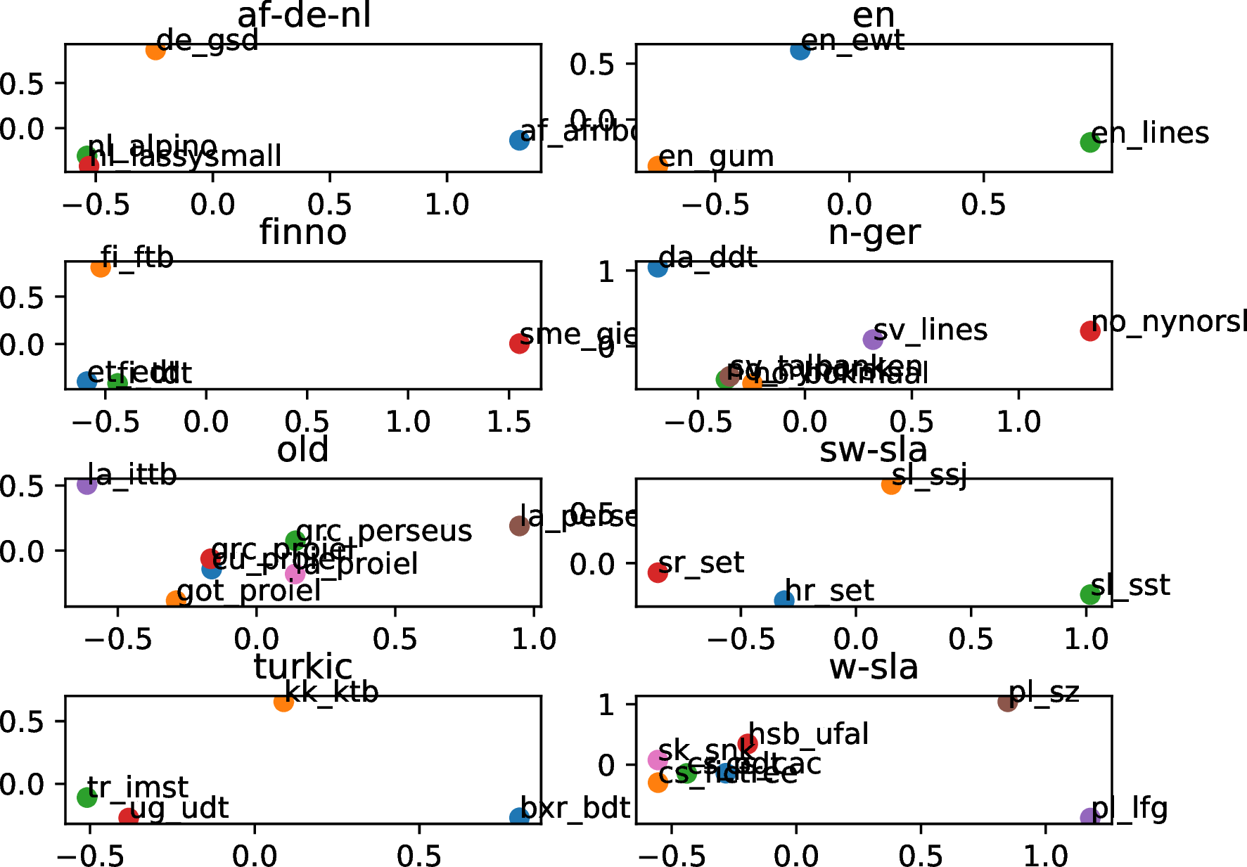
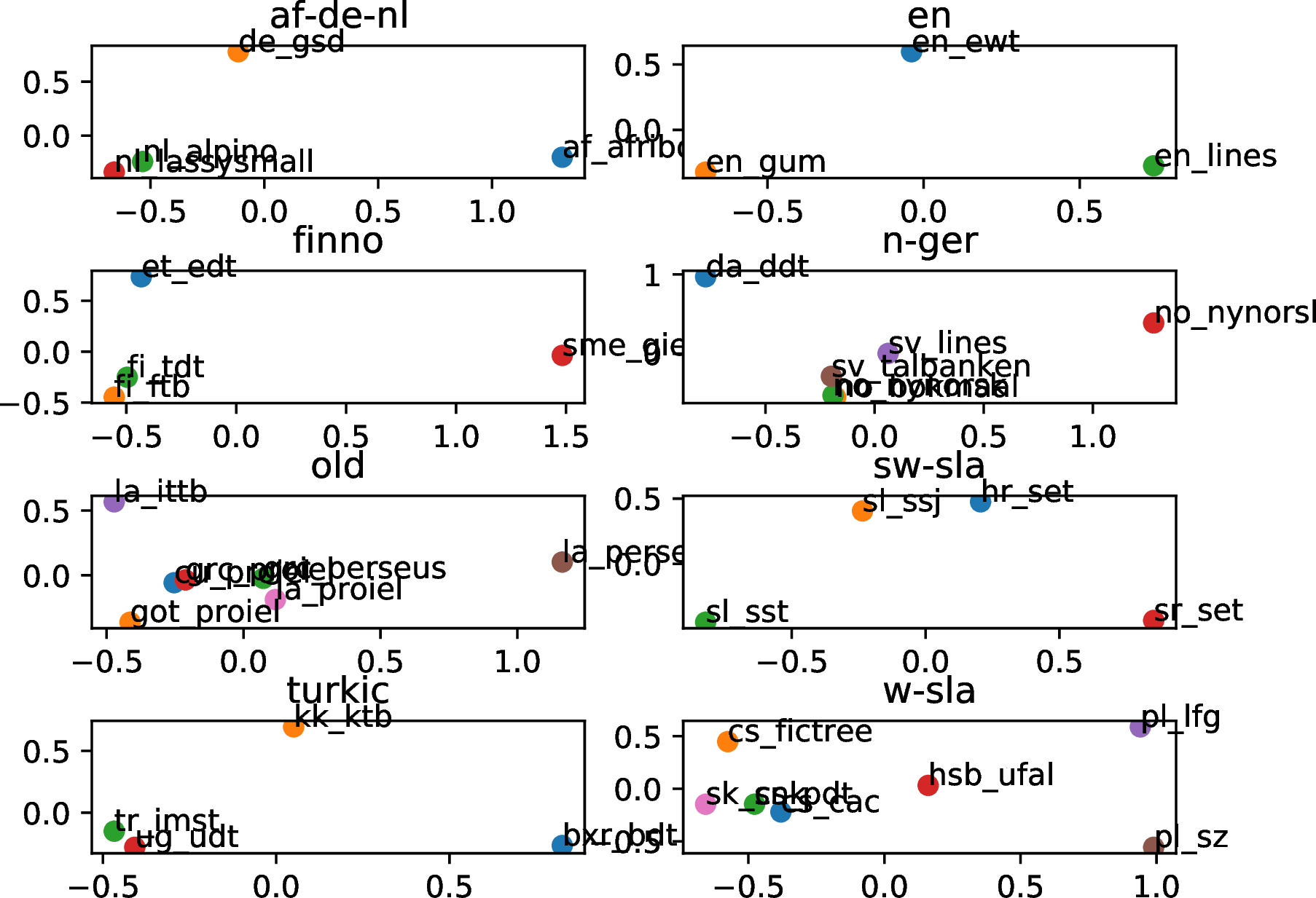
To gain deeper insights in what is represented in treebank embeddings, we plotted the eight largest dataset groups of the UUParser setup into a PCA space [23]. This is done with the default sklearn settings [24]. Results of the gold spaces are shown in Figure 3 and the predicted spaces are plotted in Figure 4. For some groups, there are some clear differences, however for others the plots are highly similar. There seems to be no clear trend in the amount of differences and the performance shifts in Table 5.
References↩︎
source code is available at: https://bitbucket.org/robvanderg/dataembs/src↩︎
More recently, [4] showed that embedding the language can also be beneficial for training contextualized embeddings with masked language modeling.↩︎
showed that performance gains from external embeddings are highly complementary to performance gains from dataset embeddings.↩︎
However, and have shown the usefulness of word-level language labels for processing code-switched data.↩︎
Note that base and gold are not reported here, because no data from the target dataset is included in this experiments.↩︎