1 Introduction and Earlier Work↩︎

In recent years there has been a revival of interest in exploring analogues of back-propagation which could be more biologically plausible than back-propagation, for which concerns were voiced early on [1]. This paper introduces ideas and mathematical derivations for a family of such biologically motivated analogues, in line with earlier work on "target propagation" [2]–[8], in which a feedback path provides targets for each layer, and each layer-to-layer forward and feedback paths form an auto-encoder, respectively with its feedforward path encoder and corresponding feedback path decoder. This paper attempts to provide a solid theoretical foundation for target propagation by studying the case where one can use the auto-encoder to approximately invert the targets of the next layer (\(l\)) in order to obtain a target for the previous layer (\(l-1\)).

See [8] for a review of alternatives or analogues of backpropagation aimed at bridging the gap between backpropgation and biology, and in particular of how target propagation and difference target propagation [7] could potentially be implemented in the brain. The main concerns about a biological implementation of back-propagation can be summarized as follows:

1. The weight transport or weight symmetry problem is that back-propagation requires the backprop calculation (going backwards from outputs towards inputs) to use the exact same weight matrices (transposed) as those used for the forward propagation, but these identical synaptic weights would have to be on different neurons.

2. The non-linearities used in the forward and backward phase of backpropagation are not of the same type and in addition those on the backward path need to be numerically coordinated with the corresponding ones in the forward path (since they should multiply their input by the first derivative of the corresponding forward non-linearities).

3. The brain has recurrent connections (both feedback and lateral ones) which do not disappear while the signals travel on the feedforward paths.

4. Backpropagation needs a clean separation between examples and between the forward phase and backward phase, with the forward phase activations somehow being held while the backward phase proceeds because a combination forward phase and backward phase quantities is needed to perform the synaptic weight updates. Various analogues of backpropagation such as difference target propagation and the proposal made here require a form of time-multiplexing and synchronization in order to separate the feedforward and feedback phases, while the brain seems to use feedback paths all the time.

5. Dale’s law constrains the signs of the synaptic weights (depending on the neuron type), while they are unconstrained in most artificial neural network implementations, including those aiming at biological plausibility.

6. Neurons communicate with spikes, not with real values.

7. Backpropagating through time (BPTT, used to handle recurrent networks) requires (a) storing all past states of the brain and (b) traversing these states backwards to compute updates (c) waiting for a long time before making these updates (to be able to capture sufficiently long dependencies). Instead, the brain seems to make online updates (or possibly daily updates for longer-term consolidation during sleep).

This paper (and target propagation in general) helps with the problem (1) of weight symmetry or weight transport [1], [9], [10], the problem (2) of having to match non-linearities as well, the problem (3) of explaining (to some extent) the feedback and lateral recurrence, and it suggests a way to deal with the problem (4) of synchronization and phases (using neuromodulating gating, e.g., with acetylcholine). This paper does not discuss spiking (but rates can approximately be obtained in various ways by averaging over time and groups of neurons), Dale’s law nor BPTT.

Many other approaches have been proposed to deal with the weight transport problem, notably feedback alignment [11], by showing exact transposes are not always needed (although the approach is still challenged by more complex tasks like ImageNet object recognition [12]). This is in addition to target propagation approaches [3], [6]–[8], [13], which train auto-encoders to obtain feedback weights. Like many other approaches with a feedback path, the approach discussed here assumes that the feedback path mainly influences the computation of targets for the feedforward path. However, variations proposed here use the recurrent computation to settle to approximate inverses of the output target at each layer (so that moving the feedforward activations to these targets would produce the desired output on the final layer). Like Equilibrium Propagation [14], this paper addresses the potential mismatch of non-linearities between the forward and backward phase, here by appropriately training or iterating over the feedback paths (whereas Equilibrium Propagation takes advantage of the propagation of perturbations in the dynamics of a recurrent network with a static input). Like Equilibrium Propagation, the proposed iterative procedure for target propagation is a relaxation, but one that provably converges exponentially fast, with a rate depending on the reconstruction ability of the auto-encoder (hence the need to train the feedback weights), and it avoids the weight transport problem associated with Equilibrium Propagation. Like  [15], this paper proposes to use iterative refinements involving the encoder and decoder at each layer to obtain and then propagate approximate inverses, although [15] use fixed random feedback weights whereas we use a mechanism that requires trained feedback weights (minimizing a reconstruction error) in order to achieve fast convergence to a good inverse. Finally, this paper borrows the idea from GAIT-prop [16] that the targets propagated in target propagation should be only small perturbations of the corresponding feedforward activations to facilitate an analysis of the algorithm based on a linearization of the forward propagation around the forward phase computation. In comparison to GAIT-prop, this paper avoids a potentially exponential growth of required learning rates as one considers layers further from the output, and the proposed update rule is justified and derived in a different way, although also starting from the premise of approximate inverses being computable (in our case via auto-encoder iterations extending the original idea in difference target propagation).

2 Layer-wise approximate inverse↩︎

We focus for now on a multi-layer feedforward model and assume that all the layers have the same size, to make the layer-wise inversion feasible and simple. See [15] for ways to generalize target-propagation methods to the case of unequal layer sizes. See also Section 9.3 to deal with skip connections and architectures which are not structured as a chain. Each layer’s forward phase activation \(h_l\) is computed with its encoder \(f_l\): \[\begin{align} h_l = f_l(h_{l-1}) \end{align}\] where \(f_l\) is implicitly parametrized by \(W_l\), the parameters (weights and biases) used for computing the output of layer \(l\), \(h_0=x\) is the input vector and \(h_L\) is the output layer, with loss \(L(h_L,y)\). The second notation is convenient to describe compositions of these layer-wise functions, so \[\begin{align} h_L = (f_L \circ f_{L-1} \circ \ldots f_1)(x). \end{align}\]

In addition to learning the feedforward weights \(W\), we consider neural networks with a separate feedback path with top-down layers \(g_l\) and corresponding feedback parameters \(\Omega _l\) to compute an approximate inverse of \(f_l\): \[\begin{align} \label{eq:approx-inverse} f_l(g_l(h_{l})) &\approx h_l \nonumber \\ g_l(f_l(h_{l-1})) &\approx h_{l-1}. \end{align}\tag{1}\] Note that inverses compose, so \[\begin{align} (f_L \circ f_{L-1} \circ \ldots \circ f_l) \circ (g_l \circ g_{l+1} \circ \ldots g_L) (h_L) \approx h_L \end{align}\] and simple target propagation starting at \(\tau_L\) (normally chosen close to \(h_L\)) gives rise to \[\begin{align} \tau_l = (g_{l+1} \circ \ldots g_L)(\tau_L) \end{align}\] or equivalently, applying a change \(\tau_l-h_l\) on layer activations \(h_l\) (to give new values \(\tau_l\)) would lead to \[\begin{align} \label{eq:recovering-output-delta} (f_L \circ f_{L-1} \circ f_{l+1})(\tau_l) \approx \tau_L \end{align}\tag{2}\] which would change \(h_L\) in the direction of the gradient of the loss on the output. Note that the inverse condition is achieved when we minimize reconstruction error in the output space (applying the decoder and then the encoder), which is the opposite of the usual auto-encoder reconstruction error (where we apply the encoder and then the decoder). However, the iterative inversion scheme of Section 6 uses the regular auto-encoder property of \(g_l \circ f_l\) being close to the identity, and the version in Section 10 minimizes the reconstruction error of \(g_l \circ f_l\) but obtains \(\tau_{l-1} \rightarrow f_l^{-1}(\tau_l)\) iteratively.

We will assume that \(g\) has enough capacity for approximating the inverse of \(f\). For example it may need an extra hidden layer or use powerful non-linearities assumed to exist in dendritic computation in order to obtain the required flexibility, or the use of iterative refinements to correct the input or output of the decoder in order to approximate the inverse well, as per Sections 5 and 6. A training objective for enforcing the above also needs to be defined (such as squared error on reconstructing pre-activation values).

3 Differential Target-Prop when a Single Layer is Changing↩︎

We will first study the case where a single layer \(l\) is to have its weights updated in order to make the output \(h_L\) match the target output \(\tau_L\). We will also define differential targets \(\tau_l\) for each layer, i.e., small perturbations of the forward activations of each layer obtained by applying and composing the approximate inverses \(g_l\) on the differential output target \(\tau_L\): \[\begin{align} \label{eq:target-prop} \tau_L &= h_L - \beta \frac{\partial L(h_L,y)}{\partial h_L}^T \nonumber \\ \tau_l &= g_{l+1}(\tau_{l+1}) = (g_{l+1}\circ \ldots \circ g_L)(\tau_L) \end{align}\tag{3}\] where \(0<\beta\ll 1\) is a small positive constant: small enough to linearize \(g\) and \(f\) and large enough to make computations with limited precision feasible (which possibly may require several neurons to represent a single quantity with enough precision, in the brain).

Because of the availability of an approximate inverse, we can propagate targets and obtain \(\tau_l\) for layer \(l\) using Eq. 3 . It has the property that if \(h_l\) moves to \(\tau_l\), we obtain \(\tau_L\) as output: \[\begin{align} \label{eq:taul-yields-tauL} (f_L \circ f_{L-1} \circ f_{l+1})(\tau_l) & \approx \tau_L \nonumber \\ L((f_L \circ f_{L-1} \circ f_{l+1})(\tau_l),y) & \approx L(h_L - \beta \frac{\partial L(h_L,y)}{\partial h_L}^T,y) \nonumber \\ &\approx L(h_L,y) - \beta||\frac{\partial L(h_L,y)}{\partial h_L}||^2 \leq L(h_L,y) \end{align}\tag{4}\] for \(\beta\) small enough (it acts like a learning rate). We can move parameters \(W_l\) so that \(h_l\) approaches \(\tau_l\) by considering \(\tau_l\) as a local target for \(h_l\), e.g., using what we now call the single layer update Differential Target-Prop (DTP1) update, either by moving activations \[\begin{align} \Delta_{\rm DTP1} h_l = \tau_l-h_l \end{align}\] or with parameter updates (where the update differs from difference target propagation and other proposals which do not have the normalization factor below): \[\begin{align} \label{eq:delta-dtp} \Delta_{\rm DTP1} W_l = \frac{\partial h_l}{\partial W_l}^T \left( \frac{\partial h_l}{\partial W_l} \frac{\partial h_l}{\partial W_l}^T \right)^{-1} (\tau_l-h_l). \end{align}\tag{5}\] The inverse in the above expression is a normalization factor which goes beyond the usual gradient of the squared error \((\tau_l - h_l)^2\) with respect to \(W_l\), computed by the rest of the expression. The role of this inverse matrix is to make sure that when we apply \(\Delta_{\rm DTP1} W_l\) to \(W_l\), we obtain the change \((\tau_l-h_l)\). Note that the matrix is normally block-diagonal with a block per neuron, because the output of one neuron only depends of its incoming synaptic weights and not (directly) of the synaptic weights of the other neurons.

Now let us see what the matrix inverse factor provides by computing the change \(\Delta h_l(\Delta_{\rm DTP1} W_l)\) which would result if \(\Delta_{\rm DTP1} W_l\) was added to \(W_l\). Let us write \(h_l\) as a function of \(W_l\) (keeping \(h_{l-1}\) fixed): \[\begin{align} \Delta h_l &= h_l(W_l + \Delta W_l) - h_l(W_l) \nonumber \\ &\approx \frac{\partial h_l}{\partial W_l} \Delta W_l. \end{align}\] Substituting Eq. 5 in the above, we obtain that the change in \(h_l\) due to the DTP1 change in \(W_l\) is \[\begin{align} \label{eq:dtp1w-yields-tauL} \Delta h_l(\Delta_{\rm DTP1} W_l) &\approx \frac{\partial h_l}{\partial W_l} \frac{\partial h_l}{\partial W_l}^T \left( \frac{\partial h_l}{\partial W_l} \frac{\partial h_l}{\partial W_l}^T \right)^{-1} (\tau_l-h_l) \nonumber \\ &= (\tau_l-h_l) = \Delta_{\rm DTP1} h_l \end{align}\tag{6}\] which was the objective. In other words, by using the normalization factor, we can recover the desired target \(\tau_l\) on layer \(l\) to make \(h_L\) go to \(\tau_L\). Whereas we use an explicit feedback path to propagate the targets down across layers (such that a change in \(h_l\) leads the desired change in \(h_L\)), we use the weight update formula (Eq. 5 ) to propagate the target change \(\tau_l-h_l\) into a corresponding target change in \(W_l\), such that applying that parameter change would yield the desired result on \(h_l\), and thus on \(h_L\).

For example, with \(f_l(h_{l-1})=W\sigma(h_{l-1})\) for some activation non-linearity \(\sigma()\), we would get the following update (shown below, see Eq. 8 ): \[\begin{align} \label{eq:delta-dtp-regular} \Delta_{DTP1} W_l = (\tau_l - h_l) \frac{\sigma(h_{l-1})^T}{||\sigma(h_{l-1})||^2} \end{align}\tag{7}\] which is similar to the delta rule except for the normalization of the activation vector of the previous layer. Note also that \((\tau_l-h_l)\) is already proportional to \(\beta\) and that \(\beta\) acts like a global learning rate. One could however also have local adaptation equivalent to a local learning rate, which could scale or modify the above equation (e.g. using a momentum method). In Section 7 we derive a per-layer learning rate to make the updates proportional to the influence of \(W_l\) on \(L\). Let us now derive Eq. 7 from Eq. 5 for the special case \(f_l(h_{l-1})=W\sigma(h_{l-1})\), using the Einstein notation to simplify the tensor calculations: \[\begin{align} \label{eq:delta-w-proof} h_{l,i} &= W_{l,i,j} \sigma(h_{l-1,j}) \nonumber \\ \frac{\partial h_{l,i}}{\partial W_{l,i',j}} &= \delta_{i,i'} \sigma(h_{l-1,j}) \nonumber \\ \left( \frac{\partial h_{l,i}}{\partial W_{l,i',j}} \frac{\partial h_{l,i''}}{\partial W_{l,i',j}} \right)^{-1} &= \left( \delta_{i,i'} \sigma(h_{l-1,j}) \delta_{i'',i'} \sigma(h_{l-1,j}) \right)^{-1} \nonumber \\ &= \delta_{i,i''} ||\sigma(h_{l-1})||^{-2} \nonumber \\ \frac{\partial h_{l,i}}{\partial W_{l,i''',j}} \left( \frac{\partial h_{l,i}}{\partial W_{l,i',j}} \frac{\partial h_{l,i''}}{\partial W_{l,i',j}} \right)^{-1} (\tau_{l,i''}-h_{l,i''}) &= \delta_{i,i'''} \sigma(h_{l-1,j}) \delta_{i,i''} \frac{(\tau_{l,i''}-h_{l,i''})}{||\sigma(h_{l-1})||^{2}} \nonumber \\ &= \delta_{i'',i'''} \frac{(\tau_{l,i''}-h_{l,i''})\sigma(h_{l-1,j})}{||\sigma(h_{l-1})||^{2}} \end{align}\tag{8}\] where \(\delta_{i,j}=1_{i=j}\), and for the weights \(W_{l,i,j}\) into unit \(i\), \[\begin{align} \frac{\partial h_{l,i}}{\partial W_{l,i,j}} \left( \frac{\partial h_{l,i}}{\partial W_{l,i',j}} \frac{\partial h_{l,i''}}{\partial W_{l,i',j}} \right)^{-1} (\tau_{l,i''}-h_{l,i''}) &= \frac{(\tau_{l,i}-h_{l,i})\sigma(h_{l-1,j})}{||\sigma(h_{l-1})||^{2}} \end{align}\] as claimed in Eq. 7 .

The above suggests that if we can move parameters so that \(h_l\) approaches \(\tau_l\), we would expect the resulting network to lead a smaller loss on \((x,y)\). We prove a cleaner and stronger result below about how this rule, if the inverses are well approximated, leads to a change \(\tau_L-h_L=-\beta \frac{\partial L(h_L,y)}{\partial h_L}\) on the output layer and how this relates to a regular gradient step through the implicit inverse of a Gauss-Newton matrix.

4 DTP1 Updates Approximate Gauss-Newton↩︎

Let us try to analyze the \(\Delta_{\rm DTP1}\) learning rule in the limit of \(\beta \rightarrow 0\) which linearizes the encoder and decoder computations.

We will start from the per-layer approximate inverse of Eq. 1 and its consequence Eq. 2 on the whole path from an intermediate layer \(h_l\) to the output layer \(h_L\). Let us rewrite Eq. 2 as follows: \[\begin{align} \tau_L \approx (f_L \circ f_{L-1} \circ f_{l+1})(h_l + \Delta_{DTP1} h_l) \end{align}\] where \(\Delta_{\rm DTP1} h_l=\tau_l-h_l\). If we do a first-order Taylor expansion of the above equation around \(h_l\) (considering \(\Delta_{DTP1} h_l\) is small when \(\beta \rightarrow 0\)) we get \[\begin{align} \label{eq:linearized-dtp} \tau_L \approx h_L + \left( \prod_{k=L}^{l+1} f'_k(h_{k-1}) \right) (\tau_l-h_l). \end{align}\tag{9}\] Let us write the shorthand \[\begin{align} J_l = \prod_{k=L}^{l+1} f'_k(h_{k-1}) = \frac{\partial h_L}{\partial h_l} \end{align}\] for the Jacobian matrix for the mapping from \(h_l\) to \(h_L\), so \[\begin{align} \label{eq:linearized-dtp2} \tau_L - h_L \approx J_l (\tau_l - h_l). \end{align}\tag{10}\] Now let us consider the true gradient of the loss with respect to \(h_l\), scaled by \(-\beta\) (which would be the SGD step if we were able to perform one in the space of hidden activities \(h_l\)): \[\begin{align} \label{eq:delta-sgd} \Delta_{\rm SGD} h_l & = -\beta \frac{\partial L(h_L,y)}{\partial h_l}^T \nonumber \\ &= - \beta J_l^T \frac{\partial L(h_L,y)}{\partial h_L}^T \nonumber \\ &= J_l^T (\tau_L - h_L) \nonumber \\ &\approx J_l^T J_l (\tau_l-h_l) \end{align}\tag{11}\] where for the second line we use the chain rule, for the third line the definition of \(\tau_L\) in Eq. 3 , and for the fourth line we replace \(\tau_L-h_L\) as per Eq. 10 , so we have \[\begin{align} -\beta \frac{\partial L(h_L,y)}{\partial h_l}^T \approx J_l^T J_l (\tau_l-h_l). \end{align}\] Now let us compare the above with the change in \(h_l\) which the DTP1 update (Eq. 5 ) is trying to achieve: \[\begin{align} \Delta_{\rm DTP1} h_l &= (\tau_l-h_l) \nonumber \\ &\approx (J_l^T J_l)^{-1} \Delta_{\rm SGD} h_l \nonumber \\ &= (J_l^T J_l)^{-1} (-\beta \frac{\partial L(h_L,y)}{\partial h_l}^T), \end{align}\] where we make use of Eq. 11 . Hence what we see is that DTP1 is pushing the weights so that they move \(h_l\) not in the direction of the gradient \(-\frac{\partial L(h_L,y)}{\partial h_l}\) but instead in the direction corresponding to the Gauss-Newton direction for updating \(h_l\). What this provides is a form of invariance with respect to the joint effect of the parametrization of the forward path and the representation \(h_l\): we want that the change in the resulting function (i.e., in \(h_L\)) be the same if we transform both \(h_l\) and the forward path while keeping the same \(h_L\). This is a general property of target propagation since it focuses on finding the change (in \(h_l\) or in \(W_l\)) which achieves a target \(\tau_L\), irrespective of the specific parametrization in between. Indeed, if we were to instead perform a regular gradient descent step with respect to \(h_l\), \(h_l\) would move in the direction \(\Delta_{\rm SGD} h_l\) and the outcome would be a change in \(h_L\) which is not aligned with \(\tau_L-h_L\) but instead proportional to \(J_l J_l^T (\tau_L - h_L)\): \[\begin{align} \Delta_{\rm SGD} h_L (\Delta_{\rm SGD} h_l) &= J_l \Delta_{\rm SGD} h_l \nonumber \\ &= J_l J_l^T (\tau_L - h_L) \end{align}\] using the third line of Eq. 11 .

Note that the main property enjoyed by Gauss-Newton updates, i.e., independence of the parametrization, is also obtained with the parameter update \(\Delta_{\rm DTP1} W_l\) and not just by the pseudo-update of the activations \(\Delta_{\rm DTP1} h_l\), because by construction the former cause the latter, as shown in Eq. 6 .

5 Iterative Refinement of an Approximate Inverse by Updating a Correction on the Input of the Decoder↩︎

The main concern one may have about the above derivations is that any reasonable approximate inverse, especially if it is learned (e.g., with a form of per-layer auto-encoder objective) is still going to make errors, and that these errors can be composed and grow across layers. What if the error made by the approximate inverse \(g_l\) is comparable to the targeted change in \(h_l\)?

We consider two approaches to reduce these potential challenges, which can be combined. First, in this section, we see how any approximate inverse can be iteratively improved at an exponential rate by introducing a gradually improved correction at the input of the decoder. Second, in the next section, we consider how to iteratively obtain a correction at the output of the decoder, again showing exponential convergence at a rate which depends on how good the decoder is at inverting the encoder.

To simplify the notation, let us consider in this and the next section a simple setting with a forward function \(f\) with input \(x\) and approximate inverse \(g\), with \(f(g(y))\approx y\). Given a target value \(\tau_y\) for the output of \(f\), we are looking for an input target \(\tau_x\) such that \[\begin{align} f(\tau_x) = \tau_y. \end{align}\]

Let us introduce a modified argument to the decoder, \(u\), which may initially be \(\tau_y\) but which we will iteratively modify such that \(\tau_x=g(u)\) leads to \[\begin{align} \label{eq:tau95x95condition} \tau_x &= f^{-1}(\tau_y) \nonumber \\ f(\tau_x)&=\tau_y, \end{align}\tag{12}\] i.e., \[\begin{align} \label{eq:u-condition} f(g(u))=\tau_y \end{align}\tag{13}\] We update \(u\) as follows: \[\begin{align} \label{eq:u-recurrence} u \leftarrow u + \tau_y - f(g(u)) = r(u) \end{align}\tag{14}\] where \(r\) is the map which transforms \(u\) iteratively. If this iteration converges, it means that we have \(\tau_y = f(g(u))\) as per Eq. 13 in order to obtain the desired inverse, i.e., Eq. 12 .

Let us now analyze this relaxation under the assumption that the auto-encoder only deviates slightly from a perfect inverse, meaning that \(f(g(u))-u\) has a Lipschitz constant \(\alpha\) which is smaller 1 (ideally much smaller than 1), i.e., that its Jacobian is close to the identity, \[\begin{align} \frac{\partial f(g(u))}{\partial u} = I + {\cal E} \nonumber \\ \frac{\partial f(g(u))-u}{\partial u} = {\cal E} \end{align}\] with \({\cal E}\) a small matrix, i.e., with its largest eigenvalue \(\rho({\cal E})\) smaller than a constant \(\alpha\) which is also the Lipschitz constant of \(f(g(u))-u\): \[\begin{align} \rho({\cal E}) \leq \alpha < 1. \end{align}\] Using the Lipschitz continuity of \(r\) with constant \(\alpha\), we obtain using Eq. 14 (with iterates indexed by \(t\)) \[\begin{align} ||u_t-u_{t-1}|| &= ||r(u_{t-1})-r(u_{t-2})|| \nonumber \\ &< \alpha || u_{t-1}-u_{t-2}||, \end{align}\] from which we can conclude that \(u_t\) converges exponentially fast to 0 in \(\alpha^t\), where \(\alpha\) is closer to 0 when we have a better inverse approximation and lower reconstruction errors. Note that convergence implies a perfect inverse is obtained. This analysis also tells us the condition for convergence, i.e., that the spectral radius of the auto-encoder Jacobian deviates from the identity at most by an \(\alpha<1\). In practice, this condition is easy to obtain with auto-encoders trained to minimize a form of reconstruction error. To see this, note that \(\alpha=1\) would mean that the reconstruction error is of the same order of magnitude as the reconstruction itself, whereas \(\alpha=0.1\) would roughly correspond to a 10% error. Although we developed the iterative updates with an intuition based on the feedback weights already doing a good job, the above analysis shows that it only need to do a reasonable job. As soon as reconstruction error gets to be somewhat minimized, we should be able to achieve the convergence condition easily. From a biological perspective, initializing the connectivity pattern to obtain approximate matching of feedforward paths by corresponding feedback paths might already achieve a sufficient condition for the iterations to converge even before training kicks up. Furthermore, minimizing reconstruction error is something which can be done offline, even in the absence of real data (e.g. in the womb).

6 Iterative Refinement of an Approximate Inverse by Updating a Correction on the Output of the Decoder↩︎

Instead of correcting \(g\) by changing its input, we can correct it by changing its output, as discussed here.

6.1 Single-Step Refinement↩︎

Once we have obtained a pair \((x',y')\) with \(y'=f_l(x')\) such that \(y' \approx \tau_l\) (e.g., using the procedure in the previous section) we can make an extra correction which focuses on the error in the space of \(h_{l-1}\), and in the next section we generalize this idea to obtain an iterative refinement of the inverse, making a correction on the output side of the decoder.

To lighten notation, let us again focus on a single layer with an input \(x\), output \(y\), encoder \(f\), decoder \(g\), and output target \(\tau_y\) near \(y\). The optimal additively adjusted input target \(\tau_x\) is such that \(f(\tau_x)=\tau_y\). If \(g\) misses the optimal \(\tau_x\) by some error \[\begin{align} e=g(\tau_y)-f^{-1}(\tau_y) \end{align}\] and \(g\) is smooth, then we can assume approximately the same error at a nearby point \(y'=f(x')\) close to \(y\), i.e., \[\begin{align} g(\tau_y) - f^{-1}(\tau_y) \approx g(y') - f^{-1}(y') = g(y')-x' = g(f(x'))-x'. \end{align}\] From this estimated local auto-encoder error vector, we can approximately solve for \(f^{-1}(\tau_y)\): \[\begin{align} f^{-1}(\tau_y) &\approx g(\tau_y) + x' - g(y') \nonumber \\ \tau_x &\leftarrow g(\tau_y)+x'-g(y') \end{align}\] Note that this works to the extent that \(f\) and \(g\) are smooth enough (and for both of them to be smooth, we want their Jacobians to have singular values close to 1, which is good for back-propagation as well). If we had obtained \(\tau_x\) by iterating on the decoder input correction \(\delta_t\) as in the last section, then, instead of estimating the error \(g(\tau_y)-f^{-1}(\tau_y)\) at \(\tau_y\) using as a proxy the error at \(y\), \(g(y)-f^{-1}(y)=f(g(x))-x\), we can use the pair \((x', y')\) with \(y'\) closest to \(\tau_y\) we found (normally at the last iteration). Using the notation from the previous sections, this would give us the following corrected update: \[\begin{align} \label{eq:tau-improved} \tau_{l-1} \leftarrow g_l(\tau_l) + g_l(\tau_l+\delta_{l,t})-g_l(f_l(g_l(\tau_l+\delta_{l,t}))) = g_l(\tau_l) + g_l(u_t)-g_l(f_l(g_l(u_t))) \end{align}\tag{15}\] where \(t\) is the last step of the iterative refinement and \(\delta_{l,t}\) the last increment obtained when trying to invert \(f_l\) at \(\tau_l\).

6.2 Iterative Correction of the Decoder Output↩︎

We can iterate the type of correction proposed in the previous subsection in order to exponentially converge to an inverse, assuming that the regular auto-encoder minus the identity is sufficiently contracting: \[\begin{align} \label{eq:iterative-tau-out-update} \tau_{l-1} \leftarrow m(\tau_{l-1}) = \tau_{l-1} + g_l(\tau_l) - g_l(f_l(\tau_{l-1})) \end{align}\tag{16}\] where we defined the iterate map \(m\) and we can initialize \(\tau_{l-1} \leftarrow g_l(\tau_l)\). At any step, \(\tau_{l-1}\) represents a value of the activations at layer \({l-1}\) which was found to be the best to make \(f_l(\tau_{l-1})\) close to \(\tau_l\). We could also combine the above formula with the one in the previous section and initialize \(\tau_l\leftarrow g(\tau_l+\delta_{l,t})\) for the last step \(t\) in the iterations of the previous section.

We can analyze the convergence of Eq. 16 by using ideas similar to those in the previous section. The trick is to look for a quantity whose iterates have a rapidly converging (i.e. strongly contractive) map. We again assume that the auto-encoder does a good job, but this time we need to consider the \(g \circ f\) regular auto-encoder rather than the \(f \circ g\) reverse auto-encoder. We will assume that the Jacobian of \(g \circ f\) is near the identity, or more precisely that \(m(u)\) has a Lipschitz constant \(\alpha<1\) (which is also a bound on the spectral radius of \(m'(u)\)), noting that \(m'\) includes the identity minus the Jacobian of \(g \circ f\), which only leaves the Jacobian of the reconstruction error: \[\begin{align} m'(u) = I - (I + {\cal E}) = - {\cal E} \end{align}\] and we correspondingly assume that the Lipschitz constant of \(m\) is no more than \(\alpha\). With this Lipschitz condition and \(\alpha<1\), we obtain (after noting the iterates of \(\tau_{l-1}\) at step \(t\) as \(u_t\)) that \[\begin{align} ||u_{t+1} - u_t|| = ||m(u_t) - m(u_{t-1})|| < \alpha ||u_t-u_{t-1}||. \end{align}\] Hence the series of increments \((u_{t+1}-u_t)\) of \(\tau_{l-1}\) converges and it converges exponentially fast, in \(\alpha^t\). Note that at convergence, \(g(f(u_t)) \rightarrow g(\tau_y)\), which means (if \(g\) has an inverse) that \(f(u_t) \rightarrow \tau_y\).

This analysis suggests that if we use this iteration to find a good target for the layer below, we should make sure to minimize reconstruction error of the regular auto-encoder \(g \circ f\).

7 DTP for Multiple Layers Updated in Parallel↩︎

Because \(\beta\) is small, we can consider small variations of \(h_l\) to operate on a linearized forward propagation computation, and the combined effects of all the increments \(\Delta_{\rm DTP1} h_l=\tau_l-h_l\) applied to each layer \(l\) on the network output \(h_L\) simply add up to yield a change on the output layer. As we have seen in Section 3 if \(h_l\) moves to \(\tau_l\) this will move \(h_L\) to \(\tau_L\). We also saw that the DTP1 weight update would move \(W_l\) such that \(h_l\) moves to \(\tau_l\), and thus that \(h_L\) moves to \(\tau_L\). Hence doing a DTP1 weight update in parallel over all the layers yields a change \(L (\tau_L-h_L)\) on the output. We could simply scale down each layer update by \(1/L\) but this would give equal influence on \(h_L\) to all the layers. What should be the relative impact of each layer on the output (and the loss)? This is the question we study in this section.

If we were to do ordinary gradient descent, the layers with the largest gradient would move proportionally to the norm of their gradient: layers with a small gradient (i.e., less influence on the loss) would move less. Instead, if we apply DTP1 (even scaled by a constant \(1/L\)) to all layers in parallel, the layers with the most influence on the loss (which have a smaller target change \(\tau_l-h_l\) sufficient to induce the same change \(\tau_L-h_L\) in the output) would be changed the least! We do want to keep the invariance property associated with Gauss-Newton within each layer, but if we do it separately for each layer we might be doing something wrong. Also note that any convex combination (and not just \(1/L\)) of the DTP1 updates would produce the desired target on \(h_L\). What is the right weight to put on each of several changes each of which can individually achieve the goal? We propose putting more weight on those layers which have more influence on the loss, just like in gradient descent.

To elucidate this in a simple case, consider two adjustable input variables \(x_1\) and \(x_2\) (for now think of them as scalars but later we will think of them as vectors) and a scalar (loss) function \(L(x_1,x_2)\). What is the relative magnitude of the loss gradients with respect to each of them? The gradient with respect to \(x_i\) is the change in the loss \(\Delta L(\Delta x_i)\) induced by a change \(\Delta x_i\), divided by \(\Delta x_i\), in the limit when the magnitude of \(\Delta x_i\) goes to 0, and the magnitude of this ratio seems to be a good measure of the influence of \(x_i\) on \(L\). To be able to compare both limits (for \(i=1\) and \(i=2\)) at once in terms of their effect on the loss, let us consider a scaled input change \(\frac{\kappa \Delta x_i}{||\Delta x_i||}\) where we obtain the comparable limits by letting \(\kappa\) go to 0 simultaneously for both changes in \(x_1\) and \(x_2\). Now we obtain same size changes in both \(x_1\) and \(x_2\), so that the magnitude of their relative gradient (i.e., their relative influence on the loss) can be read off in the corresponding magnitude of the change in loss. As we show below more formally, the ratio of the influences of the two components should be proportional to the ratio of the induced changes in loss for a same-size change in \(x_i\).

Given some directions of change \(\Delta x_i\), one should ask how should we scale them into \(\widehat{\Delta} x_i \propto \Delta x_i\) so that we can update all the \(x_i\) in those directions but with the magnitude of the change, \(||\widehat{\Delta} x_i||\) being proportional to their "influence" on the loss, i.e., a term we formalize here as a measure of the influence of \(x_i\) on \(L\), which is \(|\frac{\partial L}{\partial x_i}|\) in the scalar case. We thus get \[\begin{align} \frac{\partial L}{\partial x_i} &\approx \frac{\Delta L(\Delta x_i)}{\Delta x_i } \nonumber \\ {\rm influence}(\Delta x_i,L) &= \frac{||\Delta L(\Delta x_i) ||}{||\Delta x_i ||} \nonumber \\ {\rm influence}(\Delta x_i,L) &= \frac{1}{\beta}|| \Delta L(\frac{\beta \Delta x_i}{||\Delta x_i||})|| \end{align}\] for very small changes (scaled by a small \(\beta\)). The influence\((\Delta x_i,L)\) function here measures the magnitude of the effect of changing component \(x_i\) on the loss \(L\). It is the absolute value of the gradient \(\frac{\partial L}{\partial x_i}\) in the case of scalar \(x_i\) but otherwise is defined by the above equations. We need to introduce a \(\beta\) to scale \(\frac{\Delta x_i}{||\Delta x_i||}\) or otherwise the change in \(x_i\) is too large for the resulting change in \(L\) to indicate only first-order effects. To compensate we thus need to also divide by \(\beta\) outside.

Hence the relative influence of the different components \(x_1\) and \(x_2\) on the loss is \[\begin{align} \frac{{\rm influence}(\Delta x_1,L)}{{\rm influence}(\Delta x_2,L)} &= \frac{\Delta L(\frac{\beta \Delta x_1}{||\Delta x_1||})}{\Delta L(\frac{\beta \Delta x_2}{||\Delta x_2||})}. \end{align}\] Now, in our case, \(\Delta x_i\) can either be interpreted as a layer change (under DTP1) or a weight change (also under DTP1). In both cases, the corresponding output change is the same for all \(l\) (Eq. 4 and Eq. 6 ), moving \(h_L\) to \(\tau_L\). To change \(h_l\) or \(W_l\) proportionally to their influence on \(L\), let us consider what is that influence: \[\begin{align} {\rm influence}(\Delta h_l,L) &= \frac{||\Delta L(\Delta_{DTP1} h_l)||}{||\Delta_{DTP1} h_l||} \nonumber \\ &= \frac{||\frac{\partial L}{\partial h_L} (\tau_L-h_L)||}{||\Delta_{DTP1} h_l||} \nonumber \\ &= \frac{||\frac{\partial L}{\partial h_L} \beta \frac{\partial L}{\partial h_L}^T||}{||\Delta_{DTP1} h_l||} \nonumber \\ &= \frac{\beta ||\frac{\partial L}{\partial h_L}||^2}{||\Delta_{DTP1} h_l||} \end{align}\] where we see that the influence is indeed inversely proportional to \(||\Delta_{DTP1} h_l||\) but that it also includes a factor \(||\frac{\partial L}{\partial h_L}||^2\) which is the same for all layers for a given example \((x,y)\) but which varies across examples. In the same way that we prefer to make larger changes on layers with a larger gradient, we prefer to make larger changes on examples with a larger gradient. Hence, this analysis is also telling us how to scale the parameter updates to normalize properly across layers and across examples.

To obtain this, we propose that changes in \(h_l\) or \(W_l\) be scaled to have as magnitude their influence, times the global learning rate \(\beta\): \[\begin{align} {\rm update} &= \beta \times {\rm normalized \; update \; direction} \times {\rm influence} \nonumber \\ \Delta_{DTP} h_l &= \frac{\beta^2 ||\frac{\partial L}{\partial h_L}||^2 }{||\tau_l - h_l||^2} (\tau_l - h_l) \nonumber \\ &= \frac{||\tau_L-h_L||^2}{||\tau_l-h_l||^2} (\tau_l - h_l) \nonumber \\ &= \frac{||\tau_L-h_L||^2}{||\tau_l-h_l||^2} \Delta_{DTP1} h_l. \end{align}\] where we have introduced \(\Delta_{DTP}\), the differential target-prop update taking into account the issue of normalizing across layers. Note how the only thing which is needed to be shared across layers it the norm of the global output loss gradient \(||\tau_L-h_L||^2=\beta^2 ||\frac{\partial L}{\partial h_L}||^2\).

Similarly, we obtain the target parameter change for layer \(l\): \[\begin{align} \Delta_{DTP} W_l &= \frac{||\tau_L-h_L||^2}{||\tau_l-h_l||^2} \Delta_{DTP1} W_l \nonumber \\ &= \frac{||\tau_L-h_L||^2}{||\tau_l-h_l||^2} \frac{\partial h_l}{\partial W_l}^T \left( \frac{\partial h_l}{\partial W_l} \frac{\partial h_l}{\partial W_l}^T \right)^{-1} (\tau_l-h_l). \end{align}\] Now, when we update all the layers in parallel with DTP, they each contribute in proportion to their influence on the loss. The special case \(f_l(h_{l-1})=W_l \sigma(h_{l-1})\) gives the update \[\begin{align} \label{eq:delta-Wl} \Delta_{DTP} W_l &= \frac{||\tau_L-h_L||^2}{||\tau_l-h_l||^2} \frac{(\tau_l-h_l)\sigma(h_{l-1})^T}{||\sigma(h_{l-1})||^2}. \end{align}\tag{17}\]

At this point, a natural question is the following: what target should layer \(l\) propagate upstream? The target corresponding to \(\Delta_{\rm DTP1} h_l\) which guarantees that lower layers are also trying to make \(h_L\) reach \(\tau_L\), or the scaled down target change \(\Delta_{\rm DTP} h_l\) which is weighted to make it proportional to the influence of \(h_l\) on the loss? Doing the calculation shows that if we propagate \(\Delta_{\rm DTP} h_l\) as a target for lower layers and not account for the scaling factor \(\frac{||\tau_L-h_L||^2}{||\tau_l-h_l||^2}\), this will result in updates that have this extra factor in them. It would thus require passing these scaling factors down along with the feedback path in order to obtain the correct updates in lower layers. See Section 9.4 for a related discussion.

8 Iterating over Multiple Layers in Parallel↩︎

Up to now we have only considered iterating the inverse calculation on a per-layer basis. This would require waiting for each inverse to be performed on layer \(l\) to obtain a target for layer \(l-1\) and start iterations for layer \(l-1\). However, this is probably neither efficient nor biologically plausible. What we propose instead is the simultaneous optimization of targets at all layers in parallel. Of course, at least \(L\) steps need to be performed for the information to propagate from \(\tau_L\) down to \(\tau_1\). Nonetheless, this procedure should converge faster, since middle layers can start searching for better targets before the upper layers have converged. This makes sense in the context that the proposed iterations are rapidly converging and gradually provide a more and more appropriate target change at each layer. Also note that from a biological perspective, it is plausible that local iterations can be performed quickly because they involve short local paths. This general idea is illustrated in Algorithm 1.

9 Training the Decoders and Architecture Issues↩︎

Up to now we have not discussed an important piece of the puzzle, i.e., the training of the decoder, as well as its architecture.

9.1 Expressive Power of the Decoder↩︎

Note that the proposed algorithm requires a separate path with separate neurons for computing the inverses, with these inverses then providing targets for the corresponding feedforward neurons. We have noted that the inverse of a single non-linear layer may require more expressive power than just the same parametrization upside-down. It is thus important that the chosen architecture for the decoder \(g_l\) at each level has enough expressive power to approximately invert \(f_l\), for any value of the forward parameters \(W_l\). For example, the decoder neurons may have non-linearities in its dendrites which enable to compute the equivalent of an MLP inside a single neuron (i.e., no need to have an external backprop, but one should then imagine show such gradients could be computed inside the non-linear dendrites). On the other hand, if we use one of the iterative procedures for performing the inverse, the decoder itself may not need to have the capacity to invert the encoder precisely, so it could also be that a simple mirror of the feedforward architecture is sufficient, in that case: there is a trade-off between the number of iterations needed for useful inversion and the expressive power of the decoder.

An interesting extension of the proposal in this paper is to make the decoder have its own hidden layer. This could easily be obtained as follows, in the context of encoder-input correction. Imagine we had another group of neurons which predict \(u_l\) or the correction \(u_l - \tau_l\) as a function of \(\tau_l\). One way to think of this extra hidden layer is as a way to initialize \(u_l\) (given \(\tau_l\)). Another way to think about it is that we now have a 2-layer decoder with a training signal for both layers of the decoder. The advantage of this second decoder layer could be even faster convergence of the inverse, so it could be an interesting trade-off between computation time and computational resources. Note also how this principle of iterating over intermediate layers to achieve a global consistency (here the inversion coherence) might provide a more general way to obtain hidden layer targets, and similar ideas have been explored in the deep learning literature [17]–[20].

9.2 Reconstruction Objective↩︎

An important question is whether the decoder weights should be updated to optimize a regular auto-encoder reconstruction error (\(g \circ f\) should match the identity) or the reverse auto-encoder reconstruction error (\(f \circ g\) should match the identity), or both. Depending on the iterative inverse method chosen, it seems that one or the other of these requirements is more appropriate. The regular auto-encoder error is easier to optimize with respect to the decoder \(g_l\) since the target for the decoder is readily available in the form of the corresponding feedforward activation \(h_{l-1}\). Each time \(f_l\) is computed on \(h_l\) (which e.g. happens at least in the feedforward phase), there is an opportunity to compute and optimize this reconstruction error. This is the simplest and most biologically plausible solution so we propose it as the first thing to explore.

Using the reverse auto-encoder objective is more tricky because it requires doing the equivalent of back-propagating through the encoder to get a target on the decoder. Any of the target-propagation methods discussed here could be used, noting that in that configuration, \(g_l\) also acts like an approximate inverse for the encoder \(f_l\) and so we can use the same procedure for target propagation. What is more tricky is to imagine the timing of the different phases of these operations having to overlap with the computations being performed for the overall target propagation.

9.3 Skip Connections and Multiple Paths to Output↩︎

What if an inverse is not possible, e.g., because the next layer has more units than the previous one? Similarly, what if the architecture has skip connections (as in ResNets for example)? In those cases, there is no exact inverse, so the best we can hope is to find a target \(\tau_{l-1}\) (still close to \(h_{l-1}\)) which minimizes the reconstruction error of the next-level target, when projected down through \(g\). This is already what Eq. 16 does.

Let us now consider skip connections and more generally the architectures which are not in the form of a linear chain. For example, layer \(A\) may feed both layers \(B\) and \(C\) (and they in turn influence the output layer). The targets \(\tau_B\) and \(\tau_C\) each individually guarantee that \(\tau_L\) can be obtained by \(h_L\), if either \(h_A\) or \(h_B\) were changed to their respective target. We have an encoder \(f_B\) which maps the inputs of \(B\) (including \(A\)) to \(h_B\), and we have a decoder \(g_{BA}\) which maps a target \(\tau_B\) into a target \(\tau_{BA}\) which would be sufficient to make \(h_B\) changed to \(\tau_B\) if \(h_A\) was set to \(\tau_{BA}=g_{BA}(\tau_B)\) or to the result of an iterative process involving \(f_B\) and \(g_{BA}\). We have a similar decoder \(g_{CA}\) which produces (iteratively or not) a target \(\tau_{CA}\) for \(h_A\) sufficient to bring \(h_C\) to \(\tau_C\). Since either picking \(\tau_A=\tau_{AB}\) or \(\tau_A=\tau_{CA}\) is sufficient to make \(h_L\) reach \(\tau_L\), and since \(\beta\) is small enough to make the forward maps linearized, it means that setting \(\tau_A = \kappa \tau_{BA} + (1-\kappa) \tau_{CA}\) also works for any \(\kappa\) (but we will restrict ourselves to convex combinations, i.e., \(0\leq \kappa\leq 1\)). What would be a good choice of \(\kappa\)? This situation should remind us of the question of how much weight to give on the different layers (in the linear chain scenario) when changing all the layers in parallel (Section 7).

This leads to the following proposal: set \(\kappa\) in the above situation to \[\begin{align} \kappa = \frac{\frac{1}{||\tau_{BA} - h_A||^2}}{\frac{1}{||\tau_{BA} - h_A||^2}+\frac{1}{||\tau_{CA} - h_A||^2}} \end{align}\] so as to give a weight to each branch which is proportional to its "influence" on the loss. This principle can be generalized to more than two descendants by using as convex weights \(\propto 1/||\tau_{XA}-h_A||^2\) for the feedback from descendant \(X\), with the proportionality constant chosen so the sum of the weights is 1.

9.4 Numerical Stability↩︎

One concerning aspect of the inverse (iterative or not) and of the Gauss-Newton approximation is that they may lead to numerical instabilities, as we are dividing by quantities (like the activation layer squared norm) which may be small, pushing \(\tau_l\) far from \(h_l\) or making weights change too drastically. One possibility to avoid such problems is to bound the maximum deviation of \(\tau_l\) from \(h_l\) in the computation of \(\tau_l\), and to bound the maximum change in the synaptic weights, but this would possibly introduce biases. An alternative we favor is to scale the target changes at each layer to maintain a uniform magnitude of these changes across layers but keep track of the scaling required to make the weight updates conform to the DTP update. This can be done by propagating both the target (via the feedback weight) as well as a scalar quantity, such that their product corresponds to the DTP target changes. That scalar would then be used as an local learning rate for each layer in order to recuperate the correct DTP weight changes.

10 Biological Implementation↩︎

We have not discussed much how the ideas in this paper could be implemented by biological neurons. See in particular the review from [8] for a general discussion, especially around target propagation’s biological implementation. In terms of architecture, we can assume a similar structure as in that review paper, which also raises the question of how to schedule the different phases, while there is no biological evidence that feedback paths are inactive during recognition, for example. In fact, it looks like feedback paths are used not just for learning but also for forms of attention and gain control. An interesting possibility explored here is that instead of having a sharp distinction between a feedforward phase and a feedback phase (with different paths becoming activated), both are always active but with possibly varying degrees of influence on the feedforward computation.

10.1 Updating Weights all the Time↩︎

In terms of biological plausibility, it would make sense that the proposed synaptic learning rule be applied all the time and not just at specific moments as is typically the case in a software implementation of learning algorithms. On the other hand, in a software implementation where parallel computation is not completely free, it does make sense to wait for the right moment to perform the weight updates. Another desired feature of a good biologically plausible online updating scheme is that at any point during the settling of propagated targets, it should give good results, as good as the number of iterations already done allows, making the algorithm an anytime algorithm, i.e., producing valid answers whenever it is stopped.

To do this online updating, we need to satisfy two conditions. First, we want the rule to lead to no update in the feedforward propagation phase. This is easy to do by letting the output target be \(\tau_L \leftarrow h_L\) (so the layer-wise targets are automatically converging to \(\tau_l \leftarrow h_l\)) during this phase. Second, while the iterative target computation and target propagation proceed, there will be intermediate values of \(\tau_l\) which are suboptimal.

Since the normalized input \(n_{l-1}=\frac{\sigma(h_{l-1})}{||\sigma(h_{l-1})||^2}\) to layer \(l\) does not change while the \(\tau_l\) relax, it does not need to be recomputed in a software implementation and the network can be recomputing always the same thing in a biologically plausible implementation where \(x\) is fixed during the whole interval dedicated to processing that example. Alternatively, if network input \(x\) keeps changing with time, it would be sufficient to keep a delayed trace of \(n_{l-1}\) in the presynaptic areas, with a delay equivalent to the time for the combined forward propagation / target relaxation and propagation. Note that normalization can be achieved with lateral connections and inhibitory neurons which sum up the squared activity coming from each layer. The weight updates can then be performed as follows: \[\begin{align} \kappa \dot{W}_l = - W_l + \dot{\tau}_l n_{l-1}^T \end{align}\] where \(\dot{\tau}_l\) is the error signal computed by the feedback machinery, with \(\tau_l\) initialized with \(h_l\) and constant during the forward phase (during which there is therefore no effective update of the weights) and updated with differential equations according to the chosen relaxing scheme. As a result, the total update to \(W_l\) is the integral of the above, which ends up being the last value of \(\tau_l\) minus the initial value of \(\tau_l\), times \(n_{l-1}^T\). See also Proposition 5 for the calculation.

10.2 CDTP: a Continuously-Running DTP↩︎

To make DTP more biologically plausible, we need to address a number of issues. One of them is that we would like the same "algorithm" to be run at each unit of the system, all the time. If some phases or global coordination are needed, we need to be explicit about them and identify the signals which need to be communicated across the network to achieve them.

In particular, with DTP as formulated, the same "hardware", the encoder \(f\), has to be used twice but with different inputs: the feedforward input on one hand, in the feedforward phase, and the iterated targets from the lower layer on the other hand, in the feedback phase. There is evidence for gating modulation in the brain between feedforward and feedback signals which could be consistent with such a mechanism [21], and we would like to be more explicit about it here. The results from  [21] suggest that acetylcholine would be involved in the bottom-up vs top-down modulation as well as correlated with synaptic weight changes and its cyclic variations linked to the theta rythm oscillations, which in our interpretation may be linked to the control of feedforward vs feedback phases. We will denote \(\gamma\) for that quantity, with the convention that \(\gamma=1\) corresponds to the feedforward phase and \(\gamma=0\) corresponds to the feedback phase, with \(\gamma\) continuously oscillating between 0 and 1 as we go from one "example" to the next. \(\gamma=1\) must either be sustained long enough for the whole feedforward phase to complete, or more likely from a biological perspective, \(\gamma\) may be different for each layer and a wave of \(\gamma=1\) would travel in the feedforward direction while the feedforward activation values (\(a_l\) below) are computed and stored.

10.2.1 Continuous Update Equations↩︎

We propose the following continuous update equations (for now assuming a global \(\gamma\) although a layer-wise travelling wave following the initial feedforward propagation would also work). We write down the equations in discrete time but they could as well be written in continuous time. We will analyze these equations next.

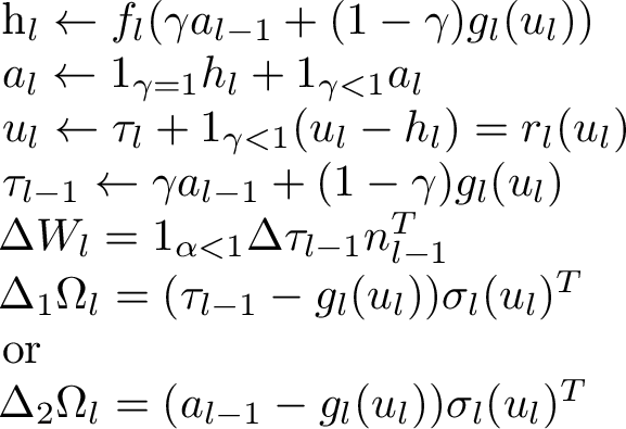where we have considered two variants of the feedback weights update, \(\Delta \tau_l\) is the temporal variation of \(\tau_l\) and \(n_l\) is the normalized value of \(\sigma(a_l)\) (using lateral connections to compute the normalization of the layer \(l\)), i.e., \[\begin{align} n_l = \frac{\sigma(a_l) ||a_L-\tau_L||^2}{||\sigma(a_l)||^2\, ||a_l-\tau_l||^2} \end{align}\] and we have chosen the standard linear+nonlinear parametrization \[\begin{align} f_l(x) &= W_l \sigma(x) \nonumber \\ g_l(y) &= \Omega_l \sigma(y) \end{align}\] with \(\sigma()\) an arbitrary non-linearity (and a bias can be included by having \(\sigma()\) be vector-valued and produce an extra output equal to 1), as in earlier sections of this paper, although it would be straightforward to define other parametrizations for the feedforward and/or feedback paths.

10.2.2 Analysis of the Continuous DTP Equations↩︎

We can verify by inspection of Eqs. 2 and [eq:al] that \(a_l\) acts as a temporary buffer for the activations of the last feedforward phase (obtained while \(\gamma=1\)). Conversely, when \(\gamma=0\), we obtain a purely feedback phase where the encoder \(f_l\) ignores \(a_{l-1}\) and instead is used in an auto-encoder loop which composes \(f_l\) and \(g_l\) and propagates targets.

Let us denote the short-hand \(f'_l\), \(g'_l\) and \(r'_l\) be the Jacobian matrices corresponding to the functions \(f_l\), \(g_l\) and \(r_l\) respectively (at the current value of their arguments).

While the feedforward activations are settling to their value \(a_l\) from their old value (for the previous example), the weight change (if performed) would aim at predicting the new value of \(a_l\) given its previous value, which seems to be a useful feature in a temporal world. However this could also be hindrance (where there is no temporal order) so in Eq. [eq:Wl] we inserted a \(1_{\alpha<1}\) factor to avoid updates until the feedforward phase as settled (note they would be zero once \(a_l\)’s have settled, so long as \(\alpha=1\)). This analysis is also compatible with the idea that \(\tau_l\) becomes a corrected value for \(a_l\), towards which \(a_l\) could move slowly and slightly (not too fast, to make sure the sequence of \(\tau_l\)’s from the top \(\tau_L\) has time to converge).

We note that for \(\gamma\) varying from 1 to 0, \(\tau_{l-1}\) varies linearly from \(a_{l-1}\) to \(g_l(u_l)\), making the update interpolate linearly between minimization of the reconstruction error and helping to hasten the convergence of \(g_l(u_l)\) to make \(g_l(u_l)\) achieve the optimal target propagation \(f_l^{-1}(\tau_l)\).

Hence the two updates are equivalent when \(\gamma=1\), and whereas \(\Delta_1\) goes to 0 when \(\gamma \rightarrow 0\), it is not the case for \(\Delta_2\). The additional pressure \(\Omega_l\) receives under \(\Delta_2\) can thus best be understood by considering \(\gamma \rightarrow 0\). In that case, the feedback units are pushed by \(\Delta_2\) towards \(a_{l-1}\) and not just towards \(f^{-1}(\tau_l)\). This could be seen as a regularizer, especially when there are many inverses: we would prefer to pick among all the inverses ones which are closer to the feedforward activations (i.e. require the least changes in the weights). Another more far-fetched consideration is that in the case where the loss can be interpreted like an energy function and the feedback path as a stochastic generative model (if noise is injected in its computation), then we want that generative path to match the feedforward path, as in the Wake-Sleep algorithm [22].

11 Conclusion and Future Work↩︎

This is only a proposal, with many uncertain avenues left to explore and the need to validate these ideas through simulations and confrontation with biological knowledge (and possibly biological experiments) and machine learning experiments. Many variations on the themes introduced here are possible and will need simulations to disentangle experimentally and understand better. This proposal opens the door to a style of biologically plausible analogues to backprop which is a variant of target propagation while sharing some properties of error propagation schemes (the targets being close to the activations) and can potentially offer optimization advantages compared to SGD with backpropagation, because of the Gauss-Newton approximation implicitly being computed (without having to represent and invert high-dimensional matrices).

One generalization which would be interesting to consider is one in which lower layers would not just try to minimize the output error but also make the inversion easier for upper layers, which could be achieved by extending the kind of feedback loop we analyzed here between consecutive layers to a global feedback look. The general idea is that we are trying to make all latent layers move away from the current feedforward activations in a direction which provides less output error but also a better match between the "prior" top-down information and the "data-driven" bottom-up signal. An important principle exploited in this paper is that we only want to move slightly away from the data-driven inference and towards one which is more globally coherent with other signals (like the target), in order to obtain an update training signal for all the weights. Like in the Wake-Sleep algorithm, we want to make the generative part of the model (the feedback loops) slightly more consistent with the data, and we want to data-driven inference to be slightly more consistent with the global loss.

An interesting longer-term question is whether this principle could also be used to implement a limited analogue to backprop through time. If the brain has a memory of key past events, as well as predictive computations to link them (by a form of association) both forward and backward in time, then all the ingredients are present to achieve credit assignment through time, in a style similar to Sparse Attentive Backtracking [23], [24]. In the spirit of the Consciousness Prior [25], these credit assignment calculations through time may need not be for all the units in some circuit: it would be enough that the forward and backward associations involve only a few relevant high-level semantic variables. The learned back-through-time target propagation could use attention mechanisms to choose aspects of past moments (events) which are relevant and need to be "fixed" to achieve some current targets. Attention could also be used in a top-down fashion when calculating targets, to focus the target change in the most relevant neurons. This is especially relevant when the lower layer for which a target is computed has more neurons than its upper layer.

References↩︎