0.1 Worm-algorithm Monte Carlo

Using a continuous-time worm-algorithm Monte Carlo (WAMC), we simulate a pair of holes in the \(t\)-\(J\) model [1] on a quadratic lattice with \(20 \times 20\) sites and periodic boundary conditions. The WAMC method effectively samples world-line configurations in real-space and imaginary-time by combining the partition function sector and Green’s function sector: In order to go from one partition function world-line configuration to another, one needs to pass through the Green’s function sector [2]. We use two different worms to represent spins and holes. The former is allowed to wind in imaginary-time such that the total spin can vary. Contrary, the hole worm is not, and the number of holes in the partition function sector is therefore kept fixed. All data presented are extracted purely from the sampled partition function configurations. In particular, the kinetic energy presented later in this supplementary information is obtained by counting the kinks involving the hole worm [3].

0.2 Sign problem

When simulating two holes in the \(t\)-\(J\) model using WAMC, there are two types of processes contributing to the fermionic sign problem: exchange of indistinguishable spins and exchange of holes. The former enters first at order \(t^2 J^3\) [4] and the latter at order \(t^4\). When such a process is present in a world-line configuration, the configuration weight \(p\) might turn negative. Hence the name “sign problem”.

In order to account for negative configuration weights in WAMC, we factor the weight \(p\) into its sign \(s = \pm 1\) and magnitude \(|p|\), i.e., \(p = s |p|\). Then, when computing the acceptance ration, \(p\) is exchanged in favor of \(|p|\), and every sampled quantity \(x\) is assigned the sign \(s\) of the world-line configuration. By performing this substitution, the acquired expectation value \(\langle x \rangle'\) is not that of the original fermionic system. However, the latter one is obtained through \(\langle x \rangle = \langle sx \rangle' / \langle s \rangle'\) [5]. This way of circumventing negative configuration weights gives rise to an exponential decrease in signal-to-noise ratio (SNR) and is the hallmark of the sign problem. The decrease of SNR can, in part, be explained by the exponential decay of the denominator \(\langle s \rangle'\) with — in our case — increased values of \(t\beta\) and \(J\beta\). This decay of \(\langle s \rangle'\) is illustrated in Fig. 1.

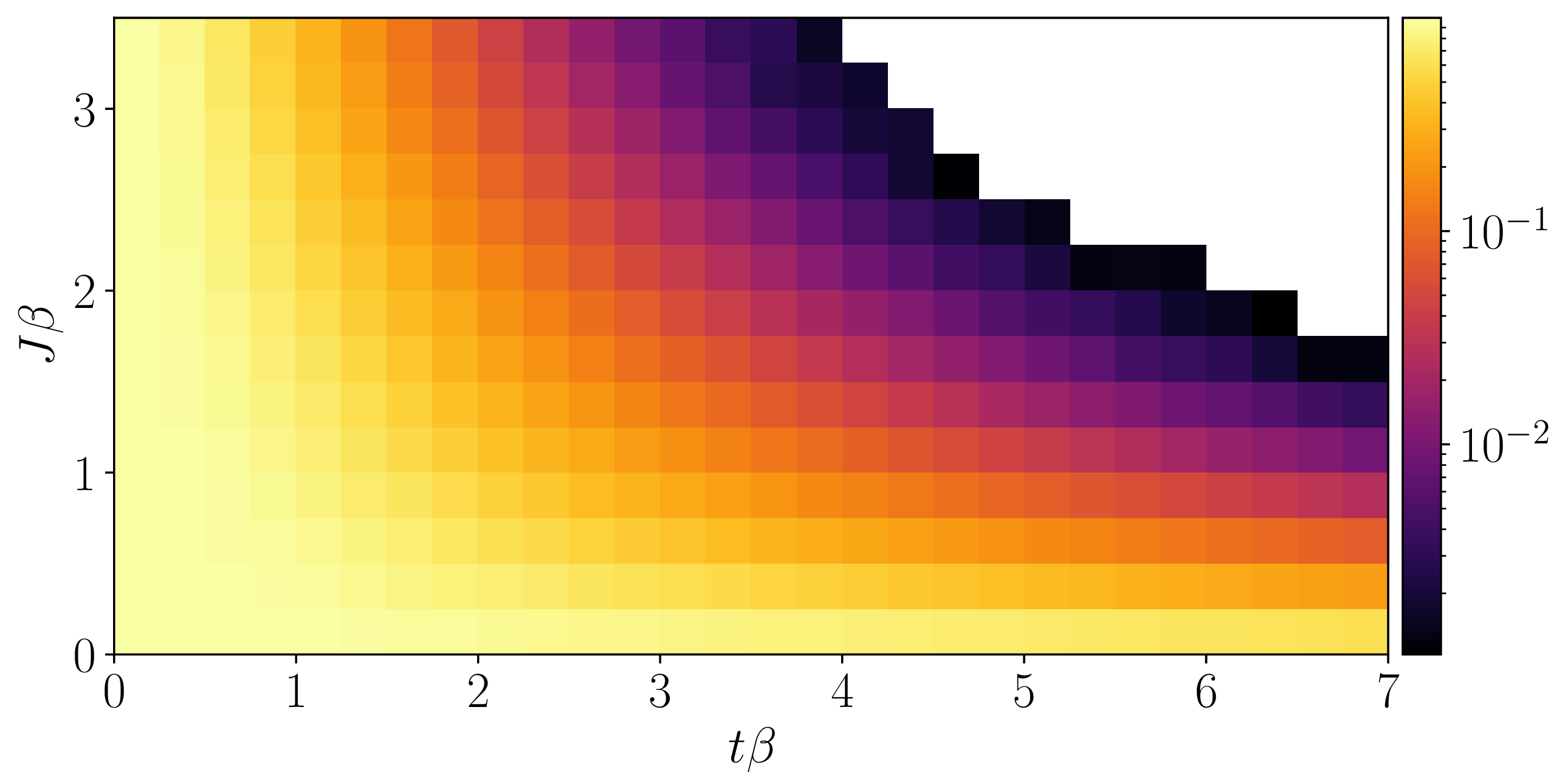
Figure 1: **Average sign.** This plot shows the exponential decay of \(\langle s \rangle'\) with increased values of \(t \beta\) and \(J \beta\). Only values \(\langle s \rangle' > 10^{-3}\) are shown due to an otherwise poor SNR.

0.3 Determining hole-hole attraction

The starting point for determining hole-hole attraction is the hole-hole correlator,

\[\begin{equation}C^\mathrm{h}(\mathbf{s}) = (N-1) \sum \limits_{\mathbf{r}_0} \Big( \big \langle \hat n^\mathrm{h}_{\mathbf{r}_0} \hat n^\mathrm{h}_{\mathbf{r}_0 + \mathbf{s}} \big \rangle - \big \langle \hat n^\mathrm{h}_{\mathbf{r}_0} \big \rangle \big \langle \hat n^\mathrm{h}_{\mathbf{r}_0 + \mathbf{s}} \big \rangle \Big) \,, \label{Ch}\end{equation}\]

which is project onto the separation distance \(s = | \mathbf{s} |\). The resulting radial correlation is then partitioned into two parts: the signal part in which the holes are in the close vicinity of one another \(s < s_\mathrm{bg}\), and the background part where they are further separated \(s \ge s_\mathrm{bg}\). The condition for classifying a parameter point as attractive is that the peak value of the signal partition exceeds the background partition’s peak value — including two standard deviations of uncertainty (noise). This is illustrated in Fig. 2, and the parameter region displaying attraction is shown in Fig. 3.

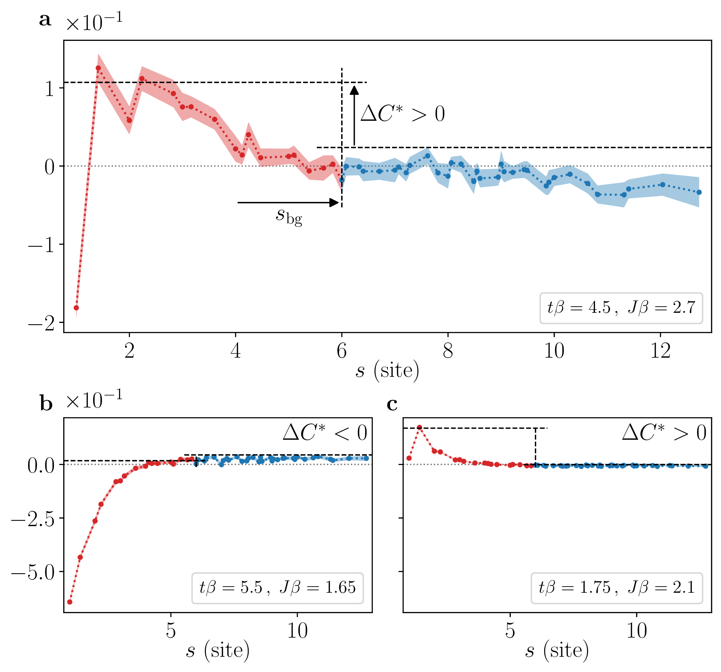
Figure 2: **Determining hole-hole attraction.** Illustrations of how hole-hole attraction is inferred using radially projected hole-hole correlations obtained using WAMC. If the difference \(\Delta C^* = \text{max} (C(s < s_\text{bg})) - \text{max} (C(s \ge s_\text{bg})) - 2 \times \text{noise} > 0\) (a, c), the data is said to indicate attraction, otherwise (b) attraction is deemed to be absent. The partition divider \(s_\text{bg} = 6\) is chosen such that it exceeds separation distances where a peak is observed.

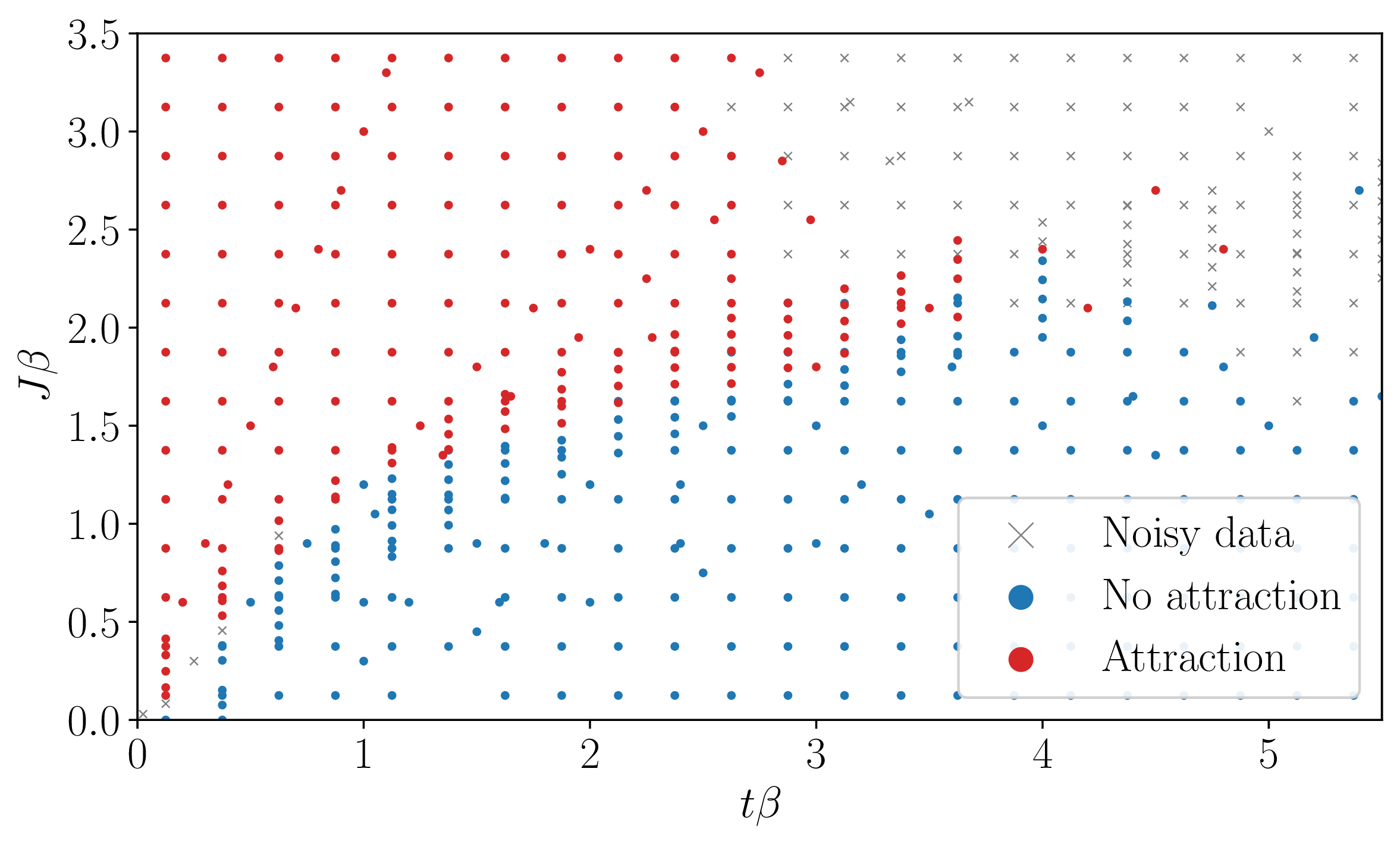
Figure 3: **Attractive parameter region.** Parameter region scanned using WAMC. Red dots indicate observed hole-hole attraction, blue dots signify no observed attraction, and a gray cross mark points deemed to have inadequate SNR. The reason for large parameter values suffering from a poor SNR can be explained by the sign problem (c.f.Fig. 1). On the other hand, the low SNR for small parameter values is caused by a weak signal.

The value of \(s_\mathrm{bg}\) is chosen such that the attractive part of the correlation is not included in the background partition. We choose \(s_\text{bg} = 6\), which exceeds the separation where a peak is observed.

Due to the presence of the fermionic sign problem, the noise grows exponentially with an increased value of \(t \beta\) and \(J \beta\). Data at these parameter values, therefore, suffer from a poor SNR. Data at small values of \(t \beta\) and \(J \beta\) also have a low SNR, but here the reason being a weak signal. To filter out noisy data, the SNR is defined as \((C_\mathrm{max} - C_\mathrm{min})^2 / \langle n^2 \rangle\), i.e., the ratio of squared signal amplitude to mean square noise. A data point is deemed too noisy and ignored if \(\text{SNR} < 200\).

To reduce noise, the outer edges of the background correlation, where \(s_x, s_y = 10\) (we performed simulations on systems with \(20 \times 20\) lattice sites), are omitted. These omitted correlation values merely carry half, or even a quarter, of the statistical weight compared to other background values. The SNR of the remaining correlator is, therefore, improved.

To further improve SNR, we ultimately performed large-scale simulations, amounting to several million core-hours. The number of sampled world-line configurations for different values of \(t\beta\) and \(J\beta\) is shown in Fig. 4.

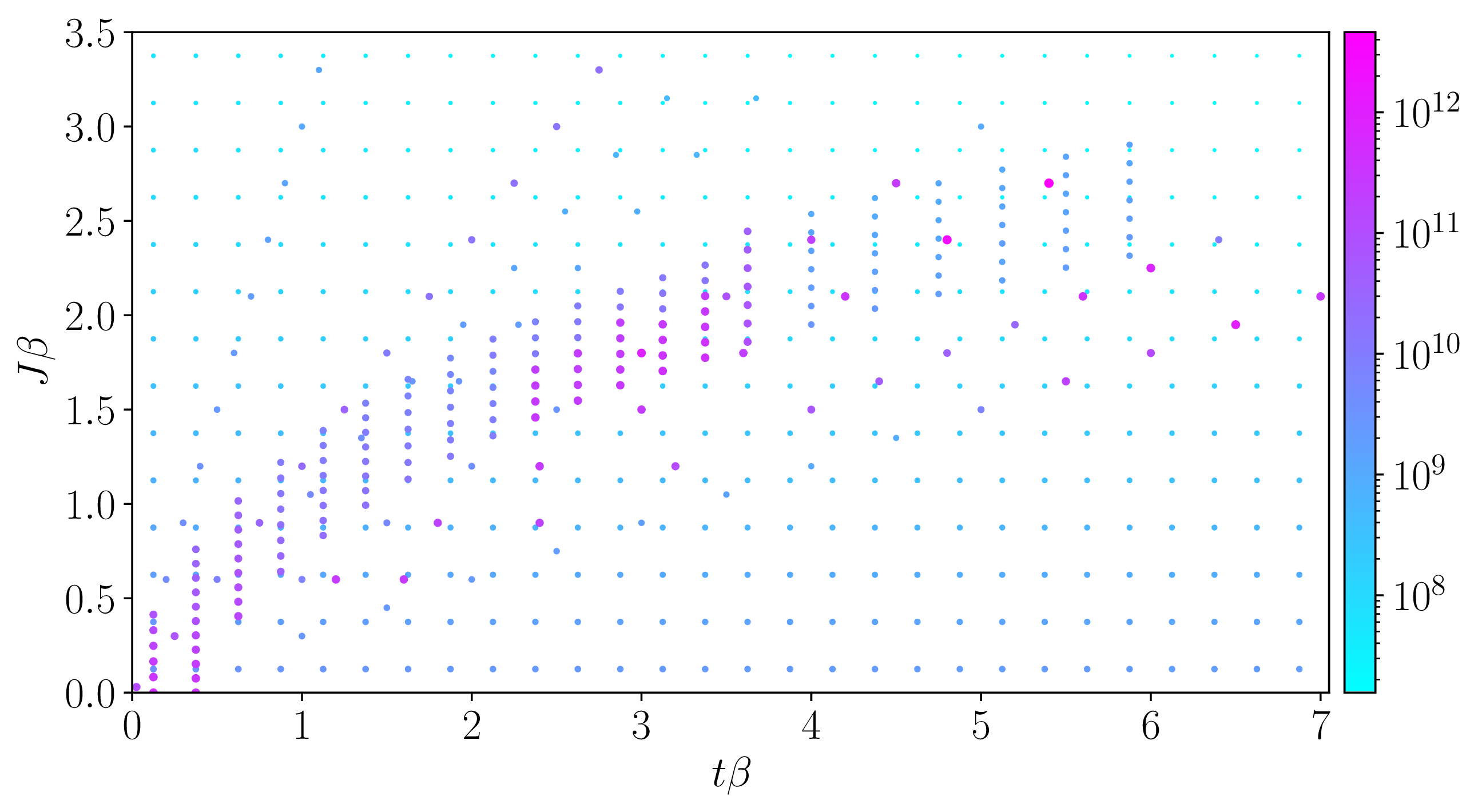
Figure 4: **Extent of simulation.** This figure illustrates the number of sampled world-line configurations in the partition function sector for different values of \(t \beta\) and \(J \beta\). The combined total simulation time amounts to several million core-hours.

0.4 Additional hole-hole correlation data

In Fig.5, 6, we present additional data of the hole-hole correlator defined in Eq. \(\ref{Ch}\).

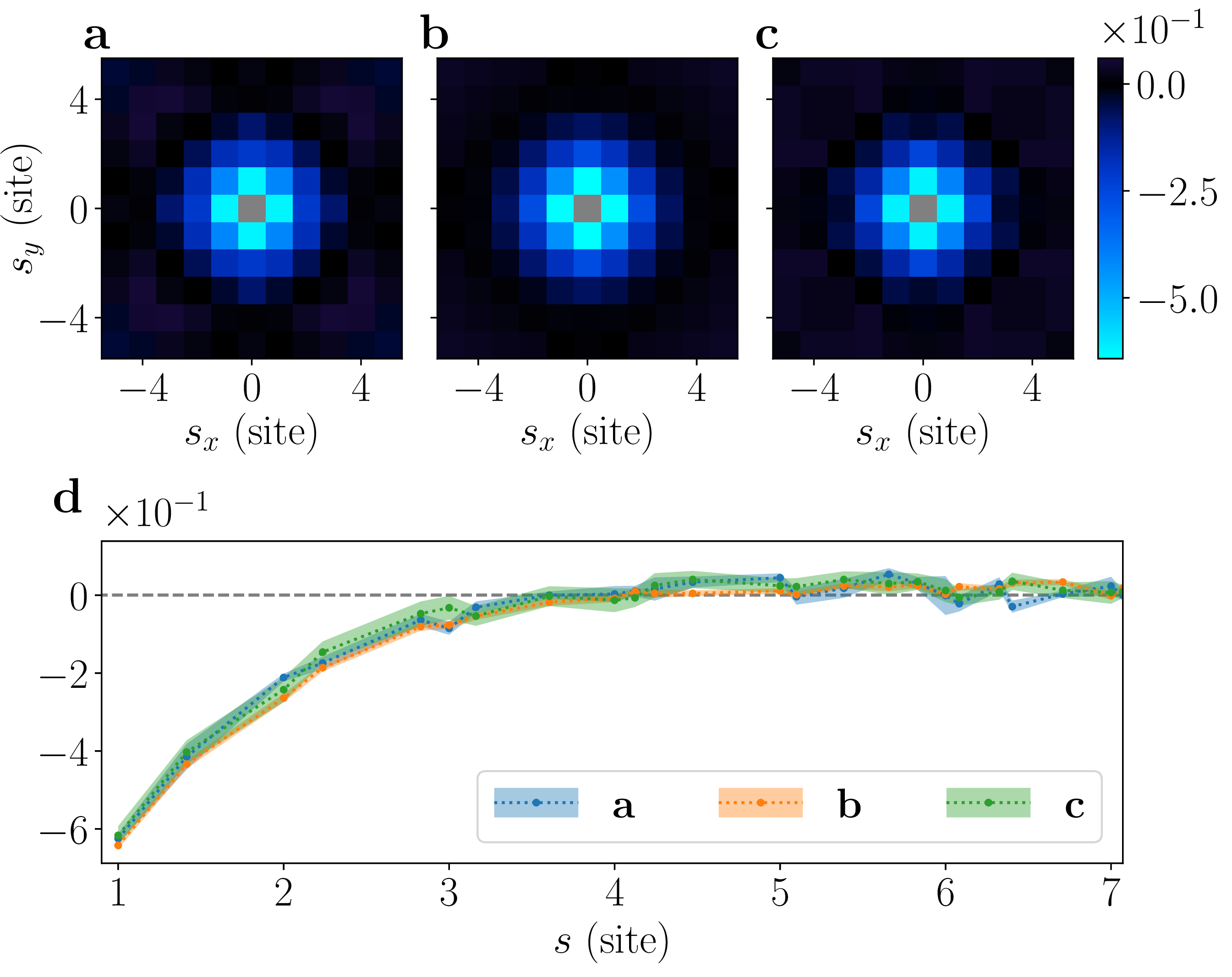
Figure 5: **Hole-hole correlations.** (a-c) show contour plots of the correlator \(C^\mathrm{h}(\mathbf{s})\) for the case \(t/J = 10/3\) and \(\beta J = 1.35,\;1.65,\;1.95\), respectively. The radial components of these are given in (d). No attraction is found for these parameter values.

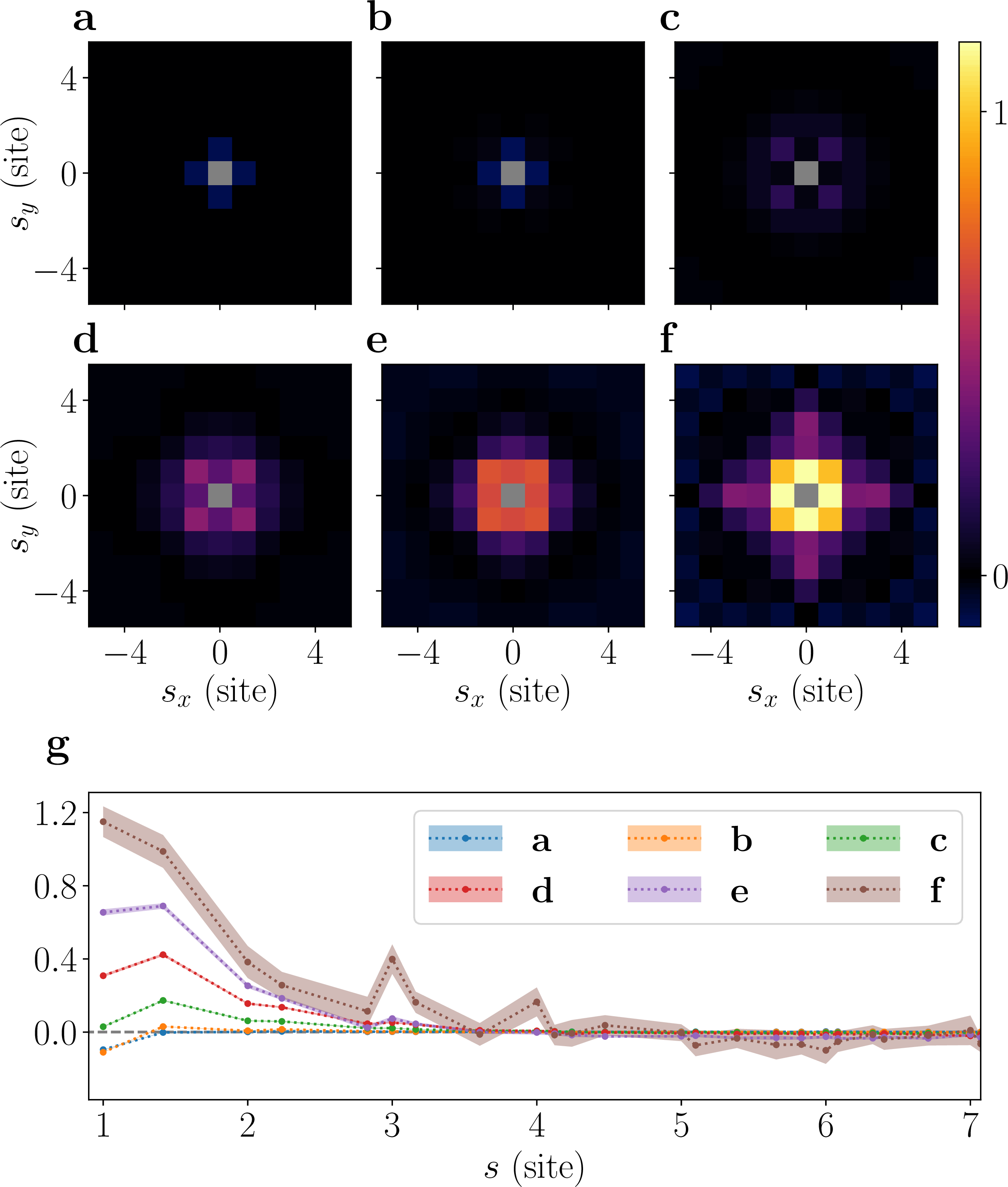
Figure 6: **Hole-hole correlations.** (a-f) show contour plots of the correlator \(C^\mathrm{h}(\mathbf{s})\) for the case \(t/J = 5/6\) and \(\beta J = 0.90,\;1.50,\;2.10,\;2.70,\;3.30,\;3.90\), respectively. The radial components of these are given in (g). Attraction is present for all of these parameter values.

0.5 Additional spin-spin correlation data

In Fig.7-9, we present additional data of the spin-spin correlator, defined by

\[\begin{equation} C^\mathrm{s}_{\mathbf{|d|}, \mathbf{s}}(\mathbf{r}) = 4 \frac{ \sum \limits_{\mathbf{r}_0} \big \langle \hat n^\mathrm{h}_{\mathbf{r}_0} \hat n^\mathrm{h}_{\mathbf{r}_0 + \mathbf{s}} \hat S^z_{\mathbf{r}_0 + \mathbf{r} - \mathbf{d}/2} \hat S^z_{\mathbf{r}_0 + \mathbf{r} + \mathbf{d}/2} \big \rangle }{ \sum \limits_{\mathbf{r}_0} \big \langle \hat n^\mathrm{h}_{\mathbf{r}_0} \hat n^\mathrm{h}_{\mathbf{r}_0 + \mathbf{s}} \big \rangle } \,.\label{eq:spin-corr}\end{equation}\]

Further examples are given as animations [6].

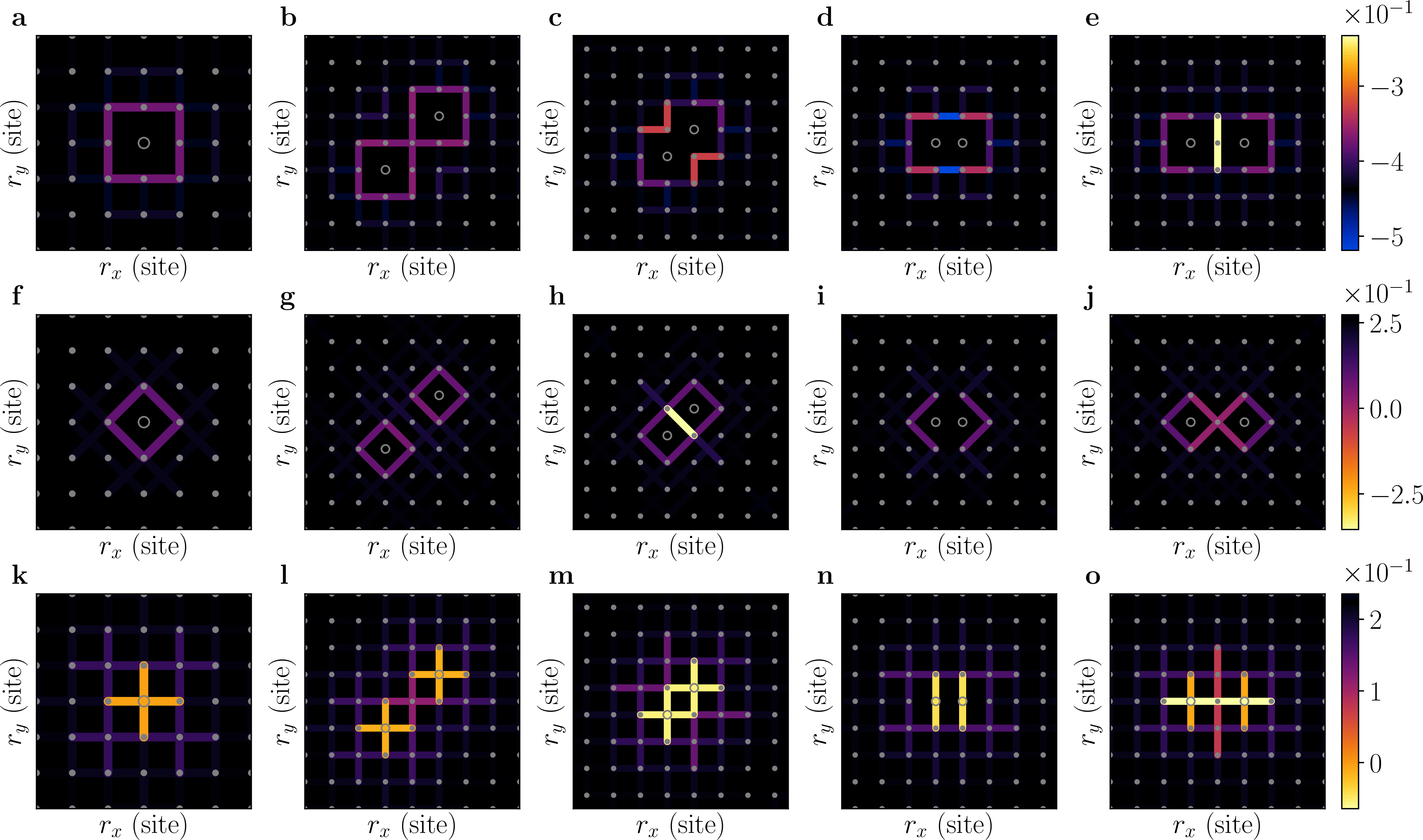
Figure 7: **Spin correlations \(C^\mathrm{s}_{|\mathbf d|, \mathbf s}(\mathbf r)\).** Left column depicts a single hole, while the remaining columns depict two dopants located in the close vicinity of one another. The top row (a - e) gives \(C^\mathrm{s}_{|\mathbf d|=1, \mathbf s}(\mathbf r)\), middle row (f - j) gives \(C^\mathrm{s}_{|\mathbf d|=\sqrt{2}, \mathbf s}(\mathbf r)\), and bottom row (k - o) gives \(C^\mathrm{s}_{|\mathbf d|=2, \mathbf s}(\mathbf r)\). Model parameters are \(t \beta = 2.75\) and \(J \beta = 3.3\).

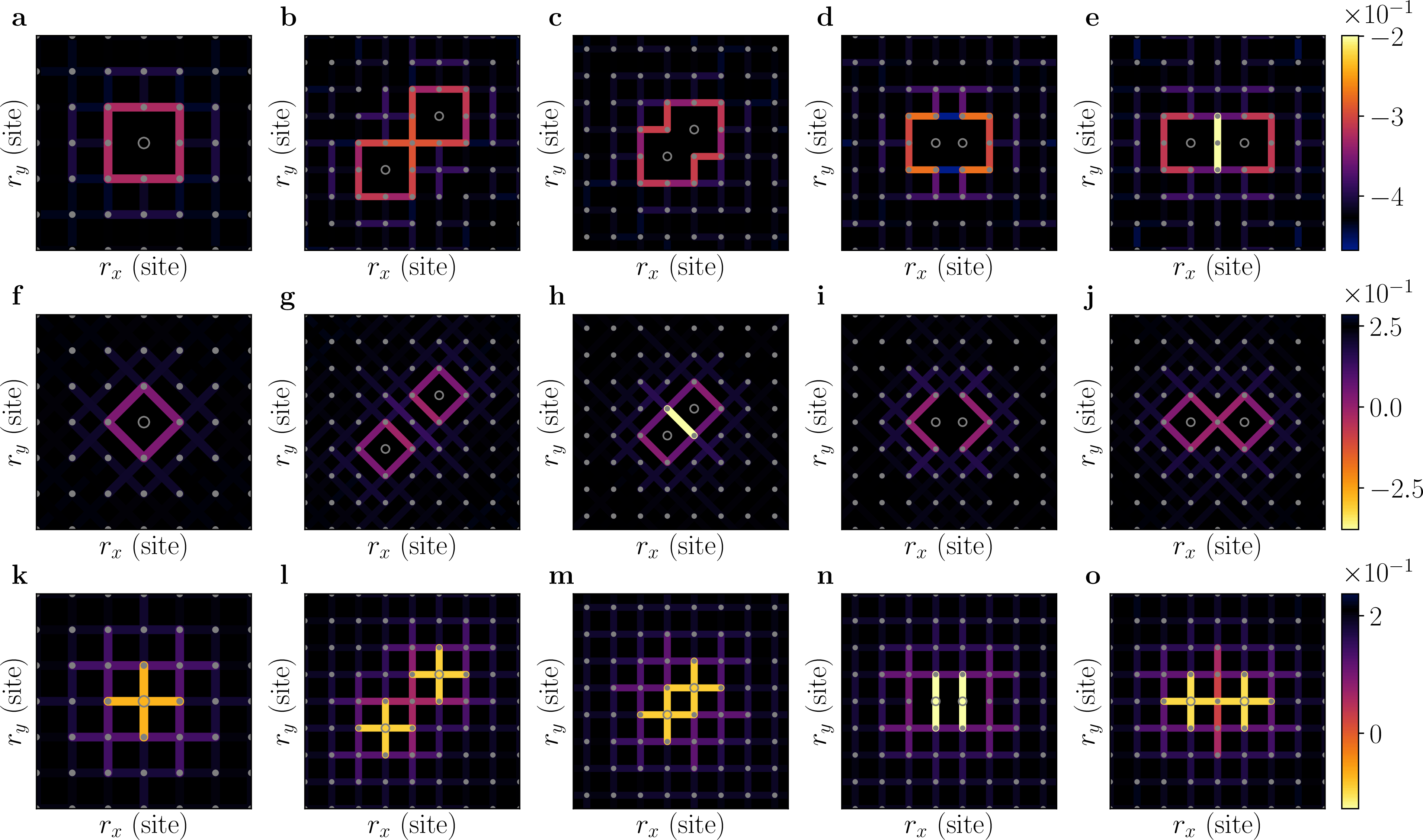
Figure 8: **Spin correlations \(C^\mathrm{s}_{|\mathbf d|, \mathbf s}(\mathbf r)\).** Left column depicts a single hole, while the remaining columns depict two dopants located in the close vicinity of one another. The top row (a - e) gives \(C^\mathrm{s}_{|\mathbf d|=1, \mathbf s}(\mathbf r)\), middle row (f - j) gives \(C^\mathrm{s}_{|\mathbf d|=\sqrt{2}, \mathbf s}(\mathbf r)\), and bottom row (k - o) gives \(C^\mathrm{s}_{|\mathbf d|=2, \mathbf s}(\mathbf r)\). Model parameters are \(t \beta = 4.5\) and \(J \beta = 2.7\).

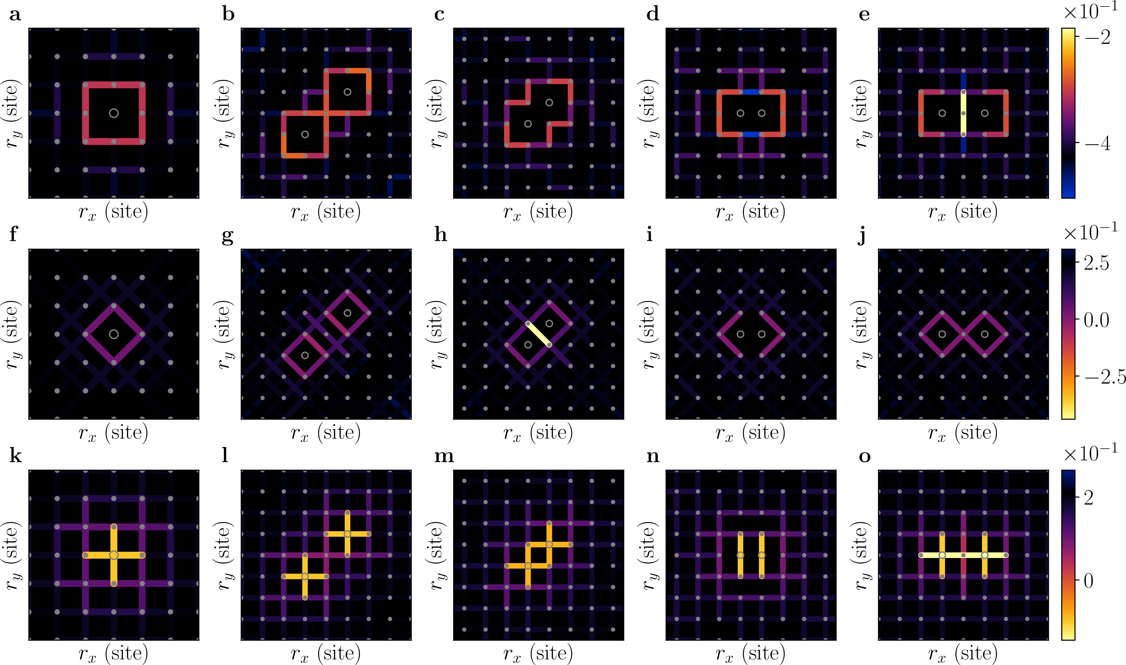
Figure 9: **Spin correlations \(C^\mathrm{s}_{|\mathbf d|, \mathbf s}(\mathbf r)\).** Left column depicts a single hole, while the remaining columns depict two dopants located in the close vicinity of one another. The top row (a - e) gives \(C^\mathrm{s}_{|\mathbf d|=1, \mathbf s}(\mathbf r)\), middle row (f - j) gives \(C^\mathrm{s}_{|\mathbf d|=\sqrt{2}, \mathbf s}(\mathbf r)\), and bottom row (k - o) gives \(C^\mathrm{s}_{|\mathbf d|=2, \mathbf s}(\mathbf r)\). Model parameters are \(t \beta = 5.4\) and \(J \beta = 2.7\).

0.6 Exact Diagonalization

In order to verify the accuracy of WAMC, it is been benchmarked against exact diagonalization (ED) [7] on a system of \(4 \times 4\) lattice sites with periodic boundaries, containing a single carrier. In Fig. 10 we present average kinetic energy results, which indicate a perfect agreement between the unbiased WAMC and exact ED method.

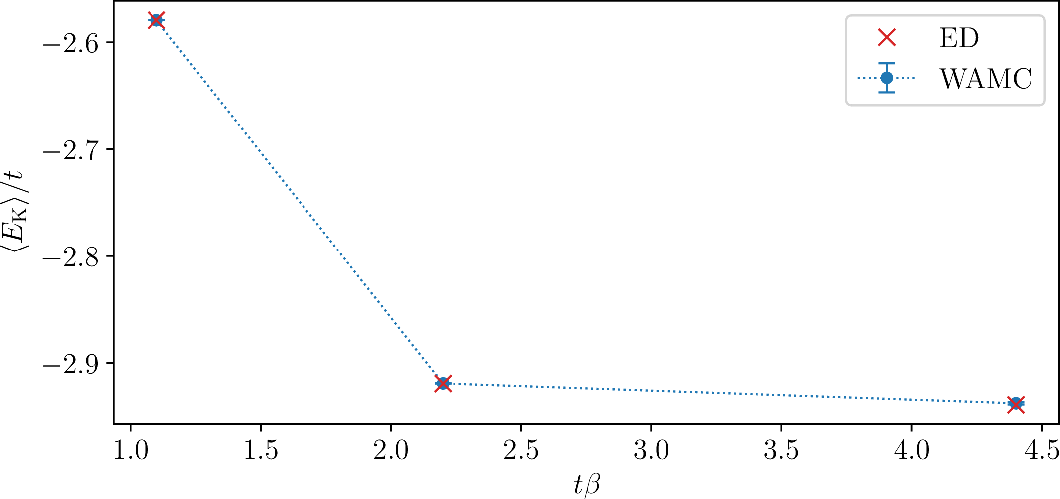
Figure 10: **Kinetic energy.** A single carrier’s average kinetic energy, as a function of temperature, in a system of \(4 \times 4\) lattice sites with periodic boundary conditions. The ratio of hopping strength to super-exchange strength is \(t/J = 10/3\). While error bars are given for the WAMC data, they are smaller than the marker size. The data indicate a perfect agreement between WAMC and ED.

References

[1] J. Spałek, “T-j model then and now: A personal perspective from the pioneering times,” Acta Physica Polonica A, vol. 111, pp. 409–424, Apr. 2007, doi: 10.12693/APhysPolA.111.409.

[2] N. V. Prokof’ev, B. V. Svistunov, and I. S. Tupitsyn, “Exact, complete, and universal continuous-time worldline monte carlo approach to the statistics of discrete quantum systems,” Journal of Experimental and Theoretical Physics, vol. 87, no. 2, pp. 310–321, Aug. 1998, doi: 10.1134/1.558661.

[3] K. Sellin, “Structure formation, phase transitions and drag interactions in multicomponent superconductors and superfluids,” PhD thesis, KTH, Statistical Physics; KTH, Statistical Physics, 2018.

[4] A. S. Mishchenko, N. V. Prokof’ev, and B. V. Svistunov, “Single-hole spectral function and spin-charge separation in the \(t\ensuremath{-}J\) model,” Phys. Rev. B, vol. 64, no. 3, p. 033101, Jun. 2001, doi: 10.1103/PhysRevB.64.033101.

[5] M. Troyer and U.-J. Wiese, “Computational complexity and fundamental limitations to fermionic quantum monte carlo simulations,” Phys. Rev. Lett., vol. 94, no. 17, p. 170201, May 2005, doi: 10.1103/PhysRevLett.94.170201.

[6] E. Blomquist, “Hole-hole and spin-spin correlations in the t-j model,” 20, 2020. https://www.youtube.com/watch?v=9f-0qDY1UTU.

[7] A. W. Sandvik, “Computational studies of quantum spin systems,” AIP Conference Proceedings, vol. 1297, no. 1, pp. 135–338, 2010, doi: 10.1063/1.3518900.

Supplementary Information

Subjects

Updated on Academus