Efficient Proximal Mapping of the 1-path-norm of Shallow Networks
July 02, 2020
Abstract
We demonstrate two new important properties of the 1-path-norm of shallow neural networks. First, despite its non-smoothness and non-convexity it allows a closed form proximal operator which can be efficiently computed, allowing the use of stochastic proximal-gradient-type methods for regularized empirical risk minimization. Second, when the activation functions is differentiable, it provides an upper bound on the Lipschitz constant of the network. Such bound is tighter than the trivial layer-wise product of Lipschitz constants, motivating its use for training networks robust to adversarial perturbations. In practical experiments we illustrate the advantages of using the proximal mapping and we compare the robustness-accuracy trade-off induced by the 1-path-norm, L1-norm and layer-wise constraints on the Lipschitz constant (Parseval networks).
1 Introduction↩︎
Neural networks are the backbone of contemporary applications in machine learning and related fields, having huge influence and significance both in theory and practice. Among the most important and desirable attributes of a trained network are robustness and sparsity. Robustness, is often defined as stability to adversarial perturbations, such as in supervised classification methods. The apparent brittleness of neural networks to adversarial attacks in this context has been considered in the literature for some time, see e.g., [1]–[3] and references therein.
A fundamental question in this regard is how to measure robustness, or more importantly, how to encourage it. One prominent approach supported by theory and practice [4], [5], is to use the Lipschitz constant of the network function to quantize robustness, and regularization to encourage it.
This approach is also supported theoretically with generalization bounds in terms of the layer-wise product of spectral norms [6], [7], which particularly upper-bounds the Lipschitz constant. However, a recent empirical study [8] has found in practice a negative correlation of this measure with generalization. This casts doubts on its usefulness and signals the fact that it is a rather loose upper bound for the Lipschitz constant [9].
Current methods that compute upper bounds on the Lipschitz constant of neural networks can be roughly classified into two classes: (i) the class of product bounds, comprising all upper bounds obtained by the multiplication of layer-wise matrix norms; and, (ii) the class of convex-optimization-based bounds, which addresses the network as a whole entity [4], [9], [10].
A trade-off between computational complexity and quality of the upper bound seems apparent. An ideal bound would achieve a balance between both properties: it should provide a good estimate of the constant while being fast and easy to minimize with iterative first-order algorithms.
Recently, the path-norm of the network [11] has emerged as a complexity measure that is highly-correlated with generalization [8]. Thus, its use as a regularizer holds an increasing interest for researchers in the field.
Despite existing generalization bounds [11], our understanding of the optimization aspects of the path-norm-regularized objective is lacking. [8] refrained from using automatic-differentiation methods in this case because, as they argue, the optimization could fail, thus providing no conclusion about its qualities.
It is then natural to ask: how do we properly optimize the path-norm-regularized objective with theoretical guarantees? What conclusions can we draw about the robustness and sparsity of path-norm-regularized networks? We focus on the 1-path-norm and provide partial answers to those questions, further advancing our understanding of this measure. Let us summarize our main contributions:
Optimization. We show a striking property of the 1-path-norm, that makes it a strong candidate for explicit regularization: despite its non-convexity, it admits an efficient proximal mapping (Algorithm 3). This allows the use of proximal-gradient type methods which are, as of now, the only first-order optimization algorithms to provide guarantees of convergence for composite non-smooth and non-convex problems [12].
Indeed, automatic differentiation modules of popular deep learning frameworks like PyTorch [13] or TensorFlow [14] may not compute the correct gradient for compositions of non-smooth functions, at points where these are differentiable [15], [16]. Our proposed optimization algorithm avoids such issue altogether by using differentiable activation functions like ELU [17] and our novel proximal mapping of the 1-path-norm.
Upper bounds. We show that the 1-path-norm [11] achieves a sweet spot in the computation-quality trade-off observed among upper bounds of the Lipschitz constant: it has a simple closed formula in terms of the weights of the network, and it provides an upper bound on the \((\ell_\infty, \ell_1)\)-Lipschitz constant (cf., 1), which is always better than the product bound.
Sparsity. Neural network regularization schemes promoting sparsity in a principled way are of great interest in the growing field of compression in Deep Learning [18], [19].
Our analysis provides a formula (cf. Lemma 4) for choosing the strength of the regularization, which enforces a desired bound on the sparsity level of the iterates generated by the proximal gradient method. This is a suprising, yet intuitive, result, as the sparsity-inducing properties of non-smooth regularizers have been observed before in convex optimization and signal processing literature, see e.g., [20], [21].
Experiments. In 7, we present numerical evidence that our approach (i) converges faster and to lower values of the objective function, compared to plain SGD; (ii) generates sparse iterates; and, (iii) the magnitude of the regularization parameter of the 1-path-norm allows a better accuracy-robustness trade-off than the common \(\ell_1\) regularization or constraints on layer-wise matrix norms.
2 Problem Setup↩︎
We consider the so-called shallow neural networks with \(n\) hidden neurons and \(p\) outputs \(h:\mathbb{R}^m \rightarrow \mathbb{R}^p\) given by \[\label{eq:nn} h_{V,W}(x) = V^T \sigma(Wx),\tag{1}\] where \(V \in \mathbb{R}^{n \times p}, W\in \mathbb{R}^{n\times m}\) and \(\sigma:\mathbb{R} \rightarrow \mathbb{R}\) is some differentiable activation function with derivative globally bounded between zero and one. This condition is satisfied, for example, by the ELU or softplus activation functions. To control the robustness of the network to perturbations of its input \(x\), we want to regularize training using its Lipschitz constant as a function of the weights \(V\) and \(W\).
To properly define this constant, we utilize the \(\ell_\infty\)-norm for the input space, and the \(\ell_1\)-norm for the output space. Exact computation of such constant is a hard task. A simple and easily computable upper bound can be derived by the product of the layer-wise Lipschitz constants, however, it can be quite loose.
We derive an improved upper bound which is still easy to compute. In the following, we denote with \(\|W\|_\infty\) the operator norm of a matrix \(W\) with respect to the \(\ell_\infty\) norm for both input and output space; it is equal to the maximum \(\ell_1\)-norm of its rows. We denote with \(\|V\|_{\infty, 1}\) the operator norm of the matrix \(V\) with respect to the \(\ell_\infty\) norm in input space and \(\ell_1\)-norm in output space; it is equal to the sum of the \(\ell_1\) norm of its columns.
Theorem 1. Let \(h_{V, W}(x)=V^T \sigma(Wx)\) be a network such that the derivative of the activation \(\sigma\) is globally bounded between zero and one. Choose the \(\ell_\infty\)- and \(\ell_1\)-norm for input and output space, respectively. The Lipschitz constant of the network, denoted by \(L_{V,W}\) is bounded as follows: \[\label{eq:upper95bound} L_{V, W} \leq \sum_{i=1}^n\sum_{j=1}^m\sum_{k=1}^p |W_{ij}V_{ik}| \leq \|V^T\|_{\infty, 1} \|W\|_\infty\qquad{(1)}\]
The proof is provided in appendix 9. The term in the middle of inequality ?? belongs to the family of path-norms, introduced in [11]. Throughout, we refer to it as the 1-path-norm.
Notice that although the path-norm and layer wise product bounds can be equal, this only happens in the following worst case: For the weight matrix in the first layer, the 1-norms of every row are equal. Thus, in practice the bounds can differ drastically.
Remark 1. In practice, one might want to regularize each ouput of the network in a different way according to some weighting scheme [4]. Precisely, the 1-path-norm of the network is equal to the sum (with equal weight) of the 1-path-norm of each output. A weighted version of the 1-path-norm can be defined to account for such a weighting scheme. All our results can be adapted to this scenerio, with minor changes.
We now turn to the task of minimizing an empirical risk functional regularized by the improved upper bound on the Lipschitz constant given in (?? ): \[\label{eq:objective} \min_{V,W} \mathbb{E}_{(x, y)}[\ell(h_{V, W}(x), y)] + \lambda \sum_{i=1}^n\sum_{j=1}^m\sum_{k=1}^p |W_{ij}V_{ik}|\tag{2}\] The objective function in problem 2 is composed of an expectation of a nonconvex smooth loss, and a nonconvex nonsmooth regularizer, meaning that it is essentially a composite problem (cf. [22]). That is, the objective function 2 can be cast as use these notation hereafter) \[\label{eq:objective95fn} \min_{V, W} \mathcal{F} (V, W) \equiv f(V, W) + \lambda g(V, W),\tag{3}\] where \(f\) is a nonconvex continuously differentiable function, and \(g(V, W)= \sum_{i=1}^n\sum_{j=1}^m\sum_{k=1}^p |W_{ij}V_{ik}|\) is a continuous, nonconvex, nonsmooth, function. We assume that the objective function is bounded below, i.e., \(\displaystyle\mathop{\rm inf}\mathcal{F} :=\mathcal{F}_*>0\).
A natural choice for a scheme to obtain critical points for (3 ) is the proximal-gradient framework. However, for a nonconvex \(g\), solving the proximal gradient problem is a hard problem in general. In Section 4 we develop a method that computes the proximal gradient with respect to \(g\) efficiently.
To streamline our approach and techniques in a compact and user-friendly manner, we will illustrate the majority of our results and proofs via the particular single-output scenario in which \(h\) and \(g\) are reduced to \[h_{v, W}(x) = v^T \sigma(Wx), \;g (v,W) \equiv \lambda \| \mathop{\mathrm{vec}}(\mathop{\mathrm{Diag}}(v)W) \|_1.\] The multi-output case follows from the same techniques and insights, however, requires more tedious computations and arguments, on which we elaborate in Section 5, and detail in the appendix.
3 The Prox-Grad Method↩︎
Assume that \(f\) has a Lipschitz continuous gradient with Lipschitz constant \(L>0\), that is \[\| \nabla f(z) - \nabla f(u) \| \leq L \| z - u\|, \qquad \forall z,u \in\mathbb{R}^n.\] The prox-grad method is described by Algorithm 1; since \(g\) is nonconvex, the prox in 4 can be a set of solutions.

Theoretical guarantees for the prox-grad method with respect to a nonconvex regularizer were established by [12] (for a more general prox-grad type scheme).
Theorem 2 (Convergence guarantees). Let \(\{z^k\}_{k\geq 0}\) be a sequence generated by Algorithm 1 with \(\{\eta^k\}_{k\geq 0} \subseteq (0,1/L)\). Then
Any accumulation point of \(\{z^k\}_{k\geq 0}\) is a critical point of 3 .
If \(f\) satisfies the Kurdyka-Lojasiewicz (KL) property, then \(\{z^k\}_{k\geq 0}\) converges to a critical point.
Suppose that \(\eta_k\) is chosen such that there exists \(c > 0\) such that \(\sum_{k=0}^{K}\frac{1}{\eta_k} \geq c K\) for any \(K\geq 0\). Then \[\min_{k=0,\dots,K} \|z^{k+1} - z^k \|_2 \leq \sqrt{\frac{2(\mathcal{F}(z^0) - \mathcal{F}_*)}{(c-L)K}}.\]
Proof. See Section 10 in the appendix. ◻
Remark 2 (On KL related convergence rate). A convergence rate result under the KL property can be derived with respect to the desingularizing function; see [12] for additional details.
Remark 3 (On the stochastic prox-grad method). The literature does not provide any theoretical guarantees for a prox-grad type method that uses stochastic gradients (i.e., replacing \(G^k\) with an approximation of \(\nabla f(z^k)\)) under our setting. Recently, [23] studied stochastic prox-grad methods, however, their results rely on the assumption that the regularizer is Lipschitz continuous, which is not satisfied by our robust-sparsity regularizer.
4 Computing the Proximal Mapping↩︎
Throughout this section we assume the single-output setting. The path-norm regularizer we propose is a nonconvex nonsmooth function, suggesting that the prox-grad scheme in Algorithm 1 is intractable.
In this section we will not only prove that in fact it is tractable in the single output case, but that it can also be implemented efficiently with complexity of \(O(m\log(m))\); we prove the stated in detail in Section 11, and provide here a concise version.
Denote the given pair \((x, Y)\) by \(z\). The proximal mapping with respect to \(\lambda g\) at \(z\) is defined as \[\label{eq:proximal} \mathop{\mathrm{prox}}_{\lambda g}(z) = \displaystyle\mathop{\rm argmin}_{u} \lambda g(u) + \frac{1}{2} \|{\mathop{\mathrm{vec}}(u - z)}\|_2^2.\tag{4}\] By the choice of \(g\), the objective function in 4 is coercive and lower bounded, implying that there exists an optimal solution (cf. [24]).
Remark 4. The derivations in this section can be easily adapted and used with adaptive gradient methods* like Adagrad [25], by a careful handling of the per-coordinate scaling coefficients.*
Lemma 1 (Well-posedness of 4 ). For any \(\lambda\geq 0\) and any \((u,z)\), the problem 4 has a global optimal solution.
Additionally, we have that 4 is separable with respect to the \(i\)-th entry of the vector \(v\) and the \(i\)-th row of the matrix \(W\), meaning that problem 4 can be solved in a distributed manner by applying the same solution procedure coordinate-wise for \(v\) and row-wise for \(W\). In light of this, let us consider the \(i\)-th row related problem \[\label{eq:7b} \min_{v, w\in\mathbb{R}\times\mathbb{R}^m} \frac{1}{2} (v-x)^2 + \frac{1}{2} \sum_{j=1}^m (w_j - y_j)^2 + \lambda |v| \sum_{j=1}^m |w_j|.\tag{5}\] The signs of the elements of the decision variables in (5 ) are determined by the signs of \((x, y)\), and consequently, the problem in (5 ) is equivalent to \[\label{eq:cw95prox95prob} \min_{v, w\in\mathbb{R}_+\times\mathbb{R}_+^m} \frac{1}{2} (v-|x|)^2 + \frac{1}{2} \sum_{j=1}^m (w_j - |y_j|)^2 + \lambda v \sum_{j=1}^m w_j.\tag{6}\]
Lemma 2. Let \((v^*, w^*)\in\mathbb{R}_+\times\mathbb{R}_+^n\) be an optimal solution of 6 . Then \((sign(x) \cdot v^*, sign(y) \circ w^*)\) is an optimal solution of problem 5 .
Denote \[h_\lambda(v,w;x,y)= \frac{1}{2} (v-|x|)^2 + \frac{1}{2} \sum_{j=1}^m (w_j - |y_j|)^2 + \lambda v \sum_{j=1}^m w_j.\] Although \(h_\lambda\) is nonconvex, we will show that a global optimum to 6 can be obtained efficiently by utilizing several tools, the first being the first-order optimality conditions of 6 (cf. [24]) given below.
Lemma 3 (Stationarity conditions). Let \((v^*, w^*)\in \mathbb{R}_+\times\mathbb{R}_+^m\) be an optimal solution of 6 for a given \((x,y)\in \mathbb{R}\times\mathbb{R}^m\). Then \[\begin{align} w_j^* &= \max \left\lbrace 0, |y_j| - \lambda v^* \right\rbrace \;\text{ for any } j=1,2,\ldots,m,\\ v^* &= \max\left\lbrace 0, |x| - \lambda \sum_{j=1}^{m} w^*_j \right\rbrace. \end{align}\]
A key insight following Lemma 3 is that: the elements of any solution to 6 , satisfy a monotonic relation in magnitude, correlated with the magnitude of the elements of \(y\); this is formulated by the next corollary.
Corollary 1. Let \((v^*, w^*)\in \mathbb{R}_+\times\mathbb{R}_+^m\) be an optimal solution of 6 for a given \((x,y)\in \mathbb{R}\times\mathbb{R}^m\). Then
The vector \(w^*\) satisfies that for any \(j,l\in\{1,2,\ldots,m \}\) it holds that \(w^*_j \geq w^*_l\) only if \(|y_j| \geq |y_l|\).
Let \(\bar{y}\) be the sorted vector of \(y\) in descending magnitude order. Suppose that \(v^* > 0\) and let \(s= | \{ j : sw^*_j > 0 \} |\). Then, \[\label{eq:2b} v^* = \dfrac{1}{1-s \lambda^2}\left(|x| - \lambda\sum_{j=1}^s|\bar{y}_j|\right),\qquad{(2)}\] where we use the convention that \(\sum_{j=1}^0|\bar{y}_j| = 0\).
Proof. The first part follows trivially from the stationarity conditions on \(w^*\) given in Lemma 3.
From the first part and the conditions in Lemma 3 we have that \(\sum_{j=1}^{m} w^*_j = \sum_{j=1}^s|\bar{y}_j| - \lambda s v^*\). Plugging the latter to the stationarity condition on \(v^*\) (given in Lemma 3) then implies the required. ◻
Remark 5. Corollary 1 implies that the solution vector \(w^*\) is ordered in the same way as \(|y|\). Thus, the \(s\) non-zero entries of \(w^*\) are precisely the ones corresponding with the \(s\) largest entries of \(|y|\).
Without loss of generality, we assume hereafter that the input \(y\) is already sorted in decreasing order, such that the \(s\) non-zero entries of \(w^*\) are always the first \(s\) entries.
To supplement the results above, we now show that we can actually upper-bound the sparsity level of the prox-grad output by adjusting the value of \(\lambda\).
Lemma 4 (Sparsity bound). Let \((v^*, w^*)\in \mathbb{R}_+\times\mathbb{R}_+^m\) be an optimal solution of 6 for a given \((x,y)\in \mathbb{R}\times\mathbb{R}^m\). Suppose that \(v^* > 0\) (i.e., non-trivial),1 and denote \(S = \{ j : w^*_j > 0 \}\). Then \(|S|\leq \lambda^{-2}\).
Proof. Since \((v^*, w^*)\) is an optimal solution of 6 and the objective function in 6 is twice continuously differentiable, \((v^*, w^*)\) satisfies the second order necessary optimality conditions [26]. That is, for any \(d\in\mathbb{R}\times\mathbb{R}^m\) satisfying that \((v^*, w^*)+d \in \mathbb{R}_+\times\mathbb{R}_+^m\) and \(d^T \nabla h_\lambda(v^*, w^*;x,y) = 0\) it holds that \[d^T \nabla^2 h_\lambda(v^*, w^*;x,y)d = d^T \left( \begin{array}{ccccc} 1 & \lambda &\cdots &\lambda \\ \lambda& 1& 0& 0 \\ \vdots& 0& \ddots&0 \\ \lambda& 0 & 0& 1 \end{array} \right) d \geq 0,\] where the first row/column corresponds to \(v\) and the others correspond to \(w\). Noting that for any \(j\in S\) it holds that \(\frac{\partial h_\lambda}{\partial w_j} (v^*, w^*;x,y) = 0\), we have that the submatrix of \(\nabla^2 h_\lambda(v^*, w^*;x,y)\) containing the rows and columns corresponding to the positive coordinates in \((v^*, w^*)\) must be positive semidefinite.
Since the the minimal eigenvalue of this submatrix equals \(1-\lambda\sqrt{|S|}\), we have that \(\lambda^{-2} \geq |S|.\) ◻
Moreover, the function \(h_\lambda\) is monotonically decreasing in the sparsity level, which implies that instead of exhaustively checking the value of \(h_\lambda\) for any sparsity level, we can employ a binary search. Denote for any \(s\in \{0, \ldots, m\}\) the \(m+1\) possible solutions: \[\begin{align} v^{(s)} &= \dfrac{1}{1-s \lambda^2}\left(|x| - \lambda\sum_{j=1}^s|y_j|\right) \\ w^{(s)}_j &= |y_j| - \lambda v^{(s)} \;\text{ for } j\in [s], \;\text{ and } w^{(s)}_j = 0 \;\text{otherwise}. \end{align}\]
Lemma 5. Let \(\bar{s} = \lfloor \lambda^{-2} \rfloor\). For all integer \(s \in \{2,3,\ldots,\bar{s} \}\), we have that \[\label{eq:decreasing-hb} h_\lambda(v^{(s)}, w^{(s)}; x, y) < h_\lambda(v^{(s-1)}, w^{(s-1)}; x, y).\qquad{(3)}\]
Lemma 5 follows from algebraic considerations, and thus its proof is deferred to Section 11. Its substantial implication is the following.
Corollary 2. Suppose that there exists a non-trivial optimal solution of 6 . Denote \(\bar{s} = \min(\lfloor \lambda^{-2}\rfloor, m)\) and let \[\label{eq:opt-sparsity-single} s^* = \max \left\lbrace s \in \{0,\ldots, \bar{s}\} : v^{(s)}, w^{(s)}_s > 0\right\rbrace.\qquad{(4)}\] Then \((v^{(s^*)}, w^{(s^*)} )\) is an optimal solution of 6 .
Note that since, by definition, the \(s\) first entries of the vector \(w^{(s)}\) are ordered in decreasing order, the constrained \(w^{(s)}_s > 0\) ensures that the full vector \(w^{(s)}\) has exactly \(s\) nonzero entries, which are all strictly positive.
The final ingredient required for designing an efficient algorithm is the following monotone property of the feasibility criterion in problem ?? :
Lemma 6. For any \(k \in [\bar{s}]\), we have \[v^{(k)} > 0, w^{(k)} > 0 \Rightarrow v^{(i)} > 0, w^{(i)} > 0, \;\;\forall i < k.\]
This property, whose proof is also deferred to Section 11, implies that the optimal sparsity parameter \(s^*\) can be efficiently found using a binary search approach.
We conclude this section by combining all the ingredients above to develop Algorithm 2, and to prove that it yields a solution to 4 .
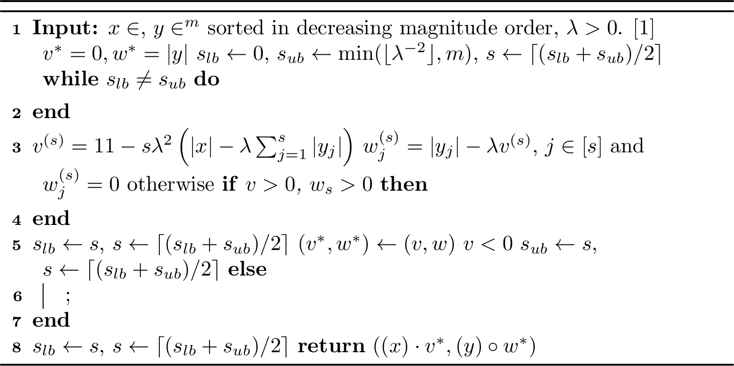
Theorem 3 (Prox computation). Let \((v^*_i, W^*_{i,:})\) be the output of Algorithm 2 with input \(x_i, Y_{i,:}, \lambda\), assuming that each \(Y_{i,:}\) is sorted in decreasing magnitude order. Then \((v^*,W^*)\) is a solution to 4 .
Proof. For any \(i=1,2,\ldots,n\), let \((v^*_i, W^*_{i,:})\) be the output of Algorithm 2 with input \(x_i, Y_{i,:}, \lambda\). We will show that \((v^*,W^*)\) is an optimal solution to 4 by arguing that Algorithm 2 chooses the point with the smallest \(h_\lambda\) value out of a feasible set of solutions containing an optimal solution of 4 .
For simplicity, and without loss of generality, let us consider the one-coordinate-one-row case, that is, \((v^*_i, W^*_{i,:}) \equiv (v^*, w^*)\), \((x_i, Y_{i,:}) \equiv (x, y)\); the proof for the general case is a trivial replication.
By Lemma 2 it is sufficient to prove that \((|v^*|, |w^*|)\) is an optimal solution of 6 , as this will imply the optimality of \((v^*, w^*)\); Recall that Lemma 1 establishes that there exists an optimal solution to 6 .
If the trivial solution is the only optimal solution to 6 , then obviously it will be the output of Algorithm 2. Otherwise, the point described in Corollary 2 is an optimal solution. Assume that Algorithm 2 returned the point \((v^{(s_{\text{out}})},w^{(s_{\text{out}})})\) for some \(s_{\text{out}}\in [\bar{s}]\), meaning in particular that \((v^{(s_{\text{out}})},w^{(s_{\text{out}})})>0\). By definition, \(s^*\geq s_{\text{out}}\). If \(s_{\text{out}}< s^*\), then at some \(s<s^*\) we had that \(v^{(s)}<0\). Since the value of \(v^{(i)}\) is monotonic decreasing in the sparsity level, this implies that \(v^{(s^*)}<0\), which is a contradiction.
Hence, if Algorithm 2 did not return the trivial solution, then \((v^*,w^*) = (v^{(s^*)},w^{(s^*)})\), meaning that \((sign(x) \cdot v^*, sign(y) \circ w^*)\) is a solution to 4 . ◻
4.0.0.1 Time complexity of Algorithm 2
In the worst case where \(m \leq \lambda^{-2}\), the number of searches for finding \(s^*\) is at most \(\log_2(m)\). Each search requires to compute \(v^{(s)}\), and in particular \(\sum_{j=1}^s |y_j|\), as well as \(w_j^{(s)}\), \(j=1,\ldots,s\), each taking \(\mathcal{O}(s)\) steps. Thus, the overall loop complexity is \(\mathcal{O}(m)\).
Moreover, this algorithm assumes that the input vector \(y\) is already sorted in decreasing magnitude order. This can easily be achieved by a sorting procedure in time \(\mathcal{O}(m \log m)\).
5 Multi-Output↩︎
The efficient computation of the robust-sparse proximal mapping we derived for the single-output scenario will now be generalized to the multi-output case. Although we use similar arguments and insights, the analysis is much more complicated and requires more delicate and advanced treatment. Due to the tedious computations that accompany the analysis, the proofs are deferred to appendix 12.
When the network has multiple-output, the proximal operator \(\text{prox}_{\lambda g}(X,Y)\) can be written as the solution set of \[\label{eq:multi-prox} \begin{align} \min_{V,W} \|V - X\|_F + \|W - Y\|_F + 2\lambda \sum_{i=1}^n\sum_{j=1}^m\sum_{k=1}^p |W_{ij}V_{ik}|, \end{align}\tag{7}\] where \(V\in \mathbb{R}^{n\times p}\) and \(W\in \mathbb{R}^{n\times m}\). As in the single-output case, we observe that the proximal mapping 7 is separable with respect to the \(i\)-th rows of the matrices \(V\) and \(W\), and that the signs of the decision variables are determined by the signs of \((X,Y)\). Therefore, it is enough to consider the problem related to the \(i\)-th row of \(V\), denoted as \(x\), and \(i\)-th row of \(W\), denoted as \(y\), i.e., \[\label{eq:5} \begin{align} \min_{v, w \in \mathbb{R}_+^p \times \mathbb{R}_+^m} h_\lambda(v,w;x,y), \end{align}\tag{8}\] where we redefine \(h_\lambda(v,w;x,y)\) to include the multi-output case: \(h_\lambda(v,w;x,y) = \frac{1}{2} \sum_{k=1}^p (v_k-|x_k|)^2 + \frac{1}{2} \sum_{j=1}^m (w_j - |y_j|)^2 + \lambda \sum_{k=1}^p v_k \sum_{j=1}^m w_j.\) To improve readability, we will abuse notation and just write \(h_\lambda(v,w)\), assuming that \((x,y)\) are understood from context.
Using the same observations we exploited to enumerated all stationary points of the proximal mapping in the single-output setup, we can identify the stationary points depending on the number of non zero elements of \(v\) and \(w\).
Lemma 7. Let \((v^*, w^*)\in \mathbb{R}_+^p\times\mathbb{R}_+^m\) be an optimal solution of 12 for a given \((x,y)\in \mathbb{R}\times\mathbb{R}^m\). Then
The vector \(w^*\) satisfies that for any \(j,l\in [m]\) it holds that \(w^*_j \geq w^*_l\) only if \(|y_j| \geq |y_l|\).
The vector \(v^*\) satisfies that for any \(k,l\in [p]\) it holds that \(v^*_k \geq v^*_l\) only if \(|x_k| \geq |x_l|\).
Let \(\bar{x}, \bar{y}\) be the sorted vectors in descending magnitude order of \(x\) and \(y\) respectively. Let \(s_v = |\{k : v_k^* > 0\}|\) and \(s_w = |\{j : w_j^* > 0\}|\). If \(v^*, w^* \neq 0\), then we have that for any \(k \in \{k : v_k^* > 0\}\) and \(j \in \{j : w_j^* > 0\}\), it holds that \(v^* = v^{(s_v, s_w)}\) and \(w^* = w^{(s_v, s_w)}\) where
\[\begin{align} \label{eq:vopt-multi} v_k^{(s_v, s_w)} &= |x_k| + \mu \left(\lambda^2 s_w \sum_{l=1}^{s_v} |\bar{x}_l| - \lambda\sum_{j=1}^{s_w} |\bar{y}_j|\right) \\ \label{eq:wopt-multi} w_j^{(s_v, s_w)} &= |y_j| + \mu \left(\lambda^2 s_v \sum_{l=1}^{s_w} |\bar{y}_l| - \lambda\sum_{k=1}^{s_v} |\bar{x}_k|\right) \end{align}\] {#eq: sublabel=eq:eq:vopt-multi,eq:eq:wopt-multi} and \(\mu = (1 - s_v s_w \lambda^2)^{-1}\).
From the two first points in Lemma 7, the argument in Remark 5 is also valid in the multi-output case, and so we assume hereafter that the input vectors \(x, y\) are sorted in decreasing magnitude order.
Using the second order stationary conditions, we can generalize our sparsity bound in the single-output scenario, given in Lemma 4, to an upper bound on the product of the sparsities of the solutions based on the value of \(\lambda\); indeed, \(s_v = 1\) yields the bound in Lemma 4.
Lemma 8 (Sparsity bound). Let \((v^*, w^*)\in \mathbb{R}_+^p\times\mathbb{R}_+^m\) be an optimal solution of 8 for a given \((x,y)\in \mathbb{R}^p\times\mathbb{R}^m\). Denote \(s_v = | \{ j : w^*_j > 0 \}|\) and \(s_w = |\{j : w_j^* > 0\}|\). Then \(s_v s_w \leq \lambda^{-2}\).
A possible algorithm for computing this proximal mapping would thus be to compute the value of \(h_\lambda \left(v^{(s_v, s_w)},w^{(s_v, s_w)}\right)\) for each pair of sparsities \((s_v, s_w) \in \{0,\ldots,p\} \times \{0,\ldots,m\}\) satisfying \(s_v s_w \leq \lambda^{-2}\) and return the pair achieving the smallest value.
However, such an approach would be computationally inefficient. In order to avoid computing the value of \(h_\lambda\) at each pair, we show the following monotonicity property of \(h_\lambda\) in the sparsity levels, which generalizes the same property in the single-output case.
Lemma 9. Given \((x,y)\in \mathbb{R}^p\times\mathbb{R}^m\), for all \(s_v, s_w \in \{0,\ldots,p\} \times \{0,\ldots,m\}\) satisfying \(s_v s_w < \lambda^{-2}\), we have \[\begin{align} h_\lambda(v^{(s_v, s_w)}, w^{(s_v, s_w)}) &< h_\lambda(v^{(s_v, s_w-1)}, w^{(s_v, s_w-1)}), \\ h_\lambda(v^{(s_v, s_w)}, w^{(s_v, s_w)}) &< h_\lambda(v^{(s_v-1, s_w)}, w^{(s_v-1, s_w)}). \end{align}\]
Moreover, the feasibility criterion \(v \geq 0, w \geq 0\) also has a monotonic property:
Lemma 10. Let \((k,l) \in [p] \times [m]\) be such that \(kl \leq \lambda^{-2}\).
If \(v^{(k, l)} \geq 0\) and \(w^{(k, l)} \geq 0\), then, \(v^{(i, j)} \geq 0\) and \(w^{(i, j)} \geq 0\) \(\forall i = 1, \ldots, k\) and \(\forall j = 1, \ldots, l\).
To properly address the complications arising from handling two intertwining sparsity levels at the same time, we introduce the notion of maximal feasibility boundary (MFB) which acts a frontier of possible sparsity levels.
Definition 1 (Maximal feasibility boundary). We say that a sparsity pair \((s_v,s_w) \in \{0,\ldots,p\} \times \{0,\ldots,m\}\) is on the maximal feasibility boundary (MFB) if incrementing either \(s_v\) or \(s_w\) results with a non-stationary point. That is, if both of the following conditions hold:
\(\bullet\) \(v^{(s_v + 1, s_w)}_{s_v + 1} < 0\) or \(w^{(s_v + 1, s_w)}_{s_w} < 0\) or \((s_v+1)s_w > \lambda^{-2}\),
\(\bullet\) \(v^{(s_v, s_w+1)}_{s_v} < 0\) or \(w^{(s_v, s_w+1)}_{s_w+1} < 0\) or \(s_v(s_w+1) > \lambda^{-2}\).
The efficient computation of the multi-output robust-sparse proximal mapping is based on the fact that we only need to compute the value of \(h_\lambda\) for sparsity levels that are at the frontier of the MFB. This allows us to find the optimal sparsity in time \(\mathcal{O}(p + m)\), improving upon the \(\mathcal{O}(pm)\) complexity of the exhaustive search. Algorithm 3 implements the above by employing a binary search type procedure defined in Algorithm 5 to calculate the MFB.
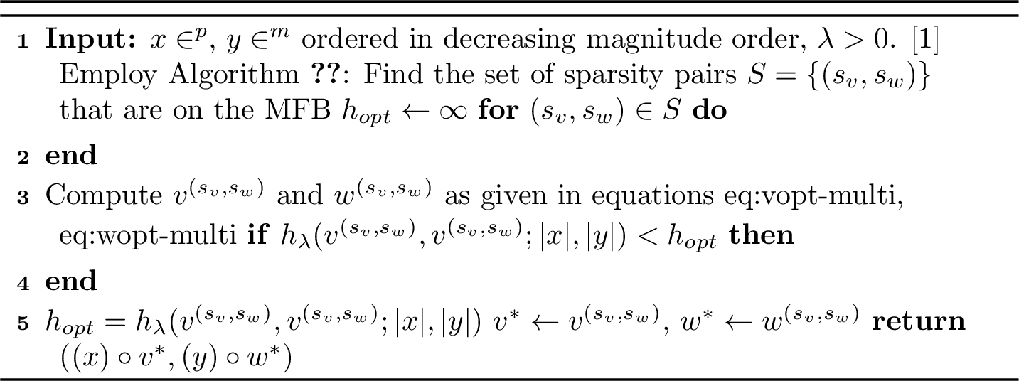
Theorem 4 (Multi-output prox computation). Let \((V^*_{:,i}, W^*_{i,:})\) be the output of Algorithm 3 with input \(X_{:,i}, Y_{i,:}, \lambda\), where each \(X_{:,i}\), \(Y_{i,:}\) are sorted in decreasing magnitude order. Then \((V^*,W^*)\) is a solution to 4 .
5.0.0.1 Time complexity of Algorithm 3
It is easy to see that the maximal feasibility boundary contains at most \(\min(m,p)\) pairs, and Algorithm 5 finds them all in time \(\mathcal{O}(m+p)\). Then, for each such pair \((s_v, s_w)\), we must compute \(v^{(s_v, s_w)}\) and \(w^{(s_v, s_w)}\) and \(h_\lambda(v^{(s_v, s_w)}, w^{(s_v, s_w)})\), which takes time \(\mathcal{O}(m+p)\). The total complexity of Algorithm 3 is thus \(\mathcal{O}(\min(m,p)(m+p))\). In most practical application, the output layer size \(p\) can be considered \(\mathcal{O}(1)\), so that the complexity of computing this proximal mapping is comparable to the complexity of computing one stochastic gradient.
6 Related Work↩︎
The path regularization approach to train neural networks can be traced back to the seminal paper by [11], who introduced the \(p\)-path-norm as a heuristic proxy to control the capacity of the network.
In this paper (cf. 1), we took a step forward by moving from heuristic explanations to rigorous arguments by establishing a new connection between the \(1\)-path-norm and the Lipschitz constant of the network. This result also reads as a relation between the 1-path-norm and the product bound, of which variants have been found to be useful in deriving generalization bounds [6].
Generalization bounds in terms of the \(p\)-path-norm were also derived in [11], but the question of how to methodologically exploit these as regularizers remains open; our algorithmic contribution is a first step in this direction. Additionally, issues regarding optimization with path-norm regularization were reported by [27], which examined a conditional gradient method in the context of path-norm regularization.
A growing collection of works have focused on the task of network compression, doing so via sparsity-inducing regularizers [28]–[31]. They have achieved a great level of success by setting the regularization term in an ad-hoc manner. In contrast, we follow a principled regularization approach with theoretical properties of generalization and robustness, and as a consequence, we are able to quantify the sparsity of the resulting networks.
Moreover, the aforementioned works only use convex regularizers for which efficient proximal mappings are available (see [20] and references therein). We tackle the much harder non-convex regularization task, and derive a new method to compute the proximal mapping in this case. The merits of non-convex non-smooth regularization, and difficulties regarding their optimization, have been extensively studied in the imaging and signal sciences, see e.g., [32] and the recent survey [33].
Layer-wise constraints or regularization with matrix-norms, which are also motivated by the product bound, have been used for robust training [5], [34] and generative models [7]. These focus on robustness with respect to the \(\ell_2\)-norm, which requires a careful handling of operations on the singular values of the weight matrices, and does not have the extra benefit of inducing sparsity.
In 7 we compare to this class of methods for the \(\ell_\infty\)-norm case, in which a simple rescaling of the rows in the weight matrices yields a numerically stable procedure [35], [36].
7 Experiments↩︎
We empirically evaluate shallow neural networks trained by regularized empirical risk minimization 3 using cross-entropy loss. In terms of the weight matrices \(V\) and \(W\) of the network 1 , the following regularizers are considered:
\(\ell_1\) regularization. We penalize the \(\ell_1\)-norm of the parameters of the network, i.e., \(g(V, W) = \| \mathop{\mathrm{vec}}(V)\|_1 + \| \mathop{\mathrm{vec}}(W) \|_1\) in the objective function 3 .
1-path-norm regularization. We set \(g(V, W)\) as \(\sum_{i=1}^n\sum_{j=1}^m\sum_{k=1}^p |W_{ij}V_{ki}|\) in the objective function 3 .
Layer-wise regularization (Parseval Networks). we minimize the cross-entropy loss with a hard constrain on the \(\ell_\infty\)-operator-norm of the weight matrices i.e., \(\|W\|_\infty \leq \lambda^{-1}\) and \(\|V\|_\infty \leq \lambda^{-1}\), as described by [5]. The projection on such set is achieved by projecting each row of the matrices onto an \(\ell_1\)-ball using efficient algorithms [35], [36].
Remark. We will refer (incorrectly) to the training loop defined by PyTorch’s SGD optimizer as Stochastic gradient descent (SGD) (see the discussion in 1).
Experimental setup. Our benchmarks are the MNIST [37], Fashion-MNIST [38] and Kuzushiji-MNIST [39]. For a wide range of learning rates, number of hidden neurons and regularization parameters \(\lambda\), we train networks with SGD and Proximal-SGD (with constant learning rate). We do so for 20 epochs and with batch size set to 100. For each combination of parameters we train 6 networks with the default random initialization. Details and further experiments are reported in appendix 13.
7.1 Convergence of SGD vs Proximal-SGD↩︎
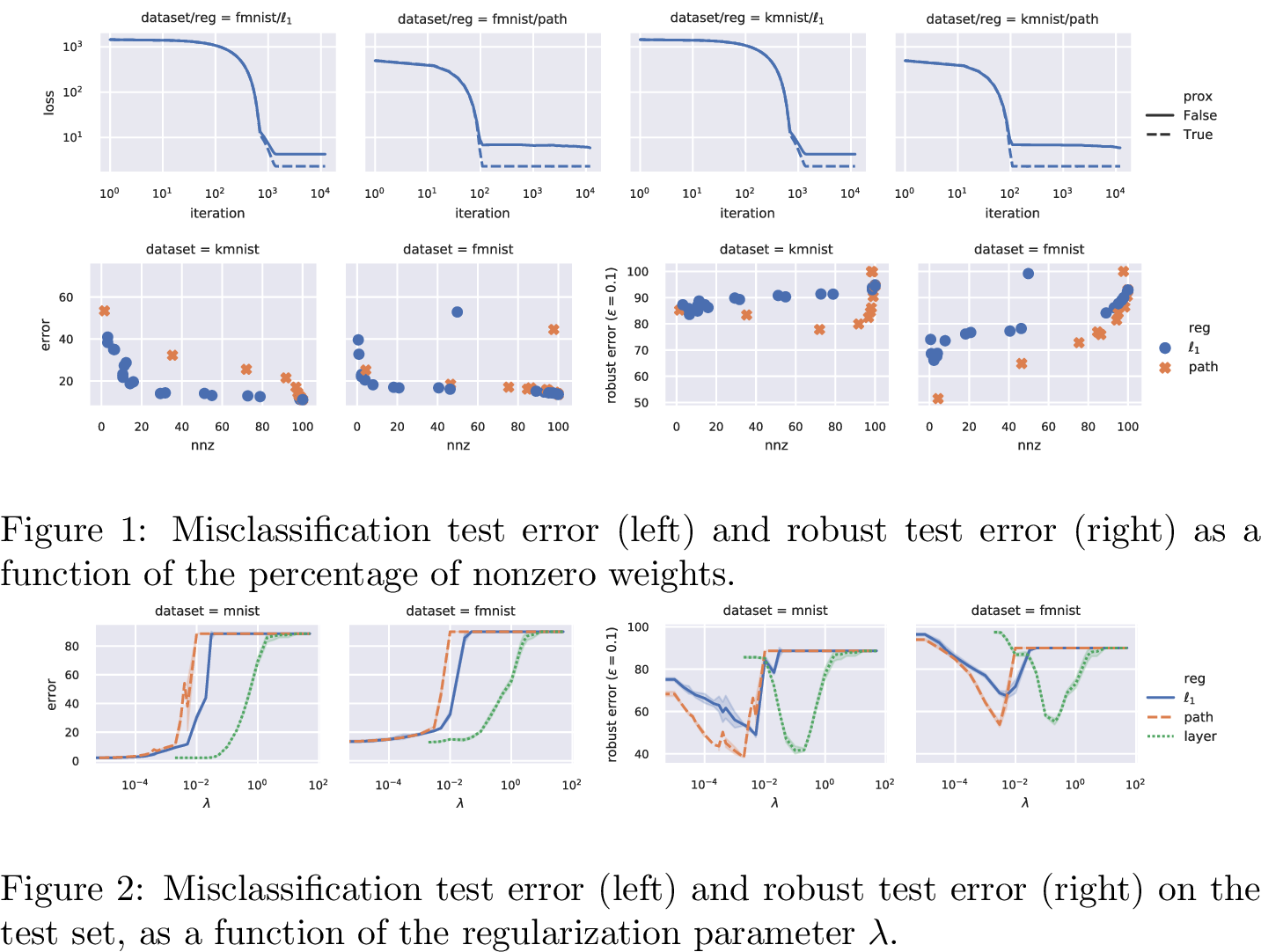
Due to the non-differentiability of the \(\ell_1\)- and path-norm regularizers, we expect Proximal-SGD to converge faster, and to lower values of the regularized loss, when compared to SGD. This is examined in Figure 4, where we plot the value of the loss function across iterations. For both SGD and Proximal-SGD, the loss function decays rapidly in the first few epochs. We then enter a second regime where SGD suffers from slow convergence, whereas Proximal-SGD continues to reduce the loss at a fast rate. At the end of the 20-epochs, Proximal-SGD consistently achieves a lower value of the loss.
An advantage of Proximal-SGD over plain SGD is that the proximal mappings of both the \(\ell_1\)- and path-norm regularizers can set many weights to exactly zero. In [fig:nnz95vs95iter] we plot the average error and robust test error obtained, as a fuction of the sparsity of the network. Compared to \(\ell_1\) regularization, the sparsity pattern induced by the 1-path-norm correlates with the robustness to a higher degree. As a drawback, it appears that in more difficult datasets like KMNIST, the 1-path-norm struggles to obtain good accuracy and sparsity simultaneously.
7.2 The robustness-accuracy trade-off↩︎
The relation between the Lipschitz constant of a network and its robustness to adversarial perturbations has been extensively studied in the literature. In 1 we have shown that the 1-path-norm of a single-output network is a tighter upper bound of its Lipschitz constant, compared to the corresponding product bound.
To the best of our knowledge, the \(\ell_1\)-norm regularizer only provides an upper boud on the already loose product bound [11], which makes it less attractive as a regularizer, despite its sparsity-inducing properties. Hence, the 1-path-norm regularizer is, in theory, a better proxy for robustness than the other regularization schemes.
[fig:error95vs95robust] shows the misclassification error on clean and adversarial examples as a function of \(\lambda\), and corresponds to the learning rate minimizing the error on clean samples. The adversarial perturbations were obtained by PGD [3].
Any training procedure which promotes robustness of a classifier may decrease its accuracy, and this effect is consistently observed in practice [40]. Hence, the merits of a regularizer should be measured by how efficiently it can trade-off accuracy for robustness. We observe that for all three regularization schemes, there exists choices of \(\lambda\) that attain the best possible error on clean samples.
On the other hand, the error obtained by the \(\ell_1\) regularization degrades significantly. The layer-wise and 1-path-norm regularization achieve a noticeably low error on adversarial examples. Comparing the latter schemes, the 1-path-norm regularization shows only a slight advantage over the layer-wise methods, which merits further investigation.
8 Future Work: Multilayer Extension↩︎
A natural extension of our approach is to apply path regularization to multi-layered networks. Since the number of paths is potentially huge, this scenario requires more sophisticated treatment, and hence left for future research. Nonetheless, a trivial extension of our approach is to divide a multi-layered network into pairs of consecutive layers, and apply our method in a sensible manner. We now describe this approach, to complement the theory.
Precisely, assume that the network contains an even number of layers. For some lists of matrices \(\mathbf{V}=(V^1,\ldots, V^k)\) and \(\mathbf{W}=(W^1, \ldots, W^k)\) of appropriate sizes, the network can be written as a composition of activation functions and shallow networks \[h_{\mathbf{V}, \mathbf{W}}:=h_{W^l, V^l} \circ \sigma \circ h_{W^{l-1}, V^{l-1}} \circ \ldots \circ \sigma \circ h_{V^1, W^1}\]
We build the regularized objective as \[\label{eq:objective95multilayer} \min_{\mathbf{V}, \mathbf{W}} \mathbb{E}_{(x, y)}[\ell(h_{\mathbf{V}, \mathbf{W}}(x), y)] + \lambda \sum_{l=1}^L P_1(V^l, W^l).\tag{9}\] where we have introduced the shorthand \[P_1(V^l, W^l):= \sum_{i=1}^{n_l} \sum_{j=1}^{m_l} \sum_{k=1}^{p_l} |W^l_{ij} V^l_{ik}|\] For the 1-path-norm of the \(l\)-th subnetwork \(h_{W^{l}, V^l}\).
Because the nonsmooth nonconvex regularizer in 9 is separable in the variables \(\{(V_i, W_i): i=1,\ldots,k\}\), its proximal mapping is indeed nothing but our multioutput prox algorithm (section 5), applied independently to each shallow subnetwork component. Thus, the proximal gradient methods can be applied efficiently to optimize 9 .
Acknowledgements↩︎
This work is funded (in part) through a PhD fellowship of the Swiss Data Science Center, a joint venture between EPFL and ETH Zurich. This project has received funding from the European Research Council (ERC) under the European Union’s Horizon 2020 research and innovation programme (grant agreement n. 725594 - time-data). This work was supported by the Swiss National Science Foundation (SNSF) under grant number 200021_178865 / 1.
9 Proof of Theorem 1↩︎
We will first prove a particular case of 1, the single-output case (\(p=1\)).
Proposition 1. Let \(h_{V,W}(x)=V^T \sigma(Wx): \mathbb{R}^m \to \mathbb{R}\) be a neural network where \(V \in \mathbb{R}^{n \times 1}\) and \(W \in \mathbb{R}^{n \times m}\). Suppose that that the derivative of the activation is globally bounded between zero and one. Its Lipschitz constant with respect to the \(\ell_\infty\) norm (for the input space) and the \(\ell_1\)-norm (for the output space) is bounded as follows: \[\label{eq:upper95bound95app} L_{V,W} \leq \sum_{i=1}^n \sum_{j=1}^m |W_{i,j} V_{i,1}| \leq \|V\|_1 \|W\|_\infty\qquad{(5)}\]
First, note that because the output space is \(\mathbb{R}\), the \(\ell_1\)-norm is just the absolute value of the output. In this case the Lipschitz constant of the single-output function \(h\) is equal to the supremum of the \(\ell_1\)-norm of its gradient, over its domain (c.f., [9]).
Proof. \[\begin{align} L_{V,W} &= \displaystyle\mathop{\rm sup}_x \| \nabla h_{V,W}(x) \|_1 \\ &= \displaystyle\mathop{\rm sup}_x \displaystyle\mathop{\rm sup}_{\|t \|_\infty \leq 1} t^T \nabla h_{V,W}(x) \\ &= \displaystyle\mathop{\rm sup}_x \displaystyle\mathop{\rm sup}_{\|t \|_\infty \leq 1} t^T W^T \sigma'(Wx)V \\ &\leq \displaystyle\mathop{\rm sup}_{0 \leq s \leq 1} \displaystyle\mathop{\rm sup}_{\|t\|_\infty \leq 1} t^T W^T \mathop{\mathrm{Diag}}(s) V \\ &= \displaystyle\mathop{\rm sup}_{0 \leq s \leq 1} \displaystyle\mathop{\rm sup}_{\|t\|_\infty \leq 1} \sum_{i=1}^n \sum_{j=1}^m t_i (W^T \mathop{\mathrm{Diag}}(V))_{i,j} s_j \\ &\leq \sum_{i=1}^n \sum_{j=1}^m \displaystyle\mathop{\rm sup}_{0 \leq s_j \leq 1} \displaystyle\mathop{\rm sup}_{-1 \leq t_i \leq 1} t_i (W^T \mathop{\mathrm{Diag}}(V))_{i,j}s_j \\ &= \sum_{i=1}^n \sum_{j=1}^m | W^T \mathop{\mathrm{Diag}}(V) |_{i,j} = \sum_{i=1}^n \sum_{j=1}^m |W_{i, j} V_{i, 1}| \end{align}\] This shows the first inequality in ?? . We now show the second inequality. Denote the \(i\)-th row of the matrix \(W\) as \(w_i\): \[\begin{align} \sum_{i=1}^n \sum_{j=1}^m |W_{i, j} V_{i, 1}| &= \sum_{i=1}^n |V_{i, 1}| \sum_{j=1}^m |W_{i,j}| \\ &= \sum_{i=1}^n |V_{i, 1}| \|w_i\|_1 \\ &\leq \sum_{i=1}^n |V_{i, 1}| \max_{j=1, \ldots, m} \|w_j\|_1 \\ &=\sum_{i=1}^n |V_{i, 1}| \|W\|_\infty \\ &= \|V\|_1 \|W\|_\infty \end{align}\] In the fourth line we have used the fact that the \(\ell_\infty\) operator norm of a matrix is equal to the maximum \(\ell_1\)-norm of the rows. ◻
Proof of 1. We now proceed with the general case where \(V \in \mathbb{R}^{n \times p}\), \(W \in \mathbb{R}^{n \times m}\) and \(h_{V,W}(x)=V^T \sigma(Wx)\).
Proof. Denote the columns of \(V\), in order, as \(V_1, \ldots, V_p\). Using 1 we have \[\begin{align} \| V^T \sigma(Wx) - V^T \sigma(Wy)\|_1 &= \sum_{k=1}^p |V_k^T \sigma(Wx) - V_k^T \sigma(Wy)| \\ & \leq \sum_{k=1}^p \sum_{i=1}^n \sum_{j=1}^m |W_{i, j} V_{i, k} | \|x - u \|_\infty \\ & \leq \sum_{k=1}^p \|V_k\|_1 \|W \|_\infty \|x - y \|_\infty \\ &= \|V^T\|_{\infty, 1} \|W \|_\infty \|x - y \|_\infty \end{align}\] where in the fourth line we have used the fact that the \((\ell_\infty, \ell_1)\) operator norm of a matrix \(V^T\) is equal to the sum of the \(\ell_1\) norm of its rows i.e., the columns of \(V\). This shows that \(L_{V,W} \leq \sum_{i=1}^n \sum_{j=1}^m \sum_{k=1}^p |W_{i, j} V_{i, k}| \leq \|V^T\|_{\infty, 1} \|W \|_\infty\) ◻
10 Proof of Theorem 2↩︎
In this section we prove the theoretical guarantees stated in Theorem 2 of the prox-grad method described by Algorithm 1. The first and second parts of Theorem 2 follow immediately from the results establish by [12]. Part two in Theorem 2 states that Algorithm 1 is globally convergent under the celebrated Kurdyka–Lojasiewicz (KL) property [41]. The broad classes of semi-algebraic and subanalytic functions, widely used in optimization, satisfy the KL property (see e.g. [12]), and in particular, most convex functions encountered in finite dimensional applications satisfy it (see [12]). We refer the reader to the works [12], [41], [42], in particular to [12] for additional information and results.
For Part three we require the sufficient decrease property stated next.
Lemma 11 (Sufficient decrease property [12]). Let \(\Psi : \mathbb{R}^n\rightarrow\mathbb{R}\) be a continuously differentiable function with gradient assumed \(L_\Psi\)-Lipschitz continuous, and let \(\sigma :\mathbb{R}^n\rightarrow (-\infty,\infty]\) be a proper l.s.c function satisfying that \(\displaystyle\mathop{\rm inf}\sigma>-\infty\). Fix any \(t \in (0, 1/L_\Psi)\). Then, for any \({\boldsymbol{u}}\in\displaystyle\mathop{\rm dom}\sigma\) and any \({\boldsymbol{u}}^+\in\mathbb{R}^n\) defined by \[{\boldsymbol{u}}^+\in\mathrm{prox}_{\sigma t} \left({\boldsymbol{u}}- t \nabla\Psi ({\boldsymbol{u}}) \right)\] we have \[\Psi ({\boldsymbol{u}}) + \sigma({\boldsymbol{u}})- \Psi ({\boldsymbol{u}}^+) -\sigma({\boldsymbol{u}}) \geq \frac{ 1 - t L_\Psi}{2 t} \|{\boldsymbol{u}}^+ - {\boldsymbol{u}}\|^2.\]
Proof of Theorem 2. The first and second parts follow from the results established by [12]. We will now prove the third part. By Lemma 11 we have that \[\label{eq:4} \mathcal{F}(z^k) - \mathcal{F} (z^{k+1}) = f (z^k) + \lambda g(z^k) - f (z^{k+1}) - \lambda g(z^{k+1})) \geq \frac{1 - L \eta_k}{2 \eta_k} \|z^{k+1} - z^k \|^2.\tag{10}\] Hence \(\{ f (z^k) + \lambda g(z^k) \}_{k\geq 0}\) is a non-increasing sequence that strictly decreasing unless a critical point is obtained in a finite number of steps. By summing 10 over \(k=0,1,\ldots,K\) and using the fact that \(\{ f (z^k) + \lambda g(z^k) \}_{k\geq 0}\) is non-increasing and is bounded below by \(\mathcal{F}_*\), we obtain that \[\begin{align} \mathcal{F}(z^0) - \mathcal{F}_* &\geq \sum_{k=0}^{K}\frac{1 - L \eta_k}{2 \eta_k} \|z^{k+1} - z^k \|^2 \\ &\geq \frac{1}{2}(c - L) K \min_{k=0,\dots,K} \|z^{k+1} - z^k \|_2^2. \end{align}\] Consequently, \[\min_{k=0,\dots,K} \|z^{k+1} - z^k \|_2 \leq \sqrt{\frac{2(\mathcal{F}(z^0) - \mathcal{F}_*)}{(c-L)K}}.\] ◻
11 Single output proximal map computation↩︎
This section provides the theoretical background and the required intermediate results to prove Theorem 3.
11.1 Moving to an Equivalent Easier Problem↩︎
We are interested in minimizing the nonconvex twice continuously differentiable function \[\label{eq:7} \min_{v, w\in\mathbb{R}\times\mathbb{R}^m} \frac{1}{2} (v-x)^2 + \frac{1}{2} \sum_{j=1}^m (w_j - y_j)^2 + \lambda |v| \sum_{j=1}^m |w_j|.\tag{11}\] The signs of the elements of the decision variables in (11 ) are determined by the signs of \((x, y)\), and consequently, the problem in (11 ) is equivalent to problem 12 ; this is (partly) formulated by Lemma 12. \[\label{eq:8} \min_{v, w\in\mathbb{R}_+\times\mathbb{R}_+^m} h_\lambda(v,w;x,y) \equiv \frac{1}{2} (v-|x|)^2 + \frac{1}{2} \sum_{j=1}^m (w_j - |y_j|)^2 + \lambda v \sum_{j=1}^m w_j.\tag{12}\]
Lemma 12. Let \((v^*, w^*)\in\mathbb{R}_+\times\mathbb{R}_+^n\) be an optimal solution of problem 12 . Then \((sign(x) \cdot v^*, sign(y) \circ w^*)\) is an optimal solution of problem 11 .
Proof. We have that \[\begin{align} \tilde{h}_\lambda(v,w;x,y) &\equiv \frac{1}{2} (v-x)^2 + \frac{1}{2} \sum_{j=1}^m (w_j - y_j)^2 + \lambda |v| \sum_{j=1}^m |w_j|\\ &= \frac{1}{2} ( sign(x) v-|x|)^2 + \frac{1}{2} \sum_{j=1}^m (sign(y_j) w_j - |y_j|)^2 + \lambda |v| \sum_{j=1}^m |w_j|\\ &\geq \frac{1}{2} (|v|-|x|)^2 + \frac{1}{2} \sum_{j=1}^m (|w_j| - |y_j|)^2 + \lambda v \sum_{j=1}^m w_j \\ &\geq h_\lambda(v^*,w^*;|x|,|y|), \end{align}\] where the last inequality follows from the fact that \((v^*, w^*)\) is an optimal solution of 12 . Since equality with the lower bound is attained by setting \((v,w) = (sign(x) \cdot v^*, sign(y) \circ w^*)\), we conclude that \((sign(x) \cdot v^*, sign(y) \circ w^*)\) is an optimal solution of 11 . ◻
To summarize, we have established that, finding an optimal solution to 12 and then changing signs accordingly, yields an optimal solution to 11 . We will now focus on obtaining an optimal solution for (11 ).
11.2 Solving the Prox Problem↩︎
First we note that problem 12 is well-posed.
Lemma 13 (Well-posedness of 12 ). For any \(\lambda\geq 0\) and any \((x,y)\in\mathbb{R}\times\mathbb{R}^m\), the problem 12 has a global optimal solution.
Proof. The claim follows from the fact that the objective function is coercive, cf. [24]. ◻
In light of Lemma 13, and due to the fact that in 12 we minimize a continuously differentiable function over a closed convex set, the set of optimal solutions of 12 is a nonempty subset of the set of stationary points of 12 . These satisfy the following conditions (cf. [24]).
Lemma 14 (Stationarity conditions). Let \((v^*, w^*)\in \mathbb{R}_+\times\mathbb{R}_+^m\) be an optimal solution of 12 for a given \((x,y)\in \mathbb{R}\times\mathbb{R}^m\). Then \[\begin{align} w_j^* &= \max \left\lbrace 0, |y_j| - \lambda v^* \right\rbrace \;\text{ for any } j=1,2,\ldots,m,\\ v^* &= \max\left\lbrace 0, |x| - \lambda \sum_{j=1}^{m} w^*_j \right\rbrace. \end{align}\]
Proof. The stationarity (first-order) conditions of 12 (cf. [24]) state that \[\begin{align} \frac{\partial h_\lambda}{\partial v}(v^*,w^*;x,y) \begin{cases} = 0, & v^*>0,\\ \geq 0, & v^* = 0, \end{cases} \quad \frac{\partial h_\lambda}{\partial w_j}(v^*,w^*;x,y) \begin{cases} = 0, & w_j^*>0,\\ \geq 0, & w_j^* = 0, \end{cases} \end{align}\] which translates to \[\begin{align} v^* - |x| + \lambda \sum_{j=1}^m w^*_j \begin{cases} = 0, & v^*>0,\\ \geq 0, & v^* = 0, \end{cases} \quad w^*_j - |y_j| + \lambda v^* \begin{cases} = 0, & w_j^*>0,\\ \geq 0, & w_j^* = 0, \end{cases} \end{align}\] and the required follows. ◻
The stationarity conditions given in Lemma 14 imply a solution form that we exploit in Algorithm 2; this is described by Corollary 3, where we use the convention that \(\sum_{j=1}^{0} a_j \equiv 0\) for any \(\{a_j\}\subseteq\mathbb{R}\).
Corollary 3. Let \((v^*, w^*)\in \mathbb{R}_+\times\mathbb{R}_+^m\) be an optimal solution of 12 for a given \((x,y)\in \mathbb{R}\times\mathbb{R}^m\).
The vector \(w^*\) satisfies that for any \(j,l\in\{1,2,\ldots,m \}\) it holds that \(w^*_j \geq w^*_l\) only if \(|y_j| \geq |y_l|\).
If \(v^* = 0\), then \(w^* = y\).
If \(v^* > 0\), and \(s = | \{ j : w^*_j > 0 \} |\), then we have that \[\label{eq:2} v^* = \dfrac{1}{1-s \lambda^2}\left(|x| - \lambda\sum_{j=1}^s|\bar{y}_j|\right),\qquad{(6)}\] where \(\bar{y}\) is the sorted vector of \(y\) in descending magnitude order.
Proof. The first part follows trivially from the stationarity conditions on \(w^*\) given in Lemma 14. The second part also follows trivially from the problem definition.
From the first part and the conditions in Lemma 14 we have that \(\sum_{j=1}^{m} w^*_j = \sum_{j=1}^s|\bar{y}_j| - \lambda s v^*\). Plugging the latter to the stationarity condition on \(v^*\) (given in Lemma 14) then implies the required. ◻
In our analysis, we strictly distinguish between the trivial solution \((v^*,w^*) = (0,y)\), and the non-trivial solution in which \(v^*>0\). A practical point-of-view suggests that if \(v^* = 0\), then the corresponding succeeding weights should also be zero, even though the optimality conditions imply otherwise. However, to avoid hindering the training process, this observation is considered only in the end of the training.
Recall that our analysis so-far implies that the magnitude order of \(y\) determines the order magnitude of \(w\), effectively implying on set of non-zero entries in \(w\) (cf. Remark 5). For clarity of indices, and without loss of generality, we assume throughout this section that the vector \(y\) is already sorted in decreasing order of magnitude, that is \(y \equiv \bar{y}\). We will use, without confusion, both notation to describe the same entity in order to maintain coherence with our procedures and results.
Denote \[\label{eq:vsws} \begin{align} v^{(s)} &= \dfrac{1}{1-s \lambda^2}\left(|x| - \lambda\sum_{j=1}^s|y_j|\right) \\ w^{(s)}_j &= |y_j| - \lambda v^{(s)} \;\text{ for } j=1,2,\ldots,s, \;\text{ and } w^{(s)}_j = 0 \;\text{otherwise}. \end{align}\tag{13}\] Lemma 5 which states the monotonicity property \[h_\lambda(v^{(s)}, w^{(s)}; x, y) < h_\lambda(v^{(s-1)}, w^{(s-1)}; x, y).\] is proved next.
Proof of Lemma 5. Recall that \(h_\lambda(v,w;x,y) := \frac{1}{2} (v-|x|)^2 + \frac{1}{2} \sum_{j=1}^m (w_j - |y_j|)^2 + \lambda v \sum_{j=1}^m w_j.\) By plugging \(w^{(s)}\) defined in 13 to \(h_\lambda\) we obtain that \[\begin{align} h_\lambda(v^{(s)}, w^{(s)}; x, y) &= \frac{1}{2} (v^{(s)} - |x|)^2 + \frac{1}{2} \sum_{i=1}^s (|\bar{y}_i| - (|\bar{y}_i| - \lambda v^{(s)}))^2 + \frac{1}{2}\sum_{i=s+1}^m |\bar{y}_i|^2 + \lambda v^{(s)} \sum_{i=1}^s (|\bar{y}_i| - \lambda v^{(s)}) \\ &= \frac{1}{2} (v^{(s)} - |x|)^2 + \frac{\lambda^2}{2} s (v^{(s)})^2 + \frac{1}{2} \|y\|_2^2 - \frac{1}{2}\sum_{i=1}^s |\bar{y}_i|^2 + \lambda v^{(s)} \sum_{i=1}^s |\bar{y}_i| - \lambda^2 s (v^{(s)})^2 . \end{align}\] Consequently, plugging \(v^{(s)}\), defined in 13 , yields \[\begin{align} h_\lambda(v^{(s)}, w^{(s)}; x, y) &= \frac{1}{2} \left(\frac{\lambda^2 s}{1 - \lambda^2 s} |x| - \frac{\lambda}{1-\lambda^2 s} \sum_{i=1}^s |\bar{y}_i| \right)^2 - \frac{\lambda^2 s}{2(1- \lambda^2 s)^2} \left( |x| - \lambda \sum_{i=1}^s |\bar{y}_i| \right)^2 \\ &+ \frac{\lambda}{1 - \lambda^2 s}\sum_{i=1}^s |\bar{y}_i| \left(|x| - \lambda \sum_{i=1}^s |\bar{y}_i| \right) - \frac{1}{2} \sum_{i=1}^s |\bar{y}_i|^2 + \frac{1}{2} \|y\|_2^2 \\ &= \frac{\lambda^2 s}{2(1-\lambda^2 s)^2} x^2 (\lambda^2 s - 1) + \frac{\lambda^2}{2(1-\lambda^2 s)^2} \left(\sum_{i=1}^s |\bar{y}_i| \right)^2 (1 - \lambda^2 s - 2(1 - \lambda^2 s)) \\ &+ |x| \sum_{i=1}^s |\bar{y}_i| \left(-\frac{\lambda^3 s}{(1-\lambda^2 s)^2} + \frac{\lambda^3 s}{(1-\lambda^2 s)^2} + \frac{\lambda}{1-\lambda^2 s} \right) - \frac{1}{2} \sum_{i=1}^s |\bar{y}_i|^2 + \frac{1}{2} \|y\|_2^2 \\ &= \frac{1}{2(1 - \lambda^2 s)} \left( -\lambda^2 s x^2 - \left(|x| - \lambda \sum_{i=1}^s |\bar{y}_i| \right)^2 + x^2 \right)- \frac{1}{2} \sum_{i=1}^s |\bar{y}_i|^2 + \frac{1}{2} \|y\|_2^2 \\ &= - \frac{1}{2(1-\lambda^2 s)}\left(|x| - \lambda \sum_{i=1}^s |\bar{y}_i| \right)^2 + \frac{1}{2} \|x\|_2^2 - \frac{1}{2} \sum_{i=1}^s |\bar{y}_i|^2 + \frac{1}{2} \|y\|_2^2 \\ &= - \left(1 + \frac{\lambda^2}{1 - \lambda^2 s}\right)\frac{1}{2(1-\lambda^2 (s-1))}\left(|x| - \lambda \sum_{i=1}^{s-1} |\bar{y}_i| - \lambda |\bar{y}_s| \right)^2 + \frac{1}{2} \|x\|_2^2 - \frac{1}{2} \sum_{i=1}^{s-1} |\bar{y}_i|^2 - \frac{1}{2} |\bar{y}_s|^2 + \frac{1}{2} \|y\|_2^2 \\ &= h_\lambda(v^{(s-1)}, w^{(s-1)}; x, y) - \frac{1}{2(1 - \lambda^2 s + \lambda^2)}\left( -2\lambda |\bar{y}_s| \left( |x| - \lambda \sum_{i=1}^{s-1} |\bar{y}_i| \right) + \lambda^2 |\bar{y}_s|^2\right) \\ &- \frac{\lambda^2}{2(1-\lambda^2 s)(1-\lambda^2 s + \lambda^2)}\left(|x| - \lambda \sum_{i=1}^s |\bar{y}_i| \right)^2 - \frac{1}{2} |\bar{y}_s|^2. \end{align}\] Therefore, \[\begin{align} &h_\lambda(v^{(s)}, w^{(s)}; x, y) - h_\lambda(v^{(s-1)}, w^{(s-1)}; x, y) \nonumber \\ &= - \frac{1}{2(1 - \lambda^2 s + \lambda^2)}\left( -2\lambda |\bar{y}_s| \left( |x| - \lambda \sum_{i=1}^s |\bar{y}_i| \right) - \lambda^2 |\bar{y}_s|^2 + \frac{\lambda^2}{1 - \lambda^2 s}\left( |x| - \lambda \sum_{i=1}^s |\bar{y}_i| \right)^2 + (1- \lambda^2 s + \lambda^2) |\bar{y}_s|^2\right) \nonumber \\ &= - \frac{1}{2(1 - \lambda^2 s + \lambda^2)}\left( (1- \lambda^2 s) |\bar{y}_s|^2 -2\lambda |\bar{y}_s| \left( |x| - \lambda \sum_{i=1}^s |\bar{y}_i| \right) + \frac{\lambda^2}{1 - \lambda^2 s}\left( |x| - \lambda \sum_{i=1}^s |\bar{y}_i| \right)^2\right) \nonumber \\ &= - \frac{1 - \lambda^2 s}{2(1 - \lambda^2 s + \lambda^2)}\left( |\bar{y}_s|^2 -2\lambda |\bar{y}_s| v^{(s)} + \lambda^2(v^{(s)})^2\right) \nonumber \\ &= - \frac{1 - \lambda^2 s}{2(1 - \lambda^2 s + \lambda^2)}\left( |\bar{y}_s| -\lambda v^{(s)} \right)^2 \leq 0, \end{align}\] meaning that \[h_\lambda (v^{(s)}, w^{(s)}; x, y) \leq h_\lambda(v^{(s-1)}, w^{(s-1)}; x, y).\] ◻
We can now prove our key result formulated in Corollary 2, that states that \((v^{(s^*)}, w^{(s^*)} )\) is an optimal solution of 6 for \[s^* = \max \left\lbrace s \in [\bar{s}] : v^{(s)}, w^{(s)} > 0\right\rbrace, \;\text{ where } \;\bar{s} = \min(\lfloor \lambda^{-2}\rfloor, m).\]
Proof of Corollary 2. By Lemma 3, \((v^{(s^*)}, w^{(s^*)} )\) is a stationary point of 6 . Moreover, according to Corollary 1 and Lemma 4, \((v^{(s^*)}, w^{(s^*)} )\) belongs to the set of \(\bar{s}\) stationary points that are candidates to be optimal solutions of 6 . Invoking Lemma 5, we have that \[\label{eq:52} h_\lambda(v^{(s^*)}, w^{(s^*)}; x, y) < h_\lambda(v^{(j)}, w^{(j)}; x, y), \quad \forall s^* > j.\tag{14}\] Hence, \((v^{(j)}, w^{(j)} )\) is not an optimal solution for any \(j<s^*\).
Let us now consider the complementary case. By Lemma 4, for any \(i>\bar{s}\) the pair \((v^{(i)}, w^{(i)} )\) does not satisfy the second-order optimality conditions, and therefore is not an optimal solution. On the other hand, by the definition of \(s^*\), for any \(\bar{s} >i>s^*\) the pair \((v^{(i)}, w^{(i)} )\) is not a feasible solution , and subsequently not a stationary point. To conclude, \(h_\lambda(v^{(s^*)}, w^{(s^*)}; x, y) < h_\lambda(v^{(j)}, w^{(j)}; x, y)\) holds for any \(j\neq s^*\) such that \((v^{(j)}, w^{(j)} )\) is a stationary point, meaning that \((v^{(s^*)}, w^{(s^*)} )\) is an optimal solution of 6 . ◻
Finally, we will show that the problem of finding \(s^*\) can be easily solved using binary search. To this end, we show that the feasibility criterion (i.e., \(v^{(s)} > 0\) and \(w^{(s)} > 0\)) satisfies that \[(v^{(k)}, w^{(k)}) \text{ is feasible } \Rightarrow (v^{(i)}, w^{(i)}) \text{ is feasible } \forall i < k\]
Proof of Lemma 6. Suppose that \((v^{(k)}, w^{(k)})\) is feasible for some \(k \in \{2, \ldots, \bar{s}\}\). By induction principle, it is sufficient to show that \((v^{(k-1)}, w^{(k-1)})\) is feasible in order to prove the result.
By 13 , we have: \[(1-k\lambda^2)v^{(k)} = |x| - \lambda \sum_{j=1}^k |y_j| = (1-k\lambda^2 + \lambda^2)v^{(k-1)} - |y_k|.\] which implies \[v^{(k-1)} = \frac{1}{(1-k\lambda^2 + \lambda^2)}((1-k\lambda^2)v^{(k)} + |y_k|) \geq 0.\]
For \(w^{(k)}\), it is easy to see from 13 that since the vector \(y\) is sorted in decreasing order of magnitude, the vector \(w^{(k)}\) is also sorted in decreasing order, and thus \(w^{(k)}\) is feasible if and only if \(w^{(k)}_k > 0\). \[\begin{align} (1-k \lambda^2)w^{(k)}_k &= (1-k \lambda^2)|y_k| - \lambda |x| + \lambda^2 \sum_{j=1}^k |y_j| \\ &= -\lambda |x| + (1 - (k-1)\lambda^2)|y_{k-1}| + \lambda^2 \sum_{j=1}^{k-1} |y_j| + \lambda^2 |y_k| + (1-k \lambda^2)|y_k| - (1 - (k-1)\lambda^2)|y_{k-1}| \\ &= (1-(k-1) \lambda^2)w^{(k-1)}_{k-1} + (1-k\lambda^2 + \lambda^2)(|y_k| - |y_{k-1}|), \end{align}\] where the last line uses the identity of the first line for \(k-1\). We thus have: \[w^{(k-1)}_{k-1} = \frac{1}{(1-(k-1) \lambda^2)} (1-k \lambda^2)w^{(k)}_k + |y_{k-1}| - |y_k| \geq 0,\] since \(|y_{k-1}| \geq |y_k|\) and \(k \leq \lambda^{-2}\).
Therefore, there exists a value \(s^*\) such that \(v^{(k)} > 0\) and \(w^{(k)} > 0\) \(\forall k \geq s^*\) and \(v^{(k)} \geq 0\) or \(w^{(k)} \geq 0\) \(\forall k > s^*\). This value of \(s^*\) can thus efficiently be found using binary search. ◻
12 Multi-output proximal map computation↩︎
12.1 Solving the prox problem↩︎
Returning to the multi-output setting, recall that \(h_{V,W}(x) = V^T \sigma(Wx)\) with \(V \in \mathbb{R}^{p\times n}, W\in \mathbb{R}^{n\times m}\) and \[g(V, W)= \sum_{i=1}^n\sum_{j=1}^m\sum_{k=1}^p W_{ij}V_{ki}.\] The proximal mapping can then be written as: \[\begin{align} \text{prox}_{\lambda g}(\bar{V}, \bar{W}) &= \displaystyle\mathop{\rm argmin}_{V, W} \frac{1}{2} \|V - \bar{V}\|_F + \frac{1}{2} \|W - \bar{W}\|_F + \lambda \sum_{i=1}^n\sum_{j=1}^m\sum_{k=1}^p W_{ij}V_{ki} \\ &= \displaystyle\mathop{\rm argmin}_{V, W} \sum_{i=1}^n \left( \frac{1}{2} \sum_{k=1}^p (V_{ki} - \bar{V}_{ki})^2 + \sum_{j=1}^p (W_{ij} - \bar{W}_{ij})^2 + \sum_{j=1}^m\sum_{k=1}^p W_{ij}V_{ki}\right). \end{align}\] Noting that the proximal mapping is separable with respect to the columns of \(W\) and the rows of \(V\), and using the same sign trick applied in the single-output case, it is enough to solve for any \(i=1,\ldots, n\), \[\min_{v, w\in \mathbb{R}_+^p \times \mathbb{R}_+^m} h_\lambda(v,w;x,y) \equiv \frac{1}{2} \sum_{k=1}^p (v_k - |x_k|)^2 + \frac{1}{2} \sum_{j=1}^m (w_j - |y_j|)^2 + \lambda \sum_{j=1}^m\sum_{k=1}^p v_k w_j, \label{eq:multi-ouptut-prox}\tag{15}\] where \(x\) denotes the \(i\)-th row of \(V\) and \(y\) the \(i\)-th column of \(W\), in order to compute the prox operator.
The stationarity conditions for 15 are stated next; the arguments are the same as in the single-output case.
Lemma 15 (Stationarity conditions). Let \((v^*, w^*)\in \mathbb{R}_+^p\times\mathbb{R}_+^m\) be an optimal solution of 15 for a given \((x,y)\in \mathbb{R}^p\times\mathbb{R}^m\). Then \[\begin{align} w_j^* &= \max \left\lbrace 0, |y_j| - \lambda \sum_{k=1}^p v_k^* \right\rbrace \;\text{ for any } j=1,2,\ldots,m,\\ v_k^* &= \max\left\lbrace 0, |x_k| - \lambda \sum_{j=1}^{m} w^*_j \right\rbrace \;\text{ for any } k=1,2,\ldots, p. \end{align}\]
The next lemma restates the result in Lemma 7 which expands on the monotonic relation in magnitude originally established for single-output networks in Corollary 1.
Lemma 16. Let \((v^*, w^*)\in \mathbb{R}_+^p\times\mathbb{R}_+^m\) be an optimal solution of 12 for a given \((x,y)\in \mathbb{R}^p \times\mathbb{R}^m\).
The vector \(w^*\) satisfies that for any \(j,l\in\{1,2,\ldots,m \}\) it holds that \(w^*_j \geq w^*_l\) only if \(|y_j| \geq |y_l|\).
The vector \(v^*\) satisfies that for any \(k,l\in\{1,2,\ldots,p \}\) it holds that \(v^*_k \geq v^*_l\) only if \(|x_k| \geq |x_l|\).
Let \(\bar{x}, \bar{y}\) be the sorted vector of \(x\) and \(y\) respectively in descending magnitude order. Let \(s_v = |\{k : v_k^* > 0\}|\) and \(s_w = |\{j : w_j^* > 0\}|\). If \(v^*, w^* \neq 0\), then \[\begin{align} v_k^* &= |x_k| + \dfrac{1}{1 - s_v s_w \lambda^2}\left(\lambda^2 s_w \sum_{l=1}^{s_v} |\bar{x}_l| - \lambda\sum_{j=1}^{s_w} |\bar{y}_j|\right), \\ w_j^* &= |y_j| + \dfrac{1}{1 - s_v s_w \lambda^2}\left(\lambda^2 s_v \sum_{l=1}^{s_w} |\bar{y}_l| - \lambda\sum_{k=1}^{s_v} |\bar{x}_k|\right). \end{align}\]
Proof. The two first points are direct applications of the stationary conditions of Lemma 15.
From the conditions in Lemma 15 we have that \[\begin{align} \sum_{j=1}^{m} w^*_j &= \sum_{j=1}^{s_w} |\bar{y}_j| - \lambda s_w \sum_{k=1}^p v_k^* \\ \sum_{k=1}^{p} v^*_k &= \sum_{k=1}^{s_v} |\bar{x}_k| -\lambda s_v \sum_{j=1}^m w_j^* \\ &= \sum_{k=1}^{s_v} |\bar{x}_k| - \lambda s_v \sum_{j=1}^{s_w} |\bar{y}_j| + \lambda^2 s_v s_w \sum_{k=1}^p v_k^* \\ &= \frac{1}{1-\lambda^2 s_v s_w} \left( \sum_{k=1}^{s_v} |\bar{x}_k| - \lambda s_v \sum_{j=1}^{s_w} |\bar{y}_j| \right). \end{align}\] Thus, \[\begin{align} \sum_{j=1}^{m} w^*_j &= \sum_{j=1}^{s_w} |\bar{y}_j| - \frac{\lambda s_w}{1-\lambda^2 s_v s_w} \left( \sum_{k=1}^{s_v} |\bar{x}_k| - \lambda s_v \sum_{j=1}^{s_w} |\bar{y}_j| \right) \\ &= \frac{1}{1-\lambda^2 s_v s_w} \left( -\lambda s_w \sum_{k=1}^{s_v} |\bar{x}_k| + \sum_{j=1}^{s_w} |\bar{y}_j| \right). \end{align}\]
Plugging the latter to the stationarity condition on \(v^*\) (given in Lemma 15) then implies the result. ◻
Finally, we show, as in the single-output case, that second order stationarity condition constraints the ranges of sparsities of \(v^*\) and \(w^*\); this relation is given by Lemma 8, and is proved next.
Proof of Lemma 8. Since \((v^*, w^*)\) is an optimal solution of 15 and the objective function in 15 is twice continuously differentiable, \((v^*, w^*)\) satisfies the second order necessary optimality conditions. That is, for any \(d\in\mathbb{R}^p\times\mathbb{R}^m\) satisfying that \((v^*, w^*)+d \in \mathbb{R}_+^p\times\mathbb{R}_+^m\) and \(d^T \nabla h_\lambda(v^*, w^*;x,y) = 0\) it holds that \[d^T \nabla^2 h_\lambda(v^*, w^*;x,y)d = d^T \left( \begin{array}{ccc} I_{p\times p} & \Lambda_{p \times m} \\ \Lambda_{m \times p }& I_{m\times m} \end{array} \right) d \geq 0,\] where the first row/column corresponds to \(v\) and the others correspond to \(w\), \(I\) denotes the identity matrix and \(\Lambda\) denotes a matrix completely filled with \(\lambda\). Similarly as in the single output case, we require that the submatrix of \(\nabla^2 h_\lambda(v^*, w^*;x,y)\) containing the rows and columns corresponding to the positive coordinates in \((v^*, w^*)\) is positive semidefinite. Since the minimal eigenvalue of this submatrix equals \(1-\lambda\sqrt{|S_v||S_w|}\), we have that \[\lambda^{-2} \geq |S_v||S_w|.\] ◻
A possible way of solving this proximal problem is thus to exhaustively compute the value of \(h_\lambda\) at each stationary point associated with sparsities \(s_v = 1, \ldots, p\), \(s_w = 1, \ldots, m\) such that \(s_v s_w \leq \lambda^{-2}\). However, trying all possible pairs of sparsities \((s_v, s_w)\) is computationally costly. Similarly as is the single output case, we can exploit some structure of the objective function \(h_\lambda\) in order to reduce the possible candidate pairs of sparsities.
Without loss of generality, we assume hereafter that the vectors \(x, y\) are already sorted in decreasing order of magnitude.
Lemma 16 shows that for each pair \((s_v, s_w)\), \(s_v = 0,1,\ldots,p\), \(s_w = 0,1,\ldots,m\), there exists a stationary point \((v^{(s_v, s_w)}, w^{(s_v, s_w)})\) of \(h_\lambda(\cdot, \cdot; x,y)\) such that \(|\{k: v^{(s_v, s_w)}_k > 0\}| = s_v\), \(|\{j: w^{(s_v, s_w)}_j > 0\}| = s_w\), given by \[\label{eq:vsws-multi} \begin{align} v^{(s_v, s_w)}_k &= |x_k| + \dfrac{1}{1 - s_v s_w \lambda^2}\left(\lambda^2 s_w \sum_{l=1}^{s_v} |x_l| - \lambda\sum_{j=1}^{s_w} |y_j|\right) \;\text{ for } k=1,2,\ldots,s_v, \;\text{ and } v^{(s_v, s_w)}_k = 0 \;\text{otherwise} \\ w^{(s_v, s_w)}_j &= |y_j| + \dfrac{1}{1 - s_v s_w \lambda^2}\left(\lambda^2 s_v \sum_{l=1}^{s_w} |y_l| - \lambda\sum_{k=1}^{s_v} |x_k|\right) \;\text{ for } j=1,2,\ldots,s_w, \;\text{ and } w^{(s_v, s_w)}_j = 0 \;\text{otherwise}. \end{align}\tag{16}\]
We now move to prove the monotonicity property stated in Lemma 9.
Proof of Lemma 9. The proof follows exactly the same lines as in the single output case. We recall the definition of the objective function: \[h_\lambda(v,w;x,y) \equiv \frac{1}{2} \sum_{k=1}^p (v_k - |x_k|)^2 + \frac{1}{2} \sum_{j=1}^m (w_j - |y_j|)^2 + \lambda \left(\sum_{k=1}^p v_k\right) \left(\sum_{j=1}^m w_j\right).\]
Plugging the definitions from equation 16 , we have \[\begin{align} h_\lambda &\left(v^{(s_v, s_w)}, w^{(s_v, s_w)}; x, y\right) = \frac{s_v}{2}\left( \frac{1}{1 - \lambda^2 s_v s_w}\left(\lambda^2 s_w \sum_{k=1}^{s_v} |x_k| - \lambda \sum_{j=1}^{s_w} |y_j| \right)\right)^2 + \frac{1}{2} \sum_{k=s_v + 1}^p x_k^2 \nonumber \\ & + \frac{s_w}{2}\left( \frac{1}{1 - \lambda^2 s_v s_w}\left(\lambda^2 s_v \sum_{j=1}^{s_w} |y_j| - \lambda \sum_{k=1}^{s_v} |x_k| \right)\right)^2 + \frac{1}{2}\sum_{j=s_w + 1}^m y_j^2 \nonumber \\ & + \frac{\lambda}{(1 - \lambda^2 s_v s_w)^2} \left(\sum_{k=1}^{s_v} |x_k| - \lambda s_v \sum_{j=1}^{s_w} |y_j|\right) \left( -\lambda s_w \sum_{k=1}^{s_v} |x_k| + \sum_{j=1}^{s_w} |y_j| \right) \nonumber \\ &= \frac{1}{2(1 - \lambda^2 s_v s_w)^2} \left( \left(\sum_{k=1}^{s_v} |x_k| \right)^2 (\lambda^4 s_v s_w^2 + \lambda^2 s_w - 2\lambda^2 s_w) + \left(\sum_{j=1}^{s_w} |y_j| \right)^2 (\lambda^2 s_v + \lambda^4 s_v^2 s_w - 2\lambda^2 s_v) \right. \nonumber \\ & \left. \left(\sum_{k=1}^{s_v} |x_k| \right)\left(\sum_{j=1}^{s_w} |y_j| \right) (-2\lambda^3 s_v s_w -2\lambda^3 s_v s_w + 2\lambda + 2\lambda^3 s_v s_w) \right) + \frac{1}{2}\sum_{k=s_v + 1}^p x_k^2 + \frac{1}{2}\sum_{j=s_w + 1}^m y_j^2 \nonumber \\ \tag{17} &= \frac{1}{2(1-\lambda^2 s_v s_w)} \left( -\lambda^2 s_w \left(\sum_{k=1}^{s_v} |x_k| \right)^2 -\lambda^2 s_v \left(\sum_{j=1}^{s_w} |y_j| \right)^2 + 2\lambda \left(\sum_{k=1}^{s_v} |x_k| \right)\left(\sum_{j=1}^{s_w} |y_j| \right) \right) + \frac{1}{2}\sum_{k=s_v + 1}^p x_k^2 + \frac{1}{2}\sum_{j=s_w + 1}^m y_j^2 \\ \tag{18} &= \left(1 + \frac{\lambda^2 s_v}{1-\lambda^2 s_v s_w}\right) \frac{1}{2(1-\lambda^2 s_v (s_w-1))} \left( -\lambda^2 (s_w-1) \left(\sum_{k=1}^{s_v} |x_k| \right)^2 - \lambda^2 \left(\sum_{k=1}^{s_v} |x_k| \right)^2 \right. \nonumber \\ &\left. -\lambda^2 s_v \left( \left(\sum_{j=1}^{s_w-1} |y_j|\right)^2 + 2\lambda |y_{s_w}| \sum_{j=1}^{s_w-1} |y_j| + y_{s_w}^2 \right) + 2\lambda \sum_{k=1}^{s_v} |x_k| \left(\sum_{j=1}^{s_w-1} |y_j| + |y_{s_w}| \right) \right) + \frac{1}{2}\sum_{k=s_v + 1}^p x_k^2 + \frac{1}{2}\sum_{j=s_w - 1+ 1}^m y_j^2 - \frac{1}{2}y_{s_w}^2. \\ \nonumber \end{align}\]
By applying equation 17 at \(s_v\), \(s_w-1\), we can express the right hand side of equation 18 in terms of \(h_\lambda \left(v^{(s_v, s_w-1)}, w^{(s_v, s_w-1)}; x, y\right)\) as:
\[\begin{align} h_\lambda &\left(v^{(s_v, s_w)}, w^{(s_v, s_w)}; x, y\right) = h_\lambda \left(v^{(s_v, s_w-1)}, w^{(s_v, s_w-1)}; x, y\right) + \frac{1}{2(1-\lambda^2s_v (s_w -1))} \left(-\lambda^2 \left(\sum_{k=1}^{s_v} |x_k| \right)^2 \right. \\ & \left. -\lambda^2 s_v |y_{s_w}|\left(2\sum_{j=1}^{s_w-1} |y_j| + |y_{s_w}|\right) +2\lambda |y_{s_w}|\sum_{k=1}^{s_v} |x_k| \right ) + \frac{\lambda^2 s_v}{2(1-\lambda^2s_vs_w)(1-\lambda^2 s_v(s_w-1))} \left( -\lambda^2 s_w \left(\sum_{k=1}^{s_v} |x_k| \right)^2 \right. \\ & \left. -\lambda^2 s_v \left(\sum_{j=1}^{s_w} |y_j| \right)^2 -2\lambda \left(\sum_{k=1}^{s_v} |x_k| \right)\left(\sum_{j=1}^{s_w} |y_j| \right) \right) -\frac{1}{2} y_{s_w}^2. \end{align}\]
Therefore: \[\begin{align} h_\lambda &\left(v^{(s_v, s_w)}, w^{(s_v, s_w)}; x, y\right) - h_\lambda \left(v^{(s_v, s_w-1)}, w^{(s_v, s_w-1)}; x, y\right) \\ &= - \frac{1}{2(1-\lambda^2 s_v(s_w-1))} \left( -2\lambda|y_{s_w}| \left(\sum_{k=1}^{s_v} |x_k| - \lambda s_v \sum_{j=1}^{s_w} |y_j| \right) -\lambda^2s_v |y_{s_w}|^2 + \lambda^2 \left(\sum_{k=1}^{s_v} |x_k| \right)^2 \right. \\ & \left. +\frac{\lambda^2 s_v}{1-\lambda^2 s_v s_w} \left( \lambda^2 s_w \left(\sum_{k=1}^{s_v} |x_k| \right)^2 + \lambda^2 s_v \left(\sum_{j=1}^{s_w} |y_j| \right)^2 - 2\lambda \left(\sum_{k=1}^{s_v} |x_k| \right)\left(\sum_{j=1}^{s_w} |y_j| \right) \right) + (1-\lambda^2 s_v s_w + \lambda^2 s_v)|y_{s_w}|\right) \\ &= -\frac{1}{2(1-\lambda^2 s_v(s_w-1))} \left((1 - \lambda^2s_v s_w) y_{s_w}^2 - 2\lambda |y_{s_w}|(1-\lambda^2 s_v s_w) \sum_{k=1}^{s_v} v_k^{(s_v, s_w)} + \frac{\lambda^2}{1-\lambda^2 s_v s_w} \left(\sum_{k=1}^{s_v} |x_k| - \lambda s_v \sum_{j=1}^{s_w} |y_j| \right)^2 \right) \\ &= -\frac{1-\lambda^2 s_v s_w}{2(1-\lambda^2 s_v(s_w-1))} \left(|y_{s_w}| - \lambda \sum_{k=1}^{s_v} v_k^{(s_v, s_w)} \right)^2. \end{align}\]
The second result is obtain directly by symmetry between \(v\) and \(w\). ◻
In order to derive an efficient algorithm , we will again exploit the monotone property of the feasibility criterion \(v^{(s_v, s_w)} > 0\), \(w^{(s_v, s_w)} > 0\) restated from Lemma 10:
Lemma 17 (Restatement of Lemma 10). Let \((k,l) \in [p] \times [m]\) be such that \(kl \leq \lambda^{-2}\). Suppose that \[v^{(k, l)} \geq 0 \text{ and } w^{(k, l)} \geq 0.\] Then for any \(i = 1, \ldots, k\) and any \(j = 1, \ldots, l\), it holds that \[v^{(i, j)} \geq 0 \text{ and } w^{(i, j)} \geq 0.\]
Proof of Lemma 10. Since the first \(k\) entries of \(v^{(k, l)}\) are ordered in decreasing order, we have that \(v^{(k, l)} \geq 0\) if and only if \(v^{(k, l)}_k \geq 0\). Similarly, \(w^{(k, l)} \geq 0\) if and only if \(w^{(k, l)}_l \geq 0\).
Suppose that \(v^{(k, l)} \geq 0\) and \(w^{(k, l)} \geq 0\). By induction, in order to prove the result, it is sufficient to prove that \(v^{(k-1, l)}_{k-1} \geq 0\), \(v^{(k, l-1)}_k \geq 0\), \(w^{(k-1, l)}_{l} \geq 0\) and \(w^{(k, l-1)}_{l-1} \geq 0\). We only prove the result for \(v\), as the proof for \(w\) is identical.
Using equation 16 , we have: \[\begin{align} \label{eq:feas-monotone-v} (1 - kl\lambda^2) v_k^{(k,l)} &= (1-kl\lambda^2) |x_k| + \lambda^2 l \sum_{i=1}^k |x_i| - \lambda \sum_{j=1}^l |y_j| \\ &= (1-kl\lambda^2) |x_k| + (1-(k-1)l\lambda^2) |x_{k-1}| - (1-(k-1)l\lambda^2) |x_{k-1}| + \lambda^2 l\sum_{i=1}^{k-1} |x_i| + \lambda^2 l |x_k| \lambda \sum_{j=1}^l |y_j| \nonumber\\ &= (1 - (k-1)l\lambda^2) v_{k-1}^{(k-1,l)} + (1 - (k-1)l\lambda^2)(|x_k| - |x_{k-1}|) \nonumber. \end{align}\tag{19}\]
Therefore: \[v_{k-1}^{(k-1,l)} = \frac{1 - (k-1)l\lambda^2}{1 - kl\lambda^2}v_k^{(k,l)} + |x_{k-1}| - |x_k| \geq 0,\] since the vector \(x\) is ordered in decreasing order of magnitude, and thus \(|x_{k-1}| - |x_k| \geq 0\).
Using again equation 19 , we have: \[\begin{align} (1 - kl\lambda^2) v_k^{(k,l)} &= (1 - kl\lambda^2) |x_k| + (1 - k(l-1)\lambda^2) |x_k| - (1 - k(l-1)\lambda^2) |x_k| \\ & + \lambda^2(l-1)\sum_{i=1}^k |x_i| + \lambda^2 \sum_{i=1}^k |x_i| - \lambda \sum_{j=1}^{l-1} |y_j| - \lambda |y_l| \\ &= (1 - k(l-1)\lambda^2) v_{k}^{(k,l-1)} - k\lambda^2 |x_k| + \lambda^2 \sum_{i=1}^k |x_i| -\lambda |y_l|, \end{align}\] where the last equality follows (again) from equation 19 for \(v_{k}^{(k,l-1)}\). Thus, \[\label{eq:29} (1 - k(l-1)\lambda^2) v_{k}^{(k,l-1)} = (1 - kl\lambda^2) v_k^{(k,l)} + k\lambda^2 |x_k| - \lambda^2 \sum_{i=1}^k |x_i| + \lambda |y_l|.\tag{20}\]
From the definition of \(v_k^{(k,l)}\) (equation 16 ), we have that \(v_k^{(k,l)} \geq 0\) is equivalent to the condition: \[|x_k| \geq \frac{\lambda \sum_{j=1}^l |y_j| - l\lambda^2 \sum_{i=1}^k |x_i| }{1 - kl \lambda^2}.\] Plugging this inequality in equation 20 , we obtain:
\[\begin{align} (1 - k(l-1)\lambda^2) v_{k}^{(k,l-1)} &\geq (1 - kl\lambda^2) v_k^{(k,l)} + \frac{k\lambda^2}{1 - kl \lambda^2} \left(\lambda \sum_{j=1}^l |y_j| - l \lambda^2 \sum_{i=1}^k |x_i| \right) + \lambda |y_l| - \lambda^2 \sum_{i=1}^k |x_i| \nonumber \\ &= (1 - kl\lambda^2) v_k^{(k,l)} + \frac{\lambda}{1 - kl \lambda^2} \left(k\lambda^2 \sum_{j=1}^l |y_j| - kl \lambda^3 \sum_{i=1}^k |x_i| + (1 - kl \lambda^2) |y_l| - \lambda (1 - kl \lambda^2) \sum_{i=1}^k |x_i| \right) \nonumber \\ \label{eq:29a} &= (1 - kl\lambda^2) v_k^{(k,l)} + \frac{\lambda}{1 - kl \lambda^2} \left(k\lambda^2 \sum_{j=1}^l |y_j| + (1 - kl \lambda^2) |y_l| - \lambda \sum_{i=1}^k |x_i| \right). \end{align}\tag{21}\]
From the definition of \(w_l^{(k,l)}\) (equation 16 ), we have that \(w_l^{(k,l)} \geq 0\) is equivalent to the condition: \[\label{eq:30} (1 - kl \lambda^2) |y_l| + k\lambda^2 \sum_{j=1}^l |y_j| - \lambda \sum_{i=1}^k |x_i| \geq 0.\tag{22}\]
Since the expression of equation 22 is exactly the same as the one inside the parentheses of equation 21 , plugging this relation to 20 thus shows that \((1 - k(l-1)\lambda^2) v_{k}^{(k,l-1)} \geq 0\), i.e. \(v_{k}^{(k,l-1)} \geq 0\). ◻
We now introduce the efficient procedure to compute the maximal feasibility boundary (MFB), and prove that it indeed delivers, as promised, all sparsity pairs in the MFB set.
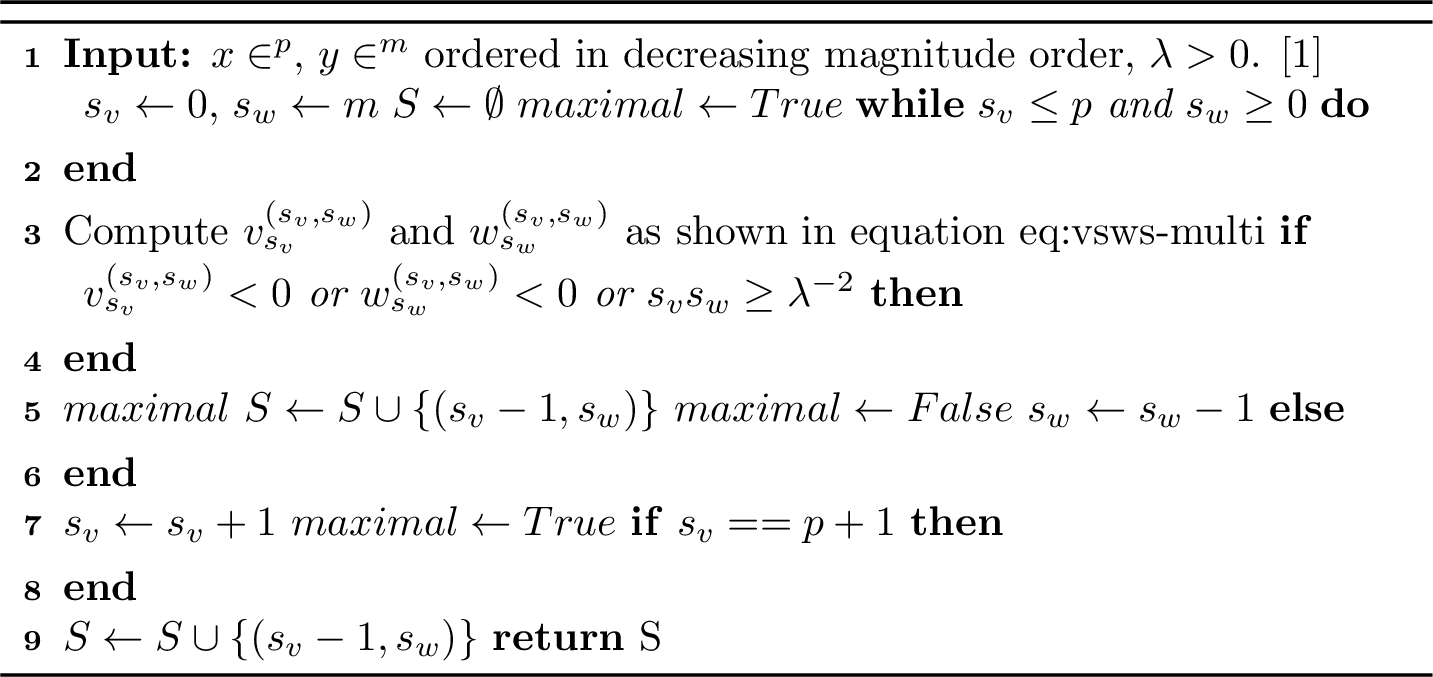
Lemma 18. The set \(S\) returned by Algorithm 5 contains all, and only, the sparsity pairs that are on the maximal feasibility boundary.
Proof. First recall that the MFB is defined as all pairs \((s_v,s_w) \in \{0,\ldots,p\} \times \{0,\ldots,m\}\) satisfying the conditions:
\(v^{(s_v, s_w)}_{s_v} > 0\) and \(w^{(s_v, s_w)}_{s_w} > 0\) and \(s_v s_w \leq \lambda^{-2}\),
\(v^{(s_v + 1, s_w)}_{s_v + 1} \leq 0\) or \(w^{(s_v + 1, s_w)}_{s_w} \leq 0\) or \((s_v+1)s_w > \lambda^{-2}\) or \(s_v = p\),
\(v^{(s_v, s_w+1)}_{s_v} \leq 0\) or \(w^{(s_v, s_w+1)}_{s_w+1} \leq 0\) or \(s_v(s_w+1) > \lambda^{-2}\) or \(s_w = m\).
Algorithm 5 plays on the properties of feasibility-infeasibility of the sparsity levels to build the MFB. We say that a pair of the sparsity levels of \(v\) and \(w\) \((s_v, s_w)\) is feasible if \(v_{s_v}^{(s_v, s_w)} \geq 0\), \(w_{s_w}^{(s_v, s_w)} \geq 0\) and \(s_v s_w < \lambda^{-2}\), and denote this by the property \(P(i, j)\), i.e. \[(i,j) \text{ is feasible } \Leftrightarrow P(i, j).\]
Our claim can be read as: Let \((i, j)\in \{0,\ldots,p\} \times \{0,\ldots,m\}\), then \((i, j)\) is added to \(S\) by Algorithm 5 if and only if \((i, j)\) belongs to the MFB, i.e., \[(i, j) \in \text{MFB} \Leftrightarrow (i, j) \in S.\] Obviously, only feasible sparsity pairs belong to the MFB, and it is quite easy to see that only feasible sparsity pairs will belong to an output \(S\) of Algorithm 5. Indeed, Algorithm 5 monotonically decrements \(s_w\) starting from \(s_w = m\) and increments \(s_v\) starting from \(s_v = 0\). For each value of \(s_w\), it increases \(s_v\) while the current pair \((s_v, s_w)\) is feasible (lines \(12-15\)). Once it reaches an infeasible point \((i,s_w)\), and in the case where \(s_v\) has been increased at least once for this particular value of \(s_w\), it adds to \(S\) the pair encountered just before, i.e., \((i-1, s_w)\), and then decrements \(s_w\) (lines \(6-11\)).
We first prove the \(\Rightarrow\) statement. Suppose that some pair \((i, j)\) belongs to the MFB. Let us first leave aside the corner cases, and assume that \(i < p\) and \(j < m\).
Suppose first that \(s_w\) reaches \(j\) before \(s_v\) reaches \(i\), i.e., \(s_v < i\). Since the pair \((i,j)\) is feasible, and due to the monotonicity property of the feasibility condition (Lemma 9), all pairs \((k,s_w)\) with \(k \leq i\) must be feasible. Therefore, \(s_v\) will be increased until reaching \(i+1\). By definition of the MFB, the pair \((i+1, j)\) must be infeasible. Since \(s_v\) has necessarily been increased at least once for this value of \(s_w=j\), and so the pair \((i+1-1, j) = (i,j)\) will be added to \(S\) before decrementing \(s_w\).
In the special case where \(i = p\), no infeasible point will be found. The loop will thus finish with \(s_w = j\) and \(s_v = p+1\). The condition at line \(17\) will thus hold, and the pair \((p,j)\) will be added to \(S\).
Suppose now that \(s_v\) reaches \(i\) before \(s_w\) reaches \(j\), i.e., \(s_w > j\). Since \((i,j)\) is in the MFB, then the pair \((i,j+1)\) must be infeasible. Thanks to the monotonicity property of the feasibility condition (Lemma 9), all pairs \((s_v,k)\) with \(k \geq i\) must also be infeasible. Therefore, \(s_w\) will be decreased until reaching \(s_w = j\). Then, similarly as in the previous case, since \((i,j)\) is feasible, \(s_v\) will be increased, and the pair \((i,j)\) added to \(S\).
We now prove the \(\Leftarrow\) statement. We show that if \((i,j)\) is added to \(S\), then it must belong to the MFB, i.e., it satisfies all three properties recalled in the beginning of the proof.
Let us first show that for each pair \((s_v, s_w)\) encountered during the algorithm, the pair \((s_v-1, s_w)\) is always feasible (or \(s_v = 0\)). We can show that this property is conserved each time the algorithm either increases \(s_v\) or decreases \(s_w\). First note that the pair \((0, m)\) is always feasible. The algorithm will then necessarily first goes to the pair \((1, m)\) and \(P(1,m)\) is true. Then suppose that \(P(s_v, s_w)\) is true for some pair \((s_v, s_w)\) encountered during the algorithm. Then, if \(s_v\) is increases, it means that the pair \((s_v, s_w)\) is feasible. The next encountered pair is then \((s_v+1, s_w)\) and \(P(s_v+1, s_w)\) is true. On the other hand, suppose that \(s_w\) is decreased. The next encountered pair is thus \((s_v, s_w-1)\). Since \(P(s_v, s_w)\) is true, it means that \((s_v-1, s_w)\) is feasible. By Lemma 9, it implies that \((s_v-1, s_w-1)\) is also feasible, and thus \(P(s_v, s_w-1)\) is true. We thus proved that \(P(s_v, s_w)\) is true for any pair \((s_v, s_w)\) encountered during the algorithm. Therefore, since any pair added to \(S\) is of the form \((s_v-1, s_w)\) for some pair \((s_v, s_w)\) encountered during the algorithm, then any pair added to \(S\) must be feasible.
The second property of the MFB is straightforward to show. Indeed, if \((i-1, j)\) is added to \(S\), it means that the pair \((i,j)\) is infeasible due to condition on line \(6\).
Finally, the third property follows from the fact that, when reaching \(s_w=j\), \(s_v\) must be increased at least once for adding a pair of the form \((i,j)\) to \(S\). Let \(s_v^{(j)}\) be the value of \(s_v\) when the algorithm reaches \(s_w = j\). We necessarily have \(s_v^{(j)} \leq i\). This implies that the pair \((s_v^{(j)}, j+1)\) is infeasible, otherwise \(s_v\) would have been increased to a greater value at the previous value \(s_w = j+1\). By Lemma 9, and since \(s_v^{(j)} \leq i\) this implies that the pair \((i,j+1)\) is also infeasible, hence the result.
The algorithm monotonically decrements \(s_w\) starting from \(s_w = m\) and increments \(s_v\) starting from \(s_v = 0\). For each value of \(s_w\), the algorithm increments \(s_v\) either \(0\) or multiple times. Let \(s_v^{(k)}\) be the first value of \(s_v\) immediately after \(s_w\) has been decremented to \(k\). Since \(s_v\) is never decreased and \(s_w\) is never increased, we have that \(0 = s_v^{(m)} \leq s_v^{(m-1)} \leq \ldots\). We also say that a pair \((s_v, s_w)\) is feasible if and only if \(v_{s_v}^{(s_v, s_w)} \geq 0\), \(w_{s_w}^{(s_v, s_w)} \geq 0\) and \(s_v s_w < \lambda^{-2}\).
For each \(k \in \{0,\ldots, m\}\), we will show by standard induction the property \(P(k)\): "For \(s_w = k\), then, if and only if there exists a pair \((s_v, k)\) for some \(s_v \in \{0, \ldots, p\}\) that belongs to the MFB, the algorithm will add this pair to \(S\)".
12.1.0.1 Initialization
Let us prove the result for \(k = m\). First note that for each value \(s_w\), \((0, s_w)\) is a feasible pair. Also note that there always exists a pair \((s_v, m)\) which belongs to the MFB for some value of \(s_v \in \{0, \ldots, p\}\). Indeed, there necessarily exists a feasible pair \((s_v, m)\) such that either \((s_v+1, m)\) is infeasible or \(s_v = p\), making such a pair belong to the MFB since the three conditions above would be satisfied. The algorithm starts from \(s_w=m\) and increments \(s_v\) until it finds a non feasible pair \((s_v, m)\). If it finds one, since the boolean \(maximal\) is initially set to \(True\), it adds to \(S\) the pair encountered just before, i.e., \((s_v-1, m)\), which is in the MFB by definition. If it does not find one, then the loop ends with \(s_v = p+1\), so that the condition of line \(15\) of the algorithm holds, and we thus add the pair \((p,m)\) (line \(16\) of the algorithm) which must then be in the MFB. Therefore, \(P(m)\) is true.
12.1.0.2 Recursion
Suppose that \(\exists k \in \{1,\ldots,m\}\) such that the property \(P(i)\) holds true for all \(i \in \{k,\ldots,m\}\), and let us prove that \(P(k-1)\) holds true as-well. First observe that each time \(s_w\) is decreased to \(k\), the boolean \(maximal\) is necessarily \(False\) because of the condition of line \(7\) of the algorithm which sets \(maximal\) to \(False\) (line \(10\)) if it was \(True\) before. Moreover, since each iteration ends at an infeasible pair, the pair \((s_v^{(k)}, k+1)\) is infeasible and the pair \((s_v^{(k)} -1,k+1)\) is feasible. The algorithm then again increments \(s_v\) until it finds a non feasible pair, giving three possible scenarios:
The current pair \((s_v^{k}, k)\) is already infeasible. In this case, \(s_v\) is not incremented and the boolean \(maximal\) remains \(False\). Thus, \(s_w\) is decremented, and no pair is added to \(S\). Moreover, since \((s_v^{(k)} -1,k+1)\) is feasible, and due to the monotonicity of the feasibility criterion, the pairs \((s,k)\) for \(s < s_v^{(k)} -1\) are not in the MFB. Moreover, the pairs \((s,k)\) for \(s \geq s_v^{(k)} -1\) are infeasible and thus not in the MFB. Thus, there exists no value of \(s_v \in \{0, \ldots, p\}\) such that the pair \((s_v, k)\) belongs to the MFB. So \(P(k-1)\) is true.
\(s_v\) is increased at least once and the algorithm finds a non feasible pair \((s_v^{(k+1)}, k)\) with \(s_v^{(k+1)} > s_v^{(k)}\). Since \(s_v\) has been increased, the boolean \(maximal\) is set to \(True\), and the pair \((s_v^{(k+1)}-1, k)\) is added to \(S\). Thanks to the monotonicity of the feasibility criterion, since \((s_v^{(k)}, k+1)\) is infeasible, then \((s_v^{(k+1)}-1, k+1)\) must also be infeasible. Therefore, since both \((s_v^{(k+1)}, k+1)\) and \((s_v^{(k+1)}, k)\), then \((s_v^{(k+1)}-1, k)\) belongs to the MFB, and this is indeed the pair that is added to \(S\). So \(P(k-1)\) is true.
The algorithm does not find any feasible point. Then again, the loop ends with \(s_v = p+1\), so that the condition of line \(17\) of the algorithm holds, and we thus add the pair \((p,m)\) (line \(18\) of the algorithm) which belongs to the MFB. Again, this implies that \(P(k-1)\) is true.
We thus proved that for each value of \(s_w\), the algorithm will add to \(S\) the unique pair \((s_v, s_w)\) for some \(s_v \in \{0, \ldots, p\}\) belonging to the MFB in the case where such a pair exists. Since the algorithm tests all values of \(s_w \in \{0, \ldots, m\}\), this proves the result. ◻
12.1.0.3 Time complexity of Algorithm 5
At each iteration of the loop, either \(s_v\) is incremented by \(1\) or \(s_w\) is decremented by \(1\). Since \(s_v\) starts from \(0\) and \(s_w\) from \(m\), and that the stopping criterion is \(s_v > p\) or \(s_w < 0\), it follows that the maximal number of iterations inside the loop is \(m+p\). At each iteration, we must compute \(v_{s_v}^{(s_v, s_w)}\) and \(w_{s_w}^{(s_v, s_w)}\), which requires in particular to compute \(\sum_{k=1}^{s_v} |x_k|\) and \(\sum_{j=1}^{s_w} |y_j|\). However, these cumulative sums can be efficiently computed before the loop in time \(\mathcal{O}(m+p)\), so that computing \(v_{s_v}^{(s_v, s_w)}\) and \(w_{s_w}^{(s_v, s_w)}\) inside the loop can be done in constant time. The overall complexity of this algorithm is thus \(\mathcal{O}(m+p)\).
Moreover, we can see that each time we add a pair to \(S\), we must both decrement \(s_w\) by \(1\) (just after adding the element in the algorithm), and increment \(s_v\) by \(1\) (in order for the boolean \(maximal\) to become true again). Therefore, there can be at most \(\min(m,p)\) pairs in the final set \(s\) at the end of the algorithm.
Merging all previous results, we can finally prove Theorem 4.
Proof of Theorem 4. Thanks to the separability argument, it is sufficient to prove that Algorithm 3 returns a solution of problem 8 .
Lemma 7 states that given the number of nonzero elements \(s_v = |\{k:v_k^* > 0\}|\), \(s_w = |\{j:w_j^* > 0\}|\), the optimal solution \((v^*, w^*)\) can be obtained in close form (equations ?? , ?? ).
Due the monotonicity property of the objective function \(h_\lambda\) (Lemma 9), it follows that the sparsity pair \((s_v, s_w)\) of the optimal solution must lie on the MFB. Indeed, if it does not lie on the MFB, then it means that the candidate solution associated with either the sparsity pair \((s_v+1, s_w)\) or \((s_v, s_w+1)\) must be feasible. According to Lemma 9, this pair would then yield a lower value of \(h_\lambda\), and would then be a better solution.
Algorithm 3 computes the candidate solution associated with all sparsity pair lying on the MFB, and returns the one achieving the lowest value of \(h_\lambda\). Therefore, the returned solution must necessarily be the optimal solution. ◻
13 Experimental details and other plots↩︎
We consider the following values for the parameters that determine the training loop:
batch size:
100epochs:
20learning rate:
1e-1, 1e-2, 1e-3, 1e-4, 5e-1, 5e-2, 5e-3, 5e-4dataset:
mnist, fmnist, kmnisthidden neurons:
200lambda (\(\lambda\)):
0., 1e-5, 1e-4, 1e-3, 1e-2, 1e-1, 1e0, 1e1, 1e2, 2e-5, 2e-4, 2e-3, 2e-2, 2e-1, 2e0, 2e1, 2e2, 3e-5, 3e-4, 3e-3, 3e-2, 3e-1, 3e0, 3e1, 3e2, 4e-5, 4e-4, 4e-3, 4e-2, 4e-1, 4e0, 4e1, 4e2, 5e-5, 5e-4, 5e-3, 5e-2, 5e-1, 5e0, 5e1, 5e2
The \(\ell_\infty\)-bounded adversarial examples used to evaluate the robustness of the networks were generated using the PGD method described in [3] and implemented in the advertorch toolbox (https://github.com/BorealisAI/advertorch) using the following parameters:
epsilon:
0.05, 0.1, 0.15, 0.2, 0.25, 0.3iterations: 40
step size: epsilon / 20
random initialization:
True
13.1 sparsity per iteration↩︎
One advantage of the proximal mapping of the 1-path-norm and the \(\ell_1\)-norm is that they can set many weights to exactly zero. This has the effect of providing sparse networks from early iterations. This is in contrast to SGD with a constant stepsize which does not generate sparse iterates. In Figures 4, 5, 6 and 7 we plot the percentage of nonzero weights as a function of the iteration count, for both plain SGD and proximal SGD. We observe that in fact this is the case, and that the sparsity of the \(\ell_1\) and 1-path-norm regularized network can be controlled with the regularization parameter \(\lambda\).

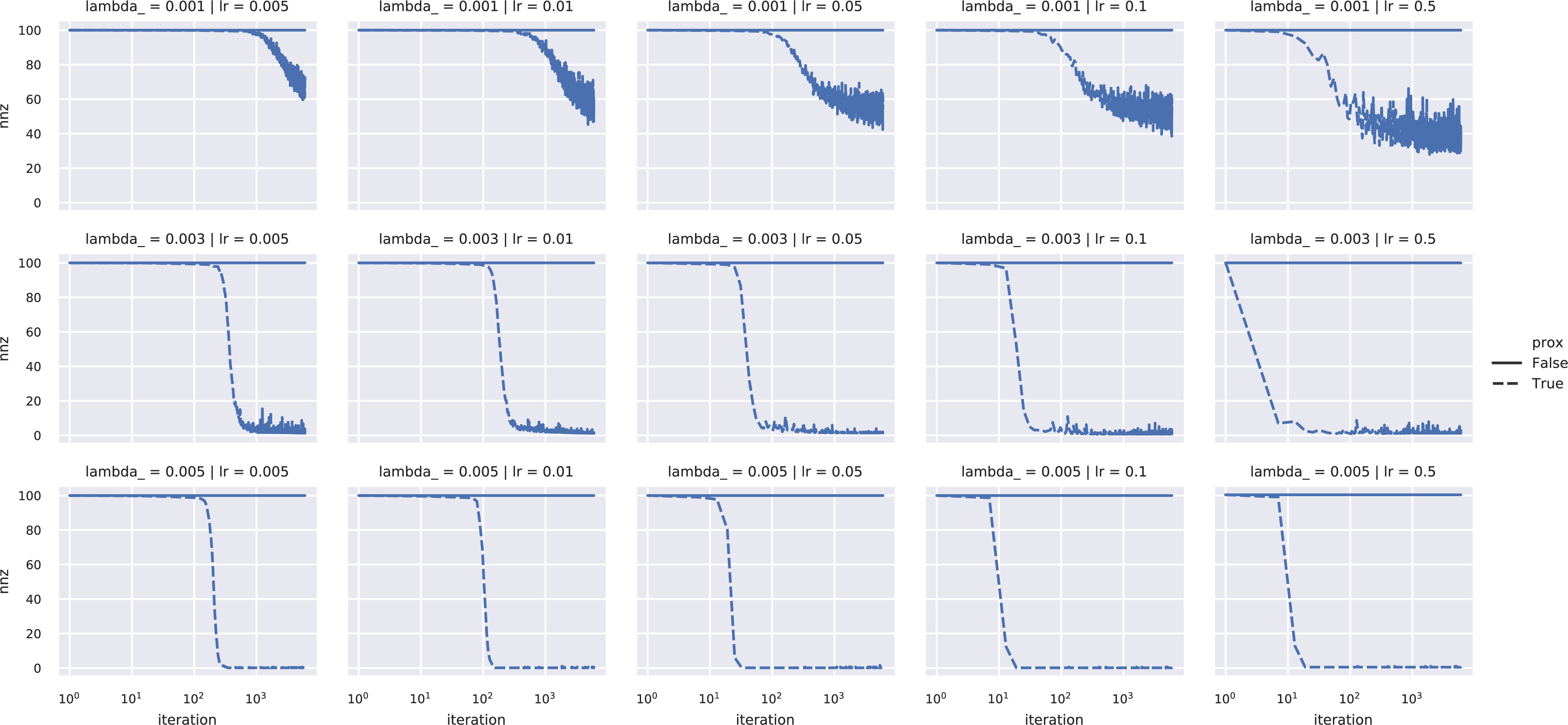
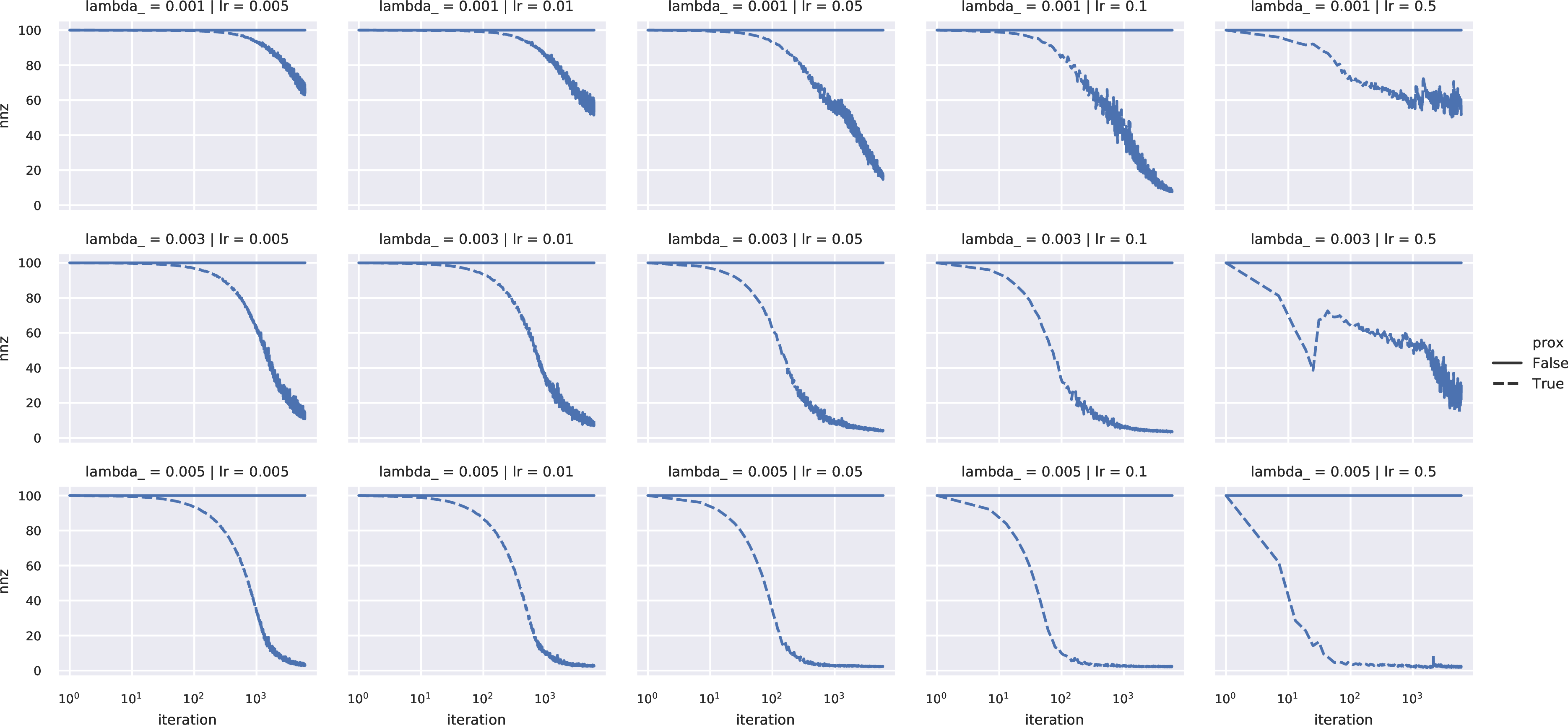
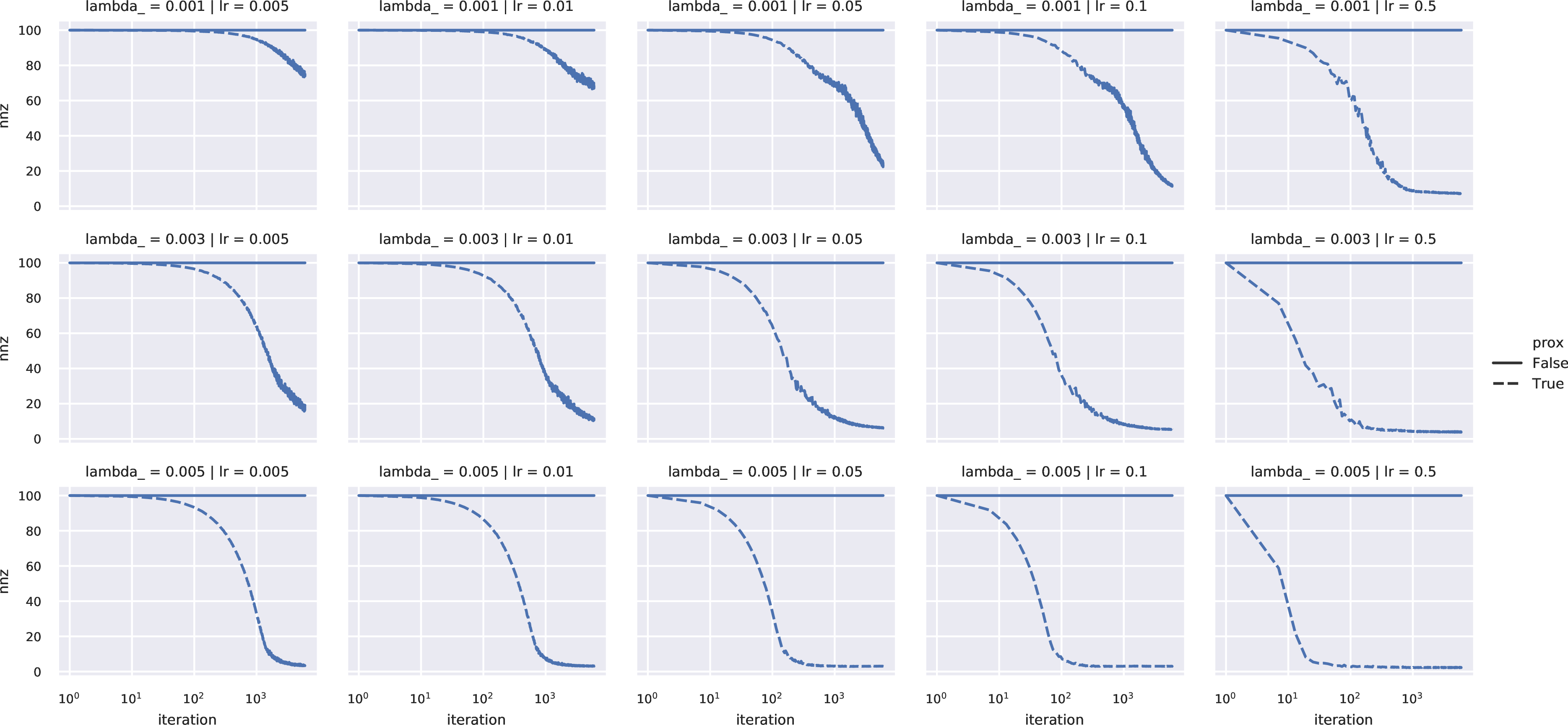
13.2 Robustness vs accuracy tradeoff↩︎
For all possible values of \(\lambda\), in Figure 8 we plot the data corresponding to the lerning rate with least error. We plot the value of the error on clean samples and the error on adversarial examples. This allows us to understand the tradeoff between accuracy and robustness that is controlled by the regularization paramter \(\lambda\).
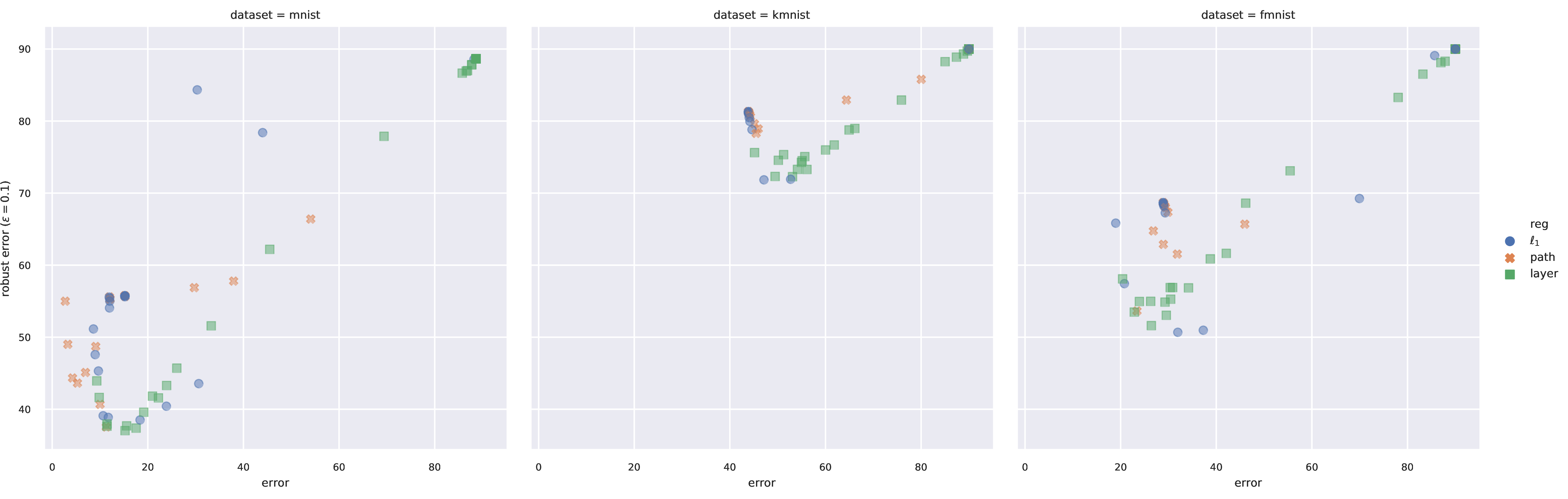
References↩︎
We will call an optimal solution trivial if \(v^* = 0\).↩︎