Adversarial Ranking Attack and Defense
February 26, 2020
Abstract
Deep Neural Network (DNN) classifiers are vulnerable to adversarial attack, where an imperceptible perturbation could result in misclassification. However, the vulnerability of DNN-based image ranking systems remains under-explored. In this paper, we propose two attacks against deep ranking systems, , Candidate Attack and Query Attack, that can raise or lower the rank of chosen candidates by adversarial perturbations. Specifically, the expected ranking order is first represented as a set of inequalities, and then a triplet-like objective function is designed to obtain the optimal perturbation. Conversely, a defense method is also proposed to improve the ranking system robustness, which can mitigate all the proposed attacks simultaneously. Our adversarial ranking attacks and defense are evaluated on datasets including MNIST, Fashion-MNIST, and Stanford-Online-Products. Experimental results demonstrate that a typical deep ranking system can be effectively compromised by our attacks. Meanwhile, the system robustness can be moderately improved with our defense. Furthermore, the transferable and universal properties of our adversary illustrate the possibility of realistic black-box attack.
1 Introduction↩︎
Despite the successful application in computer vision tasks such as image classification [1], [2], Deep Neural Networks (DNNs) have been found vulnerable to adversarial attacks. In particular, the DNN’s prediction can be arbitrarily changed by just applying an imperceptible perturbation to the input image [3], [4]. Moreover, such adversarial attacks can effectively compromise the recent state-of-the-art DNNs such as Inception [5], [6] and ResNet [2]. This poses a serious security risk on many DNN-based applications such as face recognition, where recognition evasion or impersonation can be easily achieved [7]–[10].
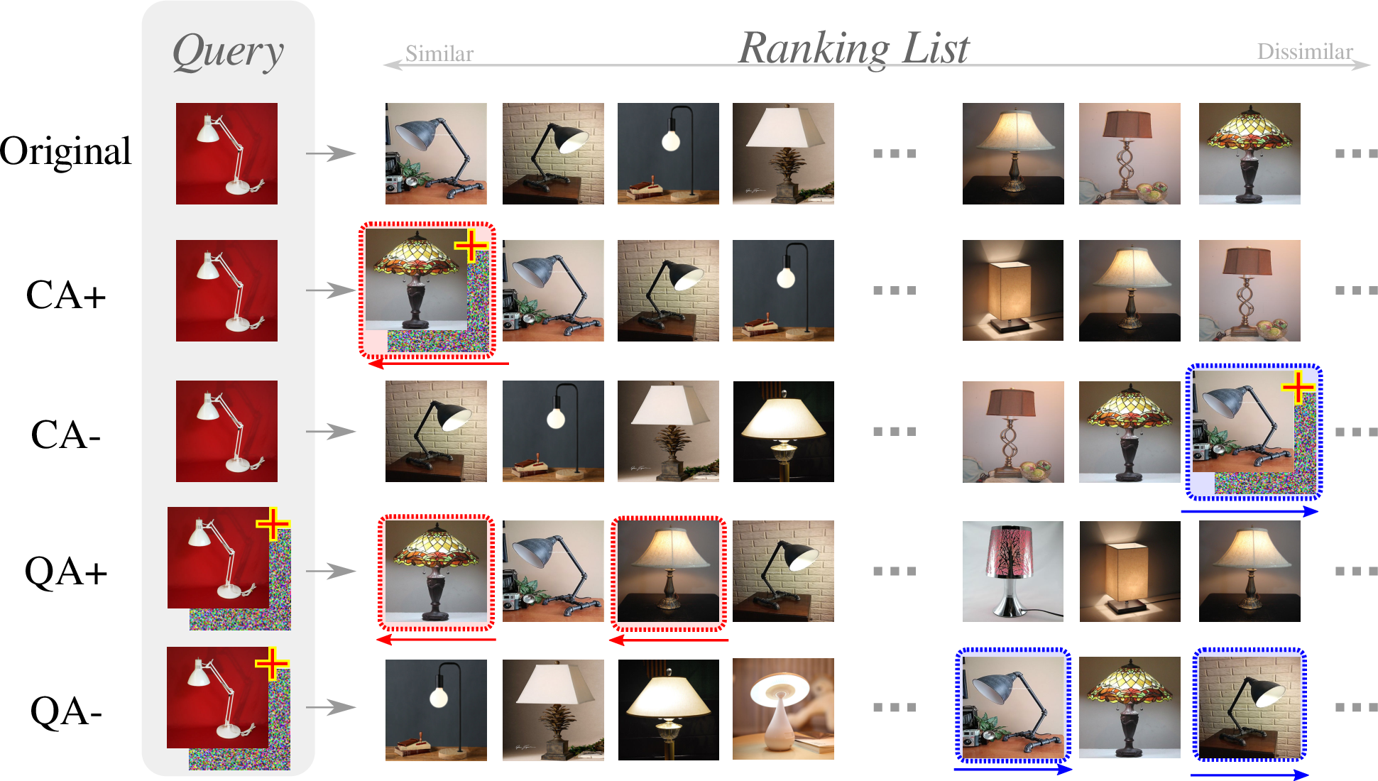
Previous adversarial attacks primarily focus on classification, however, we speculate that DNN-based image ranking systems [11]–[17] also suffer from similar vulnerability. Taking the image-based product search as an example, a fair ranking system should rank the database products according to their visual similarity to the query, as shown in Fig. 1 (row 1). Nevertheless, a malicious seller may attempt to raise the rank of his/her own product by adding perturbation to the image (CA+, row 2), or lower the rank of his competitor’s product (CA-, row 3); Besides, a “man-in-the-middle” attacker (., a malicious advertising company) could hijack and imperceptibly perturb the query image in order to promote (QA+, row 4) or impede (QA-, row 5) the sales of specific products.
Unlike classification tasks where images are predicted independently, the rank of one candidate is related to the query as well as other candidates for image ranking. The relative relations among candidates and queries determine the final ranking order. Therefore, we argue that the existing adversarial classification attacks are incompatible with the ranking scenario. Thus, we need to thoroughly study the adversarial ranking attack.
In this paper, adversarial ranking attack aims to raise or lower the ranks of some chosen candidates \(C=\{c_1,c_2,\ldots,c_m\}\) with respect to a specific query set \(Q=\{q_1,q_2,\ldots,q_w\}\). This can be achieved by either Candidate Attack (CA) or Query Attack (QA). In particular, CA is defined as to raise (abbr. CA+) or lower (abbr. CA-) the rank of a single candidate \(c\) with respect to the query set \(Q\) by perturbing \(c\) itself; while QA is defined as to raise (abbr. QA+) or lower (abbr. QA-) the ranks of a candidate set \(C\) with respect to a single query \(q\) by perturbing \(q\). Thus, adversarial ranking attack can be achieved by performing CA on each \(c\in C\), or QA on each \(q\in Q\). In practice, the choice of CA or QA depends on the accessibility to the candidate or query respectively, , CA is feasible for modifiable candidate, while QA is feasible for modifiable query.
An effective implementation of these attacks is proposed in this paper. As we know, a typical DNN-based ranking model maps objects (, queries and candidates) to a common embedding space, where the distances among them determine the final ranking order. Predictably, the object’s position in the embedding space will be changed by adding a perturbation to it. Therefore, the essential of adversarial ranking attack is to find a proper perturbation, which could push the object to a desired position that leads to the expected ranking order. Specifically, we first represent the expected ranking order as a set of inequalities. Subsequently, a triplet-like objective function is designed according to those inequalities, and combined with Projected Gradient Descent (PGD) to efficiently obtain the desired adversarial perturbation.
Opposed to the proposed attacks, adversarial ranking defense is worth being investigated especially for security-sensitive deep ranking applications. Until now, the Madry defense [18] is regarded as the most effective method for classification defense. However, we empirically discovered a primary challenge of diverging training loss while directly adapting such mechanism for ranking defense, possibly due to the generated adversarial examples being too “strong”. In addition, such defense mechanism needs to defend against distinct ranking attacks individually, but a generic defense method against all CA+, CA-, QA+ and QA- attacks is preferred.
To this end, a shift-distance based ranking defense is proposed, which could simultaneously defend against all attacks. Note that the position shift of objects in the embedding space is the key for all ranking attacks. Although different attacks prefer distinct shift directions (, CA+ and CA- often prefer opposed shifting directions), a large shift distance is their common preference. If we could reduce the shift distance of embeddings incurred by adversarial perturbation, all attacks can be simultaneously defensed. Specifically, we first propose a shift-distance based ranking attack, which aims to push the objects as far from their original positions as possible. And then, the adversarial examples generated from such attack is involved in the adversarial training. Experimental results manifest that our ranking defense can converge and moderately improve model robustness.
In addition, our ranking attacks have some good properties for realistic applications. First, our adversary is transferable, , the adversary obtained from a known DNN ranker can be directly used to attack an unknown DNN ranker (, the network architecture and parameters are unknown). Second, our attacks can be extended to universal ranking attacks with slight performance drop, , we could learn a universal perturbation to all candidates for CA, or a universal perturbation to all queries for QA. Such properties illustrate the possibility of practical black-box attack.
To the best of our knowledge, this is the first work that thoroughly studies the adversarial ranking attack and defense. In brief, our contributions are:
The adversarial ranking attack is defined and implemented, which can intentionally change the ranking results by perturbing the candidates or queries.
An adversarial ranking defense method is proposed to improve the ranking model robustness, and mitigate all the proposed attacks simultaneously.
2 Related Works↩︎
Adversarial Attacks. Szegedy [3] claimed that DNN is susceptible to imperceptible adversarial perturbations added to inputs, due to the intriguing “blind spot” property, which was later ascribed to the local linearity [4] of neural networks. Following these findings, many white-box (model architecture and parameters are known to the adversary) attacking methods [18]–[29] are proposed to effectively compromise the state-of-the-art DNN classifiers. Among them, PGD [18] is regarded as one of the most powerful attacks [30]. Notably, adversarial examples are discovered to be transferable [31], [32] among different neural network classifiers, which inspired a series of black-box attacks [33]–[38]. On the other hand, universal (, image-agnostic) adversarial perturbations are also discovered [39], [40]. The existence of adversarial examples stimulated research interests in areas such as object detection [41]–[43], semantic segmentation [44], and automatic speech recognition [45], . It is even possible to create physical adversarial examples [8], [10], [46], [47].
Deep Ranking. Different from the traditional “learning to rank” [48], [49] methods, DNN-based ranking methods often embed data samples (including both queries and candidates) of all modalities into a common embedding space, and subsequently determine the ranking order based on distance. Such workflow has been adopted in distance metric learning [12], [13], [50], [51], image retrieval [11], cross-modal retrieval [14]–[17], and face recognition [52].
Adversarial Attacks in Deep Ranking. For information retrieval and ranking systems, the risk of malicious users manipulating the ranking always exists [53], [54]. However, only a few research efforts have been made in adversarial attacks in deep ranking. Liu [55] proposed adversarial queries leading to incorrect retrieval results; while Li [56] staged similar attack with universal perturbation that corrupts listwise ranking results. None of the aforementioned research efforts explore the adversarial ranking attack. Besides, adaptation of distance-based attacks ( [25]) are unsuitable for our scenario.
Adversarial Defenses. Adversarial attacks and defenses are consistently engaged in an arms race [57]. Gradient masking-based defenses can be circumvented [58]. Defensive distillation [59], [60] has been compromised by C&W [22], [61]. As claimed in [62], ensemble of weak defenses are insufficient against adversarial examples. Notably, as an early defense method [3], adversarial training [4], [18], [63]–[69] remains to be one of the most effective defenses. Other types of defenses include adversarial detection [70], [71], input transformation/reconstruction/replacement [72]–[76], randomization [77], [78], feature denoising [79], network verification [80], [81], evidential deep learning [82], . However, defense in deep ranking systems remains mostly uncharted.
3 Adversarial Ranking↩︎
Generally, a DNN-based ranking task could be formulated as a metric learning problem. Given the query \(q\) and candidate set \(X=\{c_1,c_2,\ldots,c_n\}\), deep ranking is to learn a mapping \(f\) (usually implemented as a DNN) which maps all candidates and query into a common embedding space, such that the relative distances among the embedding vectors could satisfy the expected ranking order. For instance, if candidate \(c_i\) is more similar to the query \(q\) than candidate \(c_j\), it is encouraged for the mapping \(f\) to satisfy the inequality \(\|f(q)-f(c_i)\|<\|f(q)-f(c_j)\|\)1, where \(\|\cdot\|\) denotes \(\ell_2\) norm. For brevity, we denote \(\|f(q)-f(c_i)\|\) as \(d(q,c_i)\) in following text.
Therefore, adversarial ranking attack is to find a proper adversarial perturbation which leads the ranking order to be changed as expected. For example, if a less relevant \(c_j\) is expected to be ranked ahead of a relevant \(c_i\), it is desired to find a proper perturbation \(r\) to perturb \(c_j\), \(\tilde{c}_j=c_j+r\), such that the inequality \(d(q,c_i)<d(q,c_j)\) could be changed into \(d(q,c_i)>d(q,\tilde{c}_j)\). In the next, we will describe Candidate Attack and Query Attack in detail.
3.1 Candidate Attack↩︎
Candidate Attack (CA) aims to raise (abbr. CA+) or lower (abbr. CA-) the rank of a single candidate \(c\) with respect to a set of queries \(Q=\{q_1,q_2,\ldots,q_w\}\) by adding perturbation \(r\) to the candidate itself, \(\tilde{c}=c+r\).
Let \(\text{Rank}_X(q,c)\) denote the rank of the candidate \(c\) with respect to the query \(q\), where \(X\) indicates the set of all candidates, and a smaller rank value represents a higher ranking. Thus, the CA+ that raises the rank of \(c\) with respect to every query \(q\in Q\) by perturbation \(r\) could be formulated as the following problem, \[\begin{align} r &= \mathop{\mathrm{arg\,min}}_{r\in\Gamma}\sum_{q\in Q}\text{Rank}_X(q,c+r), \tag{1} \\ \Gamma &= \{r \big| \|r\|_\infty\leqslant\varepsilon; r,c+r\in [0,1]^N \}, \tag{2} \end{align}\] where \(\Gamma\) is a \(\ell_\infty\)-bounded \(\varepsilon\)-neighbor of \(c\), \(\varepsilon \in [0,1]\) is a predefined small positive constant, the constraint \(\|r\|_\infty \leqslant \varepsilon\) limits the perturbation \(r\) to be “visually imperceptible”, and \(c+r\in [0,1]^N\) ensures the adversarial example remains a valid input image. Although alternative “imperceptible” constraints exist (, \(\ell_0\) [26], [83], \(\ell_1\) [23] and \(\ell_2\) [19], [22] variants), we simply follow [4], [18], [21] and use the \(\ell_\infty\) constraint.
However, the optimization problem Eq. 1 –2 cannot be directly solved due to the discrete nature of the rank value \(\text{Rank}_X(q,c)\). In order to solve the problem, a surrogate objective function is needed.
In metric learning, given two candidates \(c_p, c_n \in X\) where \(c_p\) is ranked ahead of \(c_n\), \(\text{Rank}_X(q,c_p) < \text{Rank}_X(q,c_n)\), the ranking order is represented as an inequality \(d(q,c_p)<d(q,c_n)\) and formulated in triplet loss: \[L_{\text{triplet}}(q,c_p,c_n)=\left[\beta + d(q,c_p) - d(q,c_n)\right]_+, \label{eq:triplet}\tag{3}\] where \([\cdot]_+\) denotes \(\max(0,\cdot)\), and \(\beta\) is a manually defined constant margin. This function is known as the triplet (pairwise ranking) loss [12], [52].
Similarly, the attacking goal of CA+ in Eq. 1 can be readily converted into a series of inequalities, and subsequently turned into a sum of triplet losses, \[L_{\text{CA+}}(c,Q;X)=\sum_{q\in Q}\sum_{x\in X}\big[d(q,c)-d(q,x)\big]_{+}. \label{eq:ca4395loss}\tag{4}\] In this way, the original problem in Eq. 1 –2 can be reformulated into the following constrained optimization problem: \[r=\mathop{\mathrm{arg\,min}}_{r\in\Gamma}L_{\text{CA+}}(c+r,Q;X). \label{eq:ca95opt}\tag{5}\]
To solve the optimization problem, Projected Gradient Descent (PGD) method [18], [21] (a.k.a the iterative version of FGSM [4]) can be used. Note that PGD is one of the most effective first-order gradient-based algorithms [30], popular among related works about adversarial attack.
Specifically, in order to find an adversarial perturbation \(r\) to create a desired adversarial candidate \(\tilde{c}=c+r\), the PGD algorithm alternates two steps at every iteration \(t=1, 2,\ldots,\eta\). Step one updates \(\tilde{c}\) according to the gradient of Eq. 4 ; while step two clips the result of step one to fit in the \(\varepsilon\)-neighboring region \(\Gamma\): \[\tilde{c}_{t+1}=\text{Clip}_{c,\Gamma}\big\{\tilde{c}_{t} -\alpha\text{sign}(\nabla_{\tilde{c}_t}L_{\text{CA+}}(\tilde{c}_t,Q,X))\big\}, \label{eq:PGDsteps}\tag{6}\] where \(\alpha\) is a constant hyper-parameter indicating the PGD step size, and \(\tilde{c}_1\) is initialized as \(c\). After \(\eta\) iterations, the desired adversarial candidate \(\tilde{c}\) is obtained as \(\tilde{c}_{\eta}\), which is optimized to satisfy as many inequalities as possible. Each inequality represents a pairwise ranking sub-problem, hence the adversarial candidate \(\tilde{c}\) will be ranked ahead of other candidates with respect to every specified query \(q\in Q\).
Likewise, the CA- that lowers the rank of a candidate \(c\) with respect to a set of queries \(Q\) can be obtained in similar way: \[L_{\text{CA-}}(c,Q;X)=\sum_{q\in Q}\sum_{x\in X}\big[-d(q,c)+d(q,x)\big]_{+}. \label{eq:ca-95loss}\tag{7}\]
3.2 Query Attack↩︎
Query Attack (QA) is supposed to raise (abbr. QA+) or lower (abbr. QA-) the rank of a set of candidates \(C=\{c_1,c_2,\ldots,c_m\}\) with respect to the query \(q\), by adding adversarial perturbation \(r\) to the query \(\tilde{q}=q+r\). Thus, QA and CA are two “symmetric” attacks. The QA- for lowering the rank could be formulated as follows: \[r=\mathop{\mathrm{arg\,max}}_{r\in\Gamma}\sum_{c\in C}\text{Rank}_X(q+r,c), \label{eq:qa95intuitive}\tag{8}\] where \(\Gamma\) is the \(\varepsilon\)-neighbor of \(q\). Likewise, this attacking objective can also be transformed into the following constrained optimization problem: \[\begin{align} L_{\text{QA-}}(q,C;X)&=\sum_{c\in C}\sum_{x\in X}\big[-d(q,c)+d(q,x)\big]_{+}, \tag{9}\\ r&=\mathop{\mathrm{arg\,min}}_{r\in\Gamma}L_{\text{QA-}}(q+r,C;X), \tag{10} \end{align}\] and it can be solved with the PGD algorithm. Similarly, the QA+ loss function \(L_{\text{QA+}}\) for raising the rank of \(c\) is as follows: \[L_{\text{QA+}}(q,C;X)=\sum_{c\in C}\sum_{x\in X}\big[d(q,c)-d(q,x)\big]_{+}. \label{eq:qa43}\tag{11}\]
Unlike CA, QA perturbs the query image, and hence may drastically change its semantics, resulting in abnormal retrieval results. For instance, after perturbing a “lamp” query image, some unrelated candidates (, “shelf”, “toaster”, ) may appear in the top return list. Thus, an ideal query attack should preserve the query semantics, , the candidates in \(X \setminus C\) 2 should retain their original ranks if possible. Thus, we propose the Semantics-Preserving Query Attack (SP-QA) by adding the SP term to mitigate the semantic changes \(q\), ,
\[L_{\text{SP-QA-}}(q,C;X)=L_{\text{QA-}}(q,C;X) + \xi L_{\text{QA+}}(q,C_{\text{SP}};X), \label{eq:spqa}\tag{12}\]
where \(C_{\text{SP}} = \left\{ c \in X \setminus C | \text{Rank}_{X \setminus C}(q,c) \leqslant G \right\}\), , \(C_{\text{SP}}\) contains the top-\(G\) most-relevant candidates corresponding to \(q\), and the \(L_{\text{QA+}}(q,C_{\text{SP}};X)\) term helps preserve the query semantics by retaining some \(C_{\text{SP}}\) candidates in the retrieved ranking list. Constant \(G\) is a predefined integer; and constant \(\xi\) is a hyper-parameter for balancing the attack effect and semantics preservation. Unless mentioned, in the following text QA means SP-QA by default.
3.3 Robustness & Defense↩︎
Adversarial defense for classification has been extensively explored, and many of them follows the adversarial training mechanism [18], [63], [65]. In particular, the adversarial counterparts of the original training samples are used to replace or augment the training samples. Until now, Madry defense [18] is regarded as the most effective [58], [67] adversarial training method. However, when directly adapting such classification defense to improve ranking robustness, we empirically discovered a primary challenge of diverging training loss, possibly due to the generated adversarial examples being too “strong”. Moreover, such defense mechanism needs to defend against distinct attacks individually. Therefore, a generic defense against all the proposed attacks is preferred.
Note that the underlying principle of adversarial ranking attack is to shift the embeddings of candidates/queries to a proper place, and a successful attack depends on a large shift distance as well as a correct shift direction. A large shift distance is an indispensable objective for all the CA+, CA-, QA+ and QA- attacks. Predictably, a reduction in shift distance could improve model robustness against all attacks simultaneously.
To this end, we propose a “maximum-shift-distance” attack that pushes an embedding vector as far from its original position as possible (resembles Feature Adversary [25] for classification), \(r = \mathop{\mathrm{arg\,max}}_{r\in\Gamma} d(c+r, c) \label{eq:es}\). Then we use adversarial examples obtained from this attack to replace original training samples for adversarial training, hence reduce the shift distance incurred by adversarial perturbations.
A ranking model can be normally trained with the defensive version of the triplet loss:
\[\begin{align} L_{\text{d-t}}(q,c_p,c_n) = L_{\text{triplet}} \Big( & q + \mathop{\mathrm{arg\,max}}_{r\in\Gamma}d(q+r,q),\nonumber \\ & c_p + \mathop{\mathrm{arg\,max}}_{r\in\Gamma}d(c_p+r,c_p),\nonumber \\ & c_n + \mathop{\mathrm{arg\,max}}_{r\in\Gamma}d(c_n+r,c_n) \Big). \label{eq:defense} \end{align}\tag{13}\]
Unlike the direct adaptation of Madry defense, the training loss does converge in our experiments.
4 Experiments↩︎
| \(\varepsilon\) | CA+ | CA- | QA+ | QA- | ||||||||||||
| \(w=1\) | \(2\) | \(5\) | \(10\) | \(w=1\) | \(2\) | \(5\) | \(10\) | \(m=1\) | \(2\) | \(5\) | \(10\) | \(m=1\) | \(2\) | \(5\) | \(10\) | |
| 0 | 50 | 50 | 50 | 50 | 2.1 | 2.1 | 2.1 | 2.1 | 50 | 50 | 50 | 50 | 0.5 | 0.5 | 0.5 | 0.5 |
| 0.01 | 44.6 | 45.4 | 47.4 | 47.9 | 3.4 | 3.2 | 3.1 | 3.1 | 45.2 | 46.3 | 47.7 | 48.5 | 0.9 | 0.7 | 0.6 | 0.6 |
| 0.03 | 33.4 | 37.3 | 41.9 | 43.9 | 6.3 | 5.9 | 5.7 | 5.6 | 35.6 | 39.2 | 43.4 | 45.8 | 1.9 | 1.4 | 1.1 | 1.1 |
| 0.1 | 12.7 | 17.4 | 24.4 | 30.0 | 15.4 | 14.9 | 14.8 | 14.7 | 14.4 | 21.0 | 30.6 | 37.2 | 5.6 | 4.4 | 3.7 | 3.5 |
| 0.3 | 2.1 | 9.1 | 13.0 | 17.9 | 93.9 | 93.2 | 93.0 | 92.9 | 6.3 | 11.2 | 22.5 | 32.1 | 8.6 | 6.6 | 5.3 | 4.8 |
To validate the proposed attacks and defense, we use three commonly used ranking datasets including MNIST [84], Fashion-MNIST [85], and Stanford Online Product (SOP) [50]. We respectively train models on these datasets with PyTorch [86], and conduct attacks 3 on their corresponding test datasets (used as \(X\)).
Evaluation Metric. Adversarial ranking attack aims to change the ranks of candidates. For each candidate \(c\), its normalized rank is calculated as \(R(q,c) = \frac{\text{Rank}_X(q,c)}{|X|}\times 100\%\) where \(c\in X\), and \(|X|\) is the length of full ranking list. Thus, \(R(q,c)\in [0,1]\), and a top ranked \(c\) will have a small \(R(q,c)\). The attack effectiveness can be measured by the magnitude of change in \(R(q,c)\).
Performance of Attack. To measure the performance of a single CA attack, we average the rank of candidate \(c\) across every query \(q \in Q\), , \(R_\text{CA}(c)=\sum_{q\in Q}{R}(q,c)/w\). Similarly, the performance of a single QA attack can be measured by the average rank across every candidate \(c \in C\), , \(R_\text{QA}(q)=\sum_{c\in C}{R}(q,c)/m\). For the overall performance of an attack, we conduct \(T\) times of independent attacks and report the mean of \(R_\text{CA}(c)\) or \(R_\text{QA}(q)\), accordingly.
CA+ & QA+. For CA+, the query set \(Q\) is randomly sampled from \(X\). Likewise, for QA+, the candidate set \(C\) is from \(X\). Without attack, both the \(R_\text{CA}(c)\) and \(R_\text{QA}(q)\) will approximate to \(50\%\), and the attacks should significantly decrease the value.
CA- & QA-. In practice, the \(Q\) for CA- and the \(C\) for QA- cannot be randomly sampled, because the two attacks are often to lower some top ranked candidates. Thus, the two sets should be selected from the top ranked samples (top-\(1\%\) in our experiments) in \(X\). Formally, given the candidate \(c\) for CA-, we randomly sample the \(w\) queries from \(\left\{ q \in X | R(c,q) \leqslant 1\% \right\}\) as \(Q\). Given the query \(q\) for QA-, \(m\) candidates are randomly sampled from \(\left\{ c \in X | R(q,c) \leqslant 1\% \right\}\) as \(C\). Without attack, both the \(R_\text{CA}(c)\) and \(R_\text{QA}(q)\) will be close to \(0\%\), and the attacks should significantly increase the value.
Hyper-Parameters. We conduct CA with \(w \in \{1,2,5,10\}\) queries, and QA with \(m \in \{1,2,5,10\}\) candidates, respectively. In QA, we let \(G=5\). The SP balancing parameter \(\xi\) is set to \(1\) for QA+ , and \(10^2\) for QA-. In addition, We investigate attacks of different strength \(\varepsilon\), \(0.01,0.03,0.1,0.3\) on MNIST and Fashion-MNIST following [18], and \(0.01,0.03,0.06\) on SOP following [65]. The PGD step size is empirically set to \(\alpha=\min(\max(\frac{\varepsilon}{10},\frac{1}{255}),0.01)\), and the number of PGD iterations to \(\eta=\min(\max(10, \frac{2\varepsilon}{\alpha}),30)\). We perform \(T=|X|\) times of attack to obtain the reported performance.
Adversarial Defense. Ranking models are trained using Eq. 13 with the strongest adversary following the procedure of Madry defense [18].
4.1 MNIST Dataset↩︎
| \(\varepsilon\) | CA+ | CA- | QA+ | QA- | ||||||||||||
| \(w=1\) | \(2\) | \(5\) | \(10\) | \(w=1\) | \(2\) | \(5\) | \(10\) | \(m=1\) | \(2\) | \(5\) | \(10\) | \(m=1\) | \(2\) | \(5\) | \(10\) | |
| 0 | 50 | 50 | 50 | 50 | 2.0 | 2.0 | 2.0 | 2.0 | 50 | 50 | 50 | 50 | 0.5 | 0.5 | 0.5 | 0.5 |
| 0.01 | 48.9 | 49.3 | 49.4 | 49.5 | 2.2 | 2.2 | 2.2 | 2.1 | 49.9 | 49.5 | 49.5 | 49.7 | 0.5 | 0.5 | 0.5 | 0.5 |
| 0.03 | 47.4 | 48.4 | 48.6 | 48.9 | 2.5 | 2.5 | 2.4 | 2.4 | 48.0 | 48.5 | 49.2 | 49.5 | 0.6 | 0.6 | 0.5 | 0.5 |
| 0.1 | 42.4 | 44.2 | 45.9 | 46.7 | 3.8 | 3.6 | 3.5 | 3.4 | 43.2 | 45.0 | 47.4 | 48.2 | 1.0 | 0.8 | 0.7 | 0.7 |
| 0.3 | 30.7 | 34.5 | 38.7 | 40.7 | 7.0 | 6.7 | 6.5 | 6.5 | 33.2 | 37.2 | 42.3 | 45.1 | 2.4 | 1.9 | 1.6 | 1.5 |
Following conventional settings with the MNIST [84] dataset, we train a CNN ranking model comprising \(2\) convolutional layers and \(1\) fully-connected layer. This CNN architecture (denoted as C2F1) is identical to the one used in [18] except for the removal of the last fully-connected layer. Specifically, the ranking model is trained with cosine distance and triplet loss. The retrieval performance of the model is Recall@1=\(99.1\%\) (R@\(1\)), as shown in Tab. 1 in grey highlight.
Attacking results against this vanilla model (, the ranking model which is not enhanced with our defense method) are presented in Tab. 1. For example, a strong CA+ attack (, \(\varepsilon=0.3\)) for \(w=1\) can raise the rank \(R_\text{CA}(c)\) from \(50\%\) to \(2.1\%\). Likewise, the rank of \(C\) can be raised to \(9.1\%\), \(13.0\%\), \(17.9\%\) for \(w=2,5,10\) chosen queries, respectively.
On the other hand, a strong CA- attack for \(w=1\) can lower the rank \(R_\text{CA}(c)\) from \(2.1\%\) to \(93.9\%\). The results of strong CA- attacks for \(w=2,5,10\) are similar to the \(w=1\) case.
The results of QA+ and QA- are also shown in Tab. 1. the rank changes with QA attacks are less dramatic (but still significant) than CA. This is due to the additional difficulty introduced by SP term in Eq. 12 , and the QA attack effectiveness is inversely correlated with \(\xi\). For instance, a strong QA- for \(m=1\) can only lower the rank \(R_\text{QA}(q)\) from \(0.5\%\) to \(8.6\%\), but the attacking effect can be further boosted by decreasing \(\xi\). More experimental results are presented in following discussion. In brief, our proposed attacks against the vanilla ranking model is effective.
Next, we evaluate the performance of our defense method. Our defense should be able to enhance the robustness of a ranking model, which can be measured by the difference between the attack effectiveness with our defense and the attack effectiveness without our defense. As a common phenomenon of adversarial training, our defense mechanism leads to a slight retrieval performance degradation for unperturbed input (highlighted in blue in Tab. 2), but the attacking effectiveness is clearly mitigated by our defense. For instance, the same strong CA+ attack for \(w=1\) on the defensive model (, the ranking model which is enhanced by our defense method) can only raise the rank \(R_\text{CA}(c)\) from \(50\%\) to \(30.7\%\), compared to its vanilla counterpart raising to \(2.1\%\). Further analysis suggests that the weights in the first convolution layer of the defensive model are closer to \(0\) and have smaller variance than those of the vanilla model, which may help resist adversarial perturbation from changing the layer outputs into the local linear area of ReLU [4].
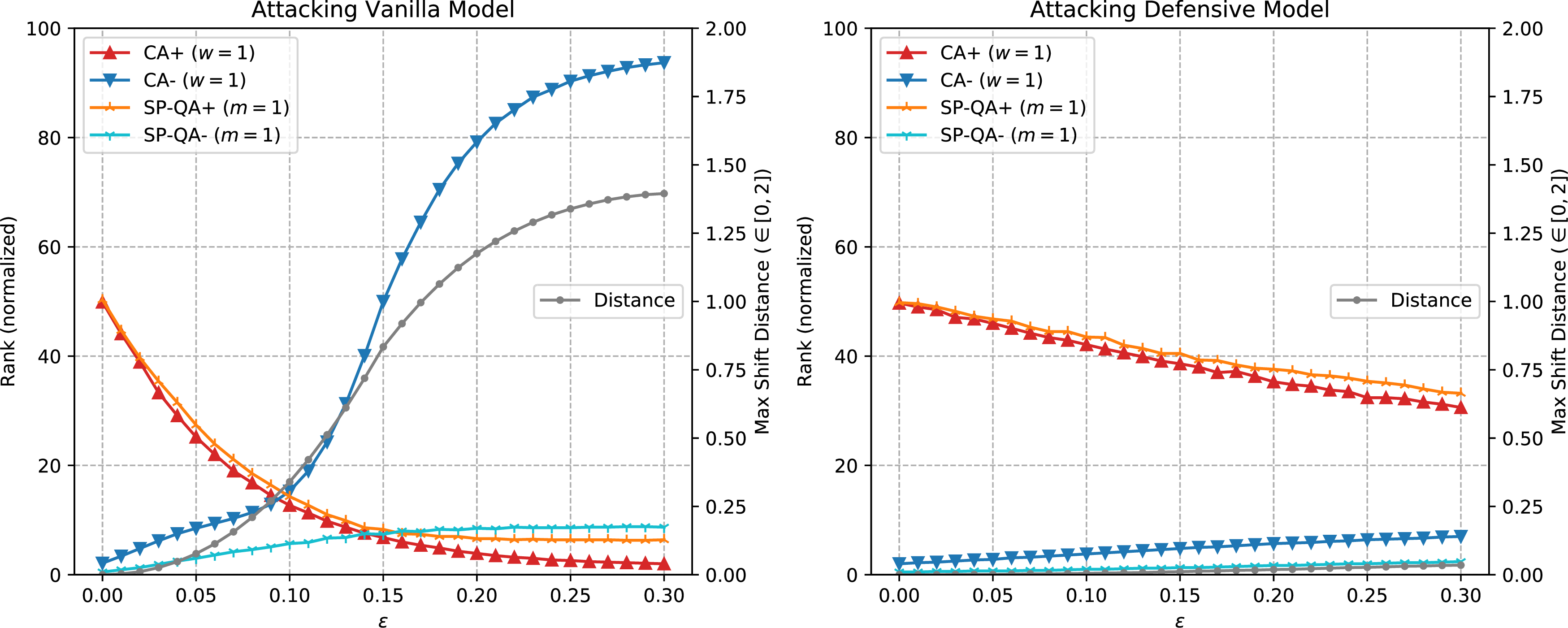
To visualize the effect of our attacks and defense, we track the attacking effect with \(\varepsilon\) varying from \(0.0\) to \(0.3\) on the vanilla and defensive models, as shown in Fig. 2. It is noted that our defense could significantly suppress the maximum embedding shift distance incurred by adversarial perturbation to nearly \(0\), but the defensive model is still not completely immune to attacks. We speculate the defensive model still has “blind spots” [3] in some local areas that could be exploited by the attacks.
In summary, these results and further experiments suggest that: (1) deep ranking models are vulnerable to adversarial ranking attacks, no matter what loss function or distance metric is selected; (2) vanilla models trained with contrastive loss are more robust than those trained with triplet loss. This is possibly due to contrastive loss explicitly reducing the intra-class embedding variation. Additionally, our defense method could consistently improve the robustness of all these models; (3) different distance metrics have almost negligible contribution on robustness. Specifically, Euclidean distance-based models are slightly more susceptible to weak (, \(\varepsilon=0.03\)) attacks; (4) Euclidean distance-based models are harder to defend than cosine distance-based ones. Beyond these experiments, we also find that the margin hyper-parameter \(\beta\) of triplet loss and the dimensionality of the embedding space have marginal influences on model robustness.
4.2 Fashion-MNIST Dataset↩︎
| \(\varepsilon\) | CA+ | CA- | QA+ | QA- | ||||||||||||
| \(w=1\) | \(2\) | \(5\) | \(10\) | \(w=1\) | \(2\) | \(5\) | \(10\) | \(m=1\) | \(2\) | \(5\) | \(10\) | \(m=1\) | \(2\) | \(5\) | \(10\) | |
| 0 | 50 | 50 | 50 | 50 | 1.9 | 1.9 | 1.9 | 1.9 | 50 | 50 | 50 | 50 | 0.5 | 0.5 | 0.5 | 0.5 |
| 0.01 | 36.6 | 39.9 | 43.2 | 44.8 | 5.6 | 5.1 | 4.9 | 4.8 | 39.4 | 42.0 | 45.3 | 47.1 | 2.1 | 1.6 | 1.2 | 1.1 |
| 0.03 | 19.7 | 25.4 | 31.7 | 35.6 | 15.5 | 14.8 | 14.4 | 14.3 | 21.7 | 28.2 | 35.7 | 40.6 | 5.6 | 4.1 | 3.3 | 2.9 |
| 0.1 | 3.7 | 10.5 | 17.3 | 22.7 | 87.2 | 86.7 | 86.3 | 86.3 | 7.1 | 12.4 | 23.6 | 32.5 | 10.9 | 8.3 | 6.7 | 6.0 |
| 0.3 | 1.3 | 9.4 | 16.0 | 21.5 | 100.0 | 100.0 | 100.0 | 100.0 | 6.3 | 10.8 | 21.8 | 31.7 | 12.6 | 9.4 | 7.5 | 6.6 |
| 0 | 50 | 50 | 50 | 50 | 1.2 | 1.2 | 1.2 | 1.2 | 50 | 50 | 50 | 50 | 0.5 | 0.5 | 0.5 | 0.5 |
| 0.01 | 48.9 | 48.9 | 49.3 | 49.3 | 1.4 | 1.4 | 1.4 | 1.4 | 49.4 | 49.9 | 49.9 | 50.0 | 0.5 | 0.5 | 0.5 | 0.5 |
| 0.03 | 47.1 | 47.9 | 48.3 | 48.3 | 2.0 | 1.9 | 1.8 | 1.8 | 48.3 | 49.1 | 49.5 | 49.8 | 0.7 | 0.6 | 0.6 | 0.6 |
| 0.1 | 42.4 | 43.5 | 44.5 | 44.8 | 4.6 | 4.2 | 4.0 | 3.9 | 45.4 | 47.2 | 48.7 | 49.2 | 1.4 | 1.2 | 1.1 | 1.1 |
| 0.3 | 32.5 | 35.4 | 37.5 | 38.2 | 11.2 | 10.5 | 10.1 | 10.0 | 39.3 | 42.6 | 46.5 | 47.8 | 3.9 | 3.3 | 3.0 | 2.9 |
0.2em
Fashion-MNIST [85] is an MNIST-like but more difficult dataset, comprising \(60,000\) training examples and \(10,000\) test samples. The samples are \(28\times 28\) greyscale images covering \(10\) different fashion product classes, including “T-shirt” and “dress”, . We train the vanilla and defensive models based on the cosine distance and triplet loss and conduct attack experiments.
The attack and defense results are available in Tab. 3. From the table, we note that our attacks could achieve better effect compared to experiments on MNIST. For example, in a strong CA+ for \(w=1\), the rank \(R_\text{CA}(c)\) can be raised to \(1.3\%\). On the other hand, despite the moderate improvement in robustness, the defensive model performs worse in unperturbed sample retrieval, as expected. The performance degradation is more pronounced on this dataset compared to MNIST. We speculate the differences are related to the increased dataset difficulty.
4.3 Stanford Online Products Dataset↩︎
Stanford Online Products (SOP) dataset [50] contains \(120\)k images of \(23\)k classes of real online products from eBay for metric learning. We use the same dataset split as used in the original work [50]. We also train the same vanilla ranking model using the same triplet ranking loss function with Euclidean distance, except that the GoogLeNet [5] is replaced with ResNet-18 [2]. The ResNet-18 achieves better retrieval performance.
Attack and defense results on SOP are present in Tab. 4. It is noted that our attacks are quite effective on this difficult large-scale dataset, as merely \(1\%\) perturbation (\(\varepsilon=0.01\)) to any candidate image could make it ranked ahead or behind of nearly all the rest candidates (as shown by the CA+ and CA- results with \(w=1\)). The QA on this dataset is significantly effective as well. On the other hand, our defense method leads to decreased retrieval performance, i.e. R@1 from \(63.1\%\) to \(46.4\%\), which is expected on such a difficult dataset. Meanwhile, our defense could moderately improve the model robustness against relatively weaker adversarial examples (e.g. \(\varepsilon=0.01\)), but improving model robustness on this dataset is more difficult, compared to experiments on other datasets.
By comparing the results among all the three datasets, we find ranking models trained on harder datasets more susceptible to adversarial attack, and more difficult to defend. Therefore, we speculate that models used in realistic applications could be easier to attack, because they are usually trained on larger-scale and more difficult datasets.
| \(\varepsilon\) | CA+ | CA- | QA+ | QA- | ||||||||||||
| \(w=1\) | \(2\) | \(5\) | \(10\) | \(w=1\) | \(2\) | \(5\) | \(10\) | \(m=1\) | \(2\) | \(5\) | \(10\) | \(m=1\) | \(2\) | \(5\) | \(10\) | |
| 0 | 50 | 50 | 50 | 50 | 1.9 | 1.9 | 1.9 | 1.9 | 50 | 50 | 50 | 50 | 0.5 | 0.5 | 0.5 | 0.5 |
| 0.01 | 0.0 | 0.8 | 2.0 | 2.6 | 99.7 | 99.6 | 99.4 | 99.3 | 4.8 | 7.0 | 16.3 | 25.8 | 54.9 | 40.2 | 27.1 | 21.9 |
| 0.03 | 0.0 | 0.3 | 1.0 | 1.5 | 100.0 | 100.0 | 100.0 | 100.0 | 1.6 | 3.3 | 10.0 | 19.2 | 68.1 | 52.4 | 36.6 | 30.1 |
| 0.06 | 0.0 | 0.2 | 1.0 | 1.5 | 100.0 | 100.0 | 100.0 | 100.0 | 1.1 | 2.7 | 8.8 | 17.6 | 73.8 | 57.9 | 40.3 | 32.4 |
| 0 | 50 | 50 | 50 | 50 | 2.0 | 2.0 | 2.0 | 2.0 | 50 | 50 | 50 | 50 | 0.5 | 0.5 | 0.5 | 0.5 |
| 0.01 | 7.5 | 12.2 | 16.5 | 18.0 | 66.4 | 62.6 | 59.3 | 57.8 | 16.1 | 24.8 | 36.1 | 41.4 | 26.7 | 18.1 | 12.2 | 10.2 |
| 0.03 | 0.7 | 4.5 | 8.7 | 10.4 | 91.7 | 90.2 | 89.1 | 88.4 | 7.9 | 14.5 | 27.2 | 35.6 | 43.4 | 31.7 | 21.9 | 18.1 |
| 0.06 | 0.1 | 3.8 | 7.9 | 9.7 | 97.3 | 96.8 | 96.4 | 96.2 | 6.9 | 12.5 | 24.3 | 33.4 | 51.4 | 39.0 | 28.0 | 23.5 |
0.2em
5 Discussions↩︎
In this section, we study the transferability of our adversarial ranking examples, and universal adversarial perturbation for ranking. Both of them illustrate the possibility of practical black-box attack. Additionally, we also perform parameter search on the balancing parameter \(\xi\) for QA.
5.1 Adversarial Example Transferability↩︎
As demonstrated in previous experiments, deep ranking models can be compromised by our white-box attacks. In realistic scenarios, the white-box attacks are not practical enough because the model to be attacked is often unknown (, the architecture and parameters are unknown).
On the other hand, adversarial examples for classification have been found transferable [31], [32] (model-agnostic) between different models with different network architectures. And the transferability has become the foundation of a class of existing black-box attacks. Specifically, for such a typical attack, adversarial examples are generated from a replacement model [31] using a white-box attack, and are directly used to attack the black-box model.
Adversarial ranking attack could be more practical if the adversarial ranking examples have the similar transferability. Besides the C2F1 model, we train two vanilla models on the MNIST dataset: (1) LeNet [84], which has lower model capacity compared to C2F1; (2) ResNet-18 [2] (denoted as Res18), which has a better network architecture and higher model capacity.
| LeNet | C2F1 | Res18 | |
| LeNet | 50\(\rightarrow\)16.6 | 35.1 | 34.3 |
| C2F1 | 28.6 | 50\(\rightarrow\)2.1 | 31.3 |
| Res18 | 24.4 | 27.0 | 50\(\rightarrow\)2.2 |
| LeNet | C2F1 | Res18 | |
| LeNet | 2.5\(\rightarrow\)63.7 | 2.1\(\rightarrow\)10.0 | 2.1\(\rightarrow\)9.1 |
| C2F1 | 2.5\(\rightarrow\)9.1 | 2.1\(\rightarrow\)93.9 | 2.1\(\rightarrow\)9.3 |
| Res18 | 2.5\(\rightarrow\)9.9 | 2.1\(\rightarrow\)11.8 | 2.1\(\rightarrow\)66.7 |
| LeNet | C2F1 | Res18 | |
| LeNet | 50\(\rightarrow\)20.5 | 43.0 | 45.8 |
| C2F1 | 43.5 | 50\(\rightarrow\)6.3 | 45.4 |
| Res18 | 41.4 | 40.4 | 50\(\rightarrow\)14.1 |
| LeNet | C2F1 | Res18 | |
| LeNet | 0.5\(\rightarrow\)7.0 | 0.5\(\rightarrow\)1.6 | 0.5\(\rightarrow\)1.8 |
| C2F1 | 0.5\(\rightarrow\)1.0 | 0.5\(\rightarrow\)8.6 | 0.5\(\rightarrow\)1.9 |
| Res18 | 0.5\(\rightarrow\)0.8 | 0.5\(\rightarrow\)1.2 | 0.5\(\rightarrow\)6.9 |
0.2em
The results are present in Tab. ¿tbl:tab:transfer?. For example, in the CA+ transfer attack, we generate adversarial candidates from the C2F1 model and directly use them to attack the Res18 model (row 2, column 3, top-left table), and the ranks of the adversarial candidates with respect to the same query is still raised to \(31.3\%\). We also find the CA- transfer attack is effective, where the ranks of our adversarial candidates are lowered, e.g. from \(2.1\%\) to \(9.3\%\) (row 2, column 3, bottom-left table). Similar results can be observed on the QA transfer experiments, and they show weaker effect due to the SP term.
From the results, we find that: (1) CNN with better architecture and higher model capacity (, Res18) is less susceptible to adversarial ranking attack. This conclusion is consistent with Madry’s [18], which claims that higher model capacity could help improve model robustness; (2) adversarial examples generated from the Res18 have the most significant effectiveness in transfer attack; (3) CNN of low model capacity (, LeNet), performs moderately in terms of both adversarial example transferability and model robustness. We speculate its robustness stems from a forced regularization effect due low model capacity. Beyond these, adversarial ranking examples are transferable disregarding the difference in loss function or distance metric.
Apart from transferability across different architectures, we also investigated the transferability between the C2F1 models with different network parameters. Results suggest similar transferability between these models. Notably, when transferring adversarial examples to a defensive C2F1 model, the attacking effect is significantly mitigated. The result further demonstrates the effectiveness of our defense.
5.2 Universal Perturbation for Ranking↩︎
Recently, universal (image-agnostic) adversarial perturbation [39] for classification has been found possible, where a single perturbation may lead to misclassification when added to any image. Thus, we also investigate the existence of universal adversarial perturbation for ranking.
To this end, we follow [39] and formulate the image-agnostic CA+ (abbr. I-CA+). Given a set of candidates \(C=\{c_1,c_2,\ldots,c_m\}\) and a set of queries \(Q=\{q_1,q_2,\ldots,q_w\}\), I-CA+ is to find a single universal adversarial perturbation \(r\), so that the rank of every perturbed candidate \(\tilde{c}=c+r ~ (c\in C)\) with respect to \(Q\) can be raised. The corresponding optimization problem of I-CA+ is: \[r=\mathop{\mathrm{arg\,min}}_{r\in\Gamma} \sum_{c\in C} L_\text{CA+}(c+r,Q;X).\] When applied with such universal perturbation, the rank of any candidate w.r.t \(Q\) is expected to be raised. The objective functions of I-CA-, I-QA+ and I-QA- can be obtained in similar way. Note, unlike [56] which aims to find universal perturbation that can make image retrieval system return irrelevant results, our universal perturbations have distinct purposes.
We conduct experiment on the MNIST dataset. For I-CA+ attack, we randomly sample \(5\%\) of \(X\) for generating the universal perturbation. Following [39], another non-overlapping \(5\%\) examples are randomly sampled from \(X\) to test whether the generated perturbation is generalizable on “unseen” (, not used for generating the perturbation) images. Experiments for the other image-agnostic attacks are conducted similarly. Note, we only report the I-CA- and I-QA- effectiveness on the \(1\%\) top ranked samples, similar to CA- and QA-.
| CA+ | CA- | QA+ | QA- |
| 50 \(\rightarrow\) 2.1 | 2.1 \(\rightarrow\) 93.9 | 50 \(\rightarrow\) 0.2 | 0.5 \(\rightarrow\) 94.1 |
| I-CA+ | I-CA- | I-QA+ | I-QA- |
| 50 \(\rightarrow\) 18.1 | 0.6 \(\rightarrow\) 9.5 | 50 \(\rightarrow\) 20.5 | 2.1 \(\rightarrow\) 7.6 |
| I-CA+ (unseen) | I-CA- (unseen) | I-QA+ (unseen) | I-QA- (unseen) |
| 50 \(\rightarrow\) 18.5 | 0.7 \(\rightarrow\) 9.4 | 50 \(\rightarrow\) 21.0 | 2.2 \(\rightarrow\) 7.4 |
0.4em
As shown in Tab. 5, our I-CA can raise the ranks of \(C\) to \(18.1\%\), or lower them to \(9.5\%\). When added to “unseen” candidate images, our universal perturbation could retain nearly the same effectiveness. This may due to low intra-class variance of the MNIST dataset.
5.3 Semantics Preserving for QA↩︎
As discussed previously, the Query Attack (QA) may drastically change the semantics of the query \(q\). To alleviate this problem, the Semantics-Preserving (SP) term is added to the naive QA to help preserve the query semantics. Predictably, it is more difficult to perform QA with a large \(\xi\), as the ranks of \(C_\text{SP}\) are almost not allowed to be changed.
To investigate the actual influence of the balancing parameter \(\xi\), we provide parameter search on it with MNIST dataset. In particular, We set \(\xi\) to \(0,10^0,10^2,10^4\), and compare their results. Note that when \(\xi=0\), the QA becomes naive QA as the SP term is eliminated. With a strong SP constant, \(\xi=10^4\), the semantics of the chosen query is almost not allowed to be changed, hence result in extreme difficulty of attack.
As shown in Tab. 6, setting \(\xi\) to \(0\) could greatly boost the attacking effect, but consequently the ranks of \(C_\text{SP}\) will be drastically changed. In contrast, when \(\xi\) is set to the excessive value \(10^4\) for a perfectly stealth QA, the attack can still raise the rank of chosen candidate from \(50\%\) to \(37.9\%\) in QA+ with \(m=1\), or lower the rank of chosen candidate from \(0.5\%\) to \(1.9\%\) in QA- with \(m=1\). During these attacks, the ranks of \(C_\text{SP}\) are kept within \(0.1\) despite of the extreme difficulty. It means the query semantics can be preserved. In practice, we empirically set the parameter \(\xi\) as \(1\) for QA+, or as \(10^2\) for QA- for the balance between attack effectiveness and preserving query semantics.
| \(\xi\) | QA+ | QA- | ||||||
| m=1 | 2 | 5 | 10 | m=1 | 2 | 5 | 10 | |
| 0 | 0.2, 33.6 | 6.3, 23.7 | 18.5, 26.5 | 29.6, 25.7 | 94.1, 89.4 | 93.2, 90.3 | 92.6, 90.9 | 92.3, 91.2 |
| \(10^0\) | 6.3, 3.6 | 11.2, 5.7 | 22.5, 7.7 | 32.1, 7.7 | 55.5, 35.6 | 52.4, 37.6 | 50.2, 39.3 | 49.4, 40.0 |
| \(10^2\) | 14.1, 0.6 | 20.8, 0.7 | 31.2, 0.7 | 38.1, 0.7 | 8.6, 1.6 | 6.6, 1.6 | 5.3, 1.5 | 4.8, 1.5 |
| \(10^4\) | 37.9, 0.1 | 42.6, 0.1 | 46.3, 0.1 | 47.8, 0.1 | 1.9, 0.1 | 1.4, 0.1 | 1.2, 0.1 | 1.1, 0.1 |
0.2em
6 Conclusion↩︎
Deep ranking models are vulnerable to adversarial perturbations that could intentionally change the ranking result. In this paper, we define and implement adversarial ranking attack that can compromise deep ranking models. We also propose an adversarial ranking defense that can significantly suppress embedding shift distance and moderately improve the ranking model robustness. Moreover, the transferability of our adversarial examples and the existence of universal adversarial perturbations for ranking attack illustrate the possibility of practical black-box attack and potential risk of realistic ranking applications. In the potential of future work, we may explore better ranking loss functions, defenses, and black-box attacks.
Acknowledgements↩︎
This work was supported partly by National Key R&D Program of China Grant 2018AAA0101400, NSFC Grants 61629301, 61773312, 61976171, and 61672402, China Postdoctoral Science Foundation Grant 2019M653642, Young Elite Scientists Sponsorship Program by CAST Grant 2018QNRC001, and Natural Science Foundation of Shaanxi Grant 2020JQ-069.
7 Adversarial Example Visualization↩︎
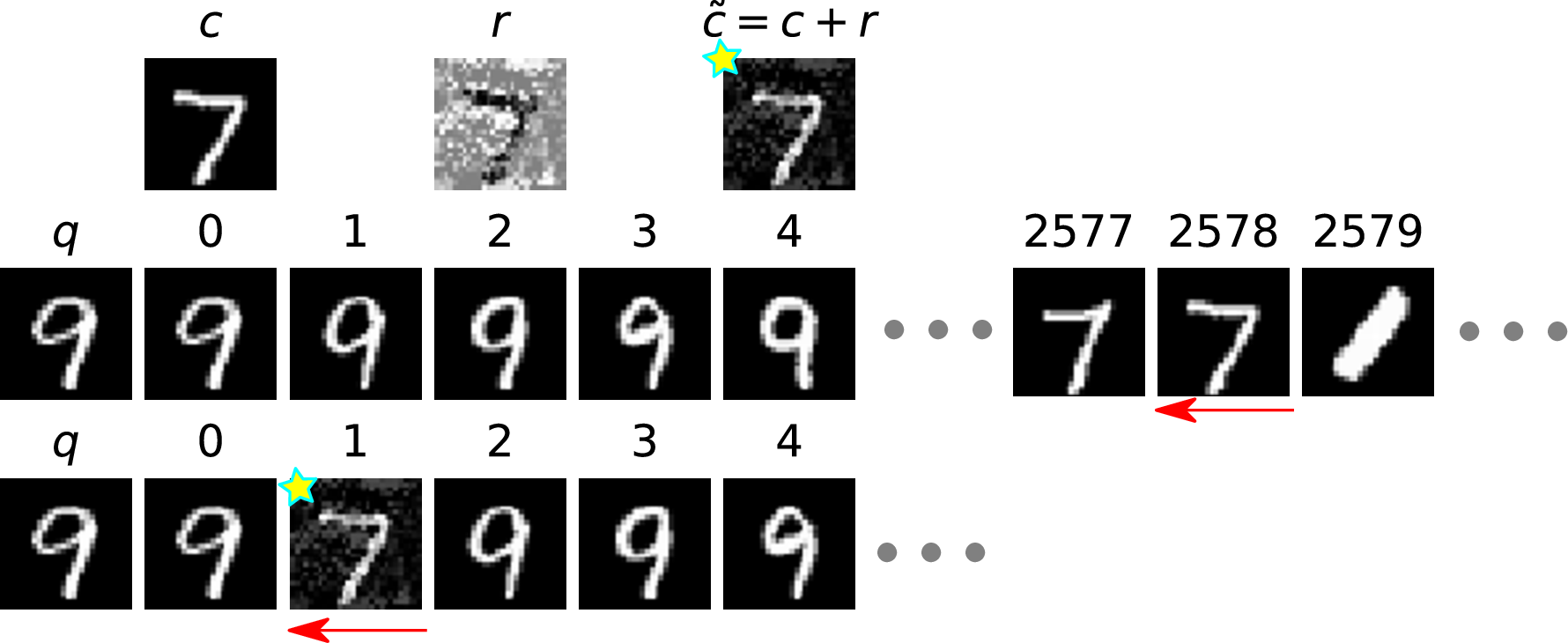
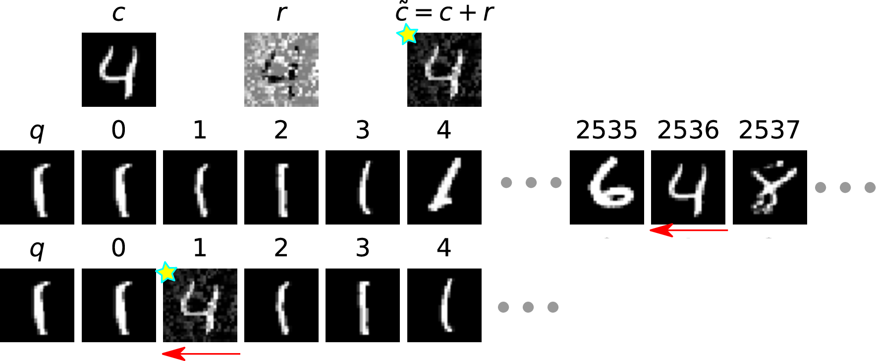
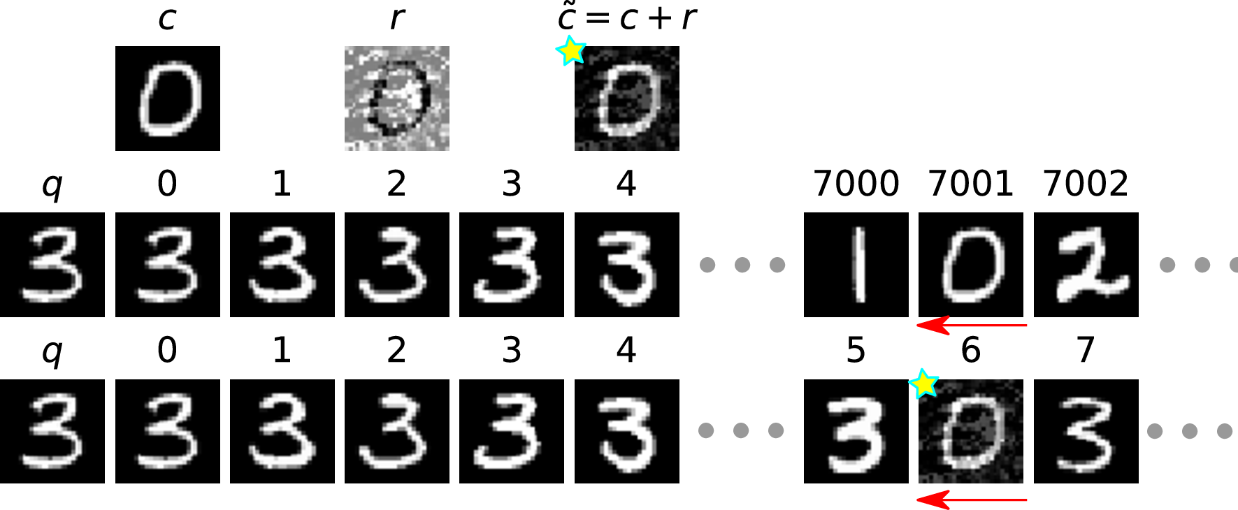
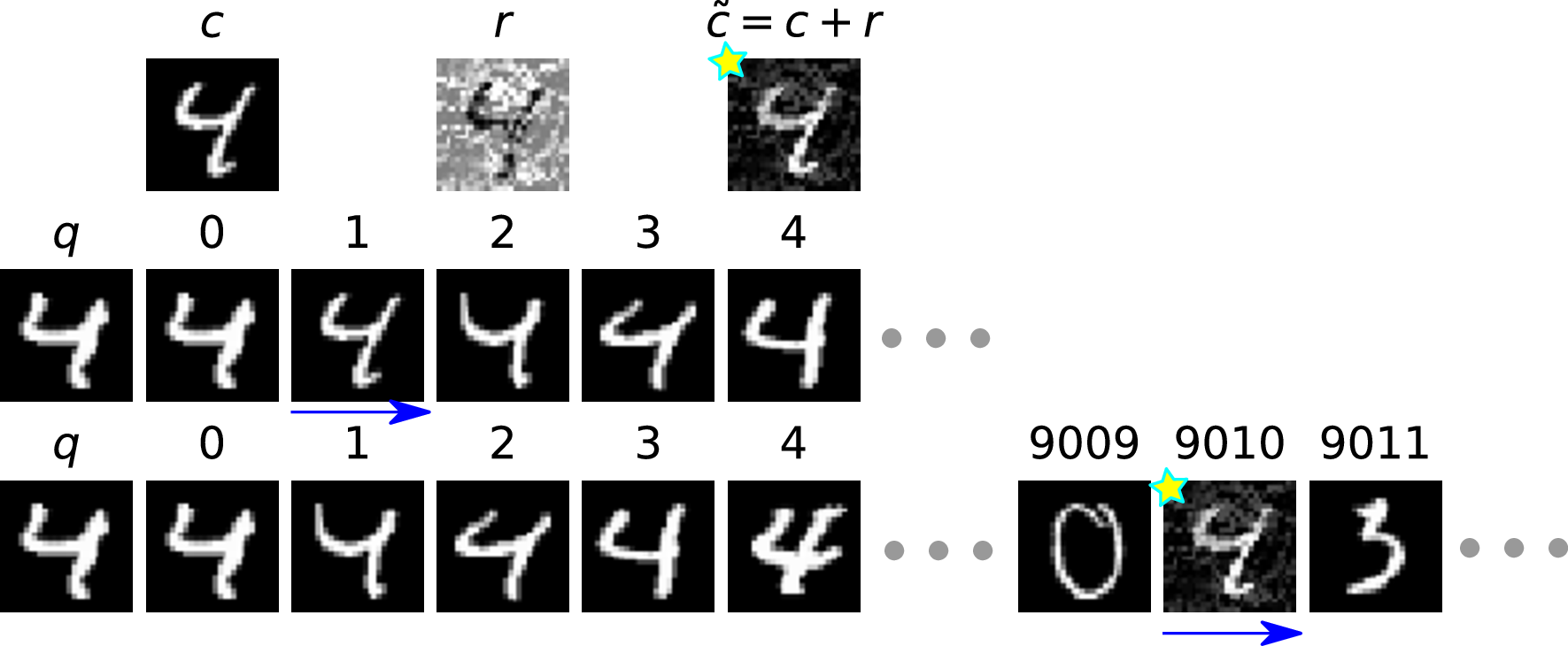
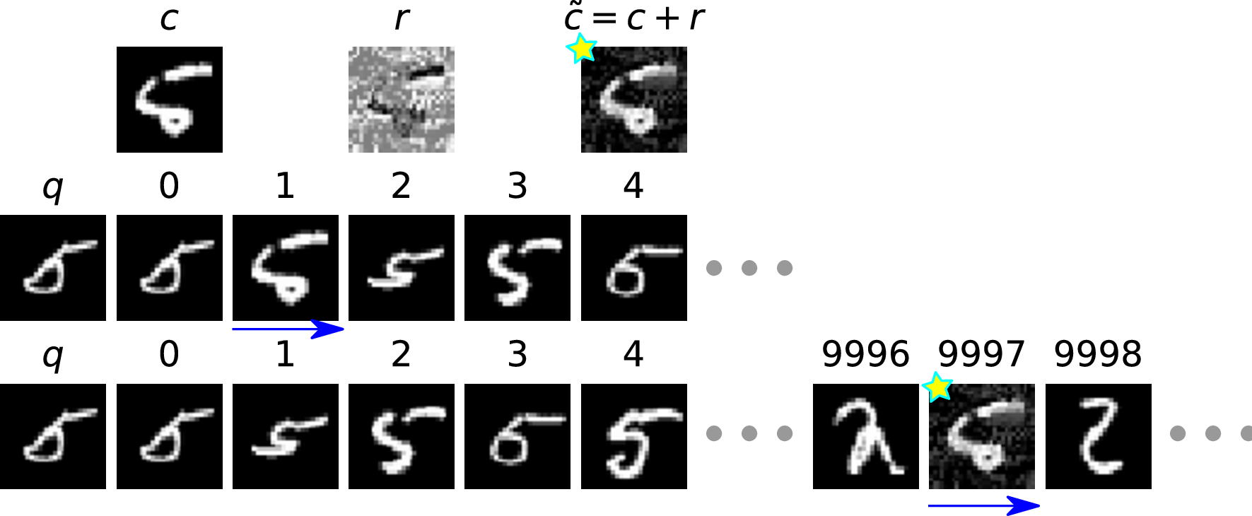
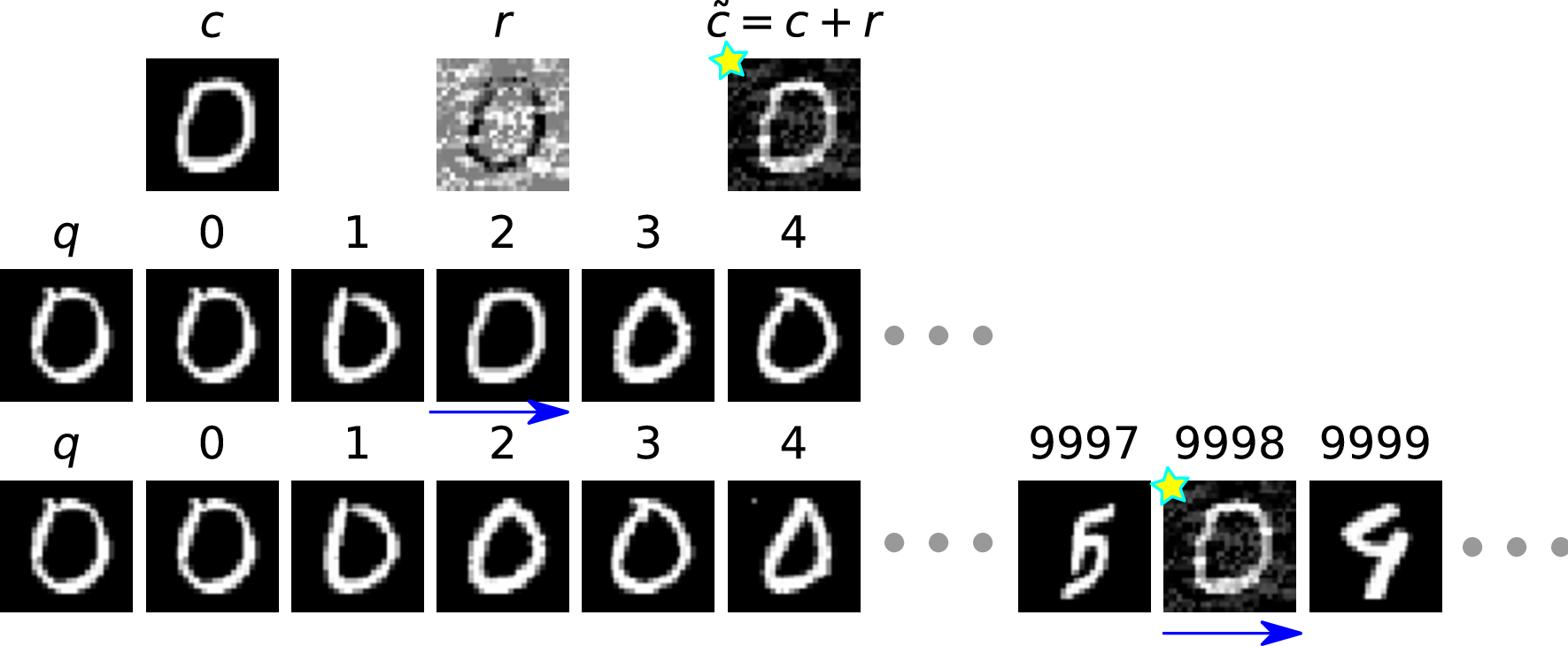
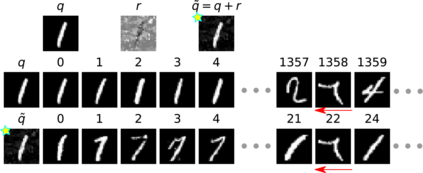
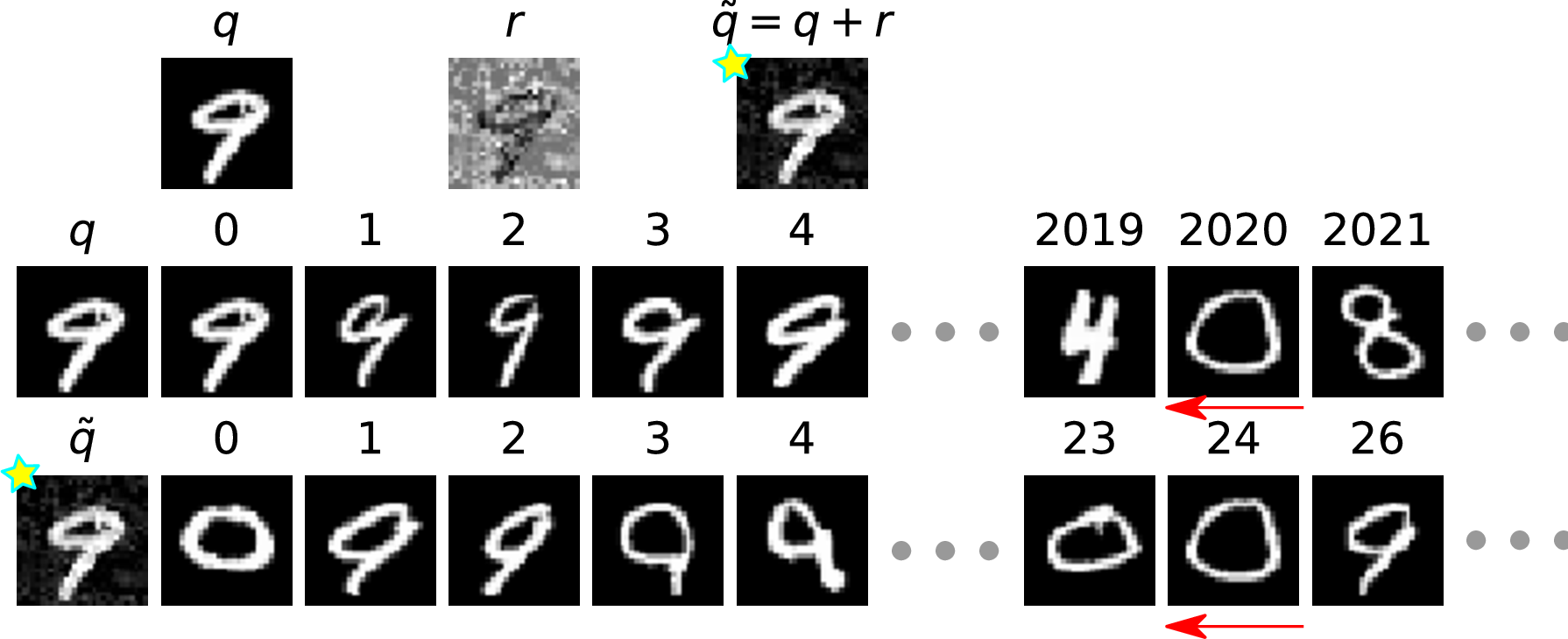
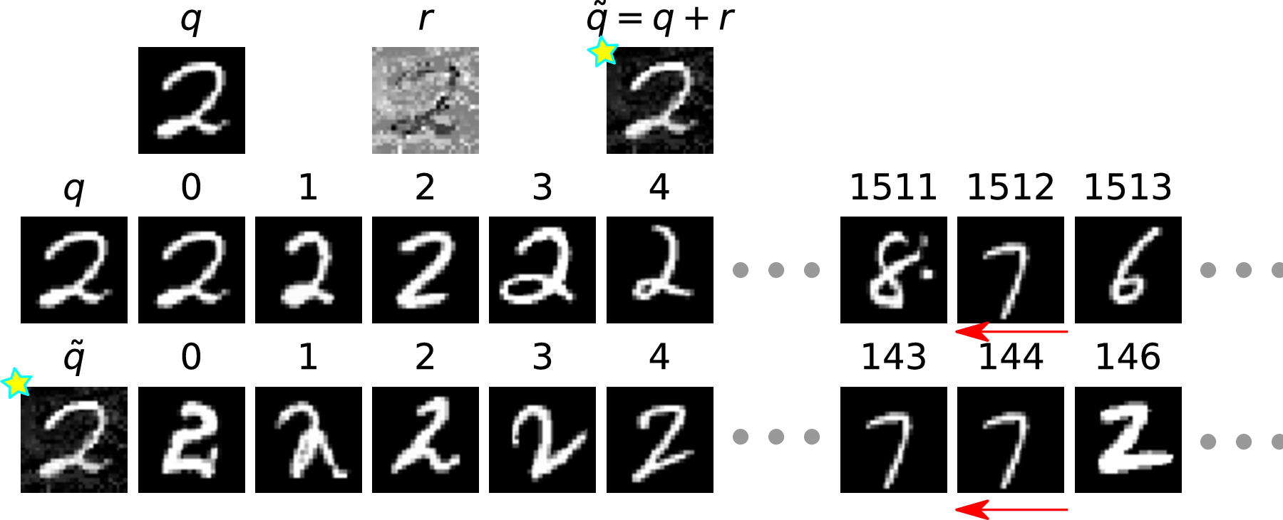
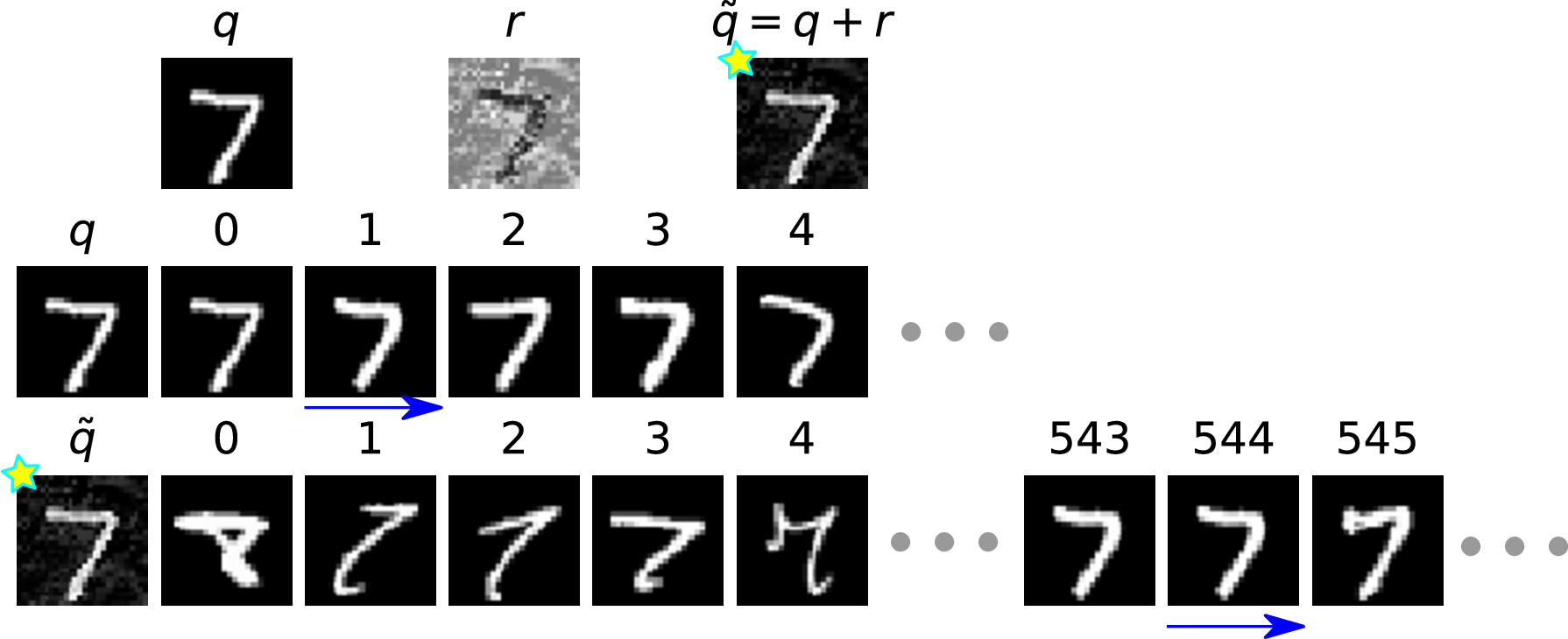
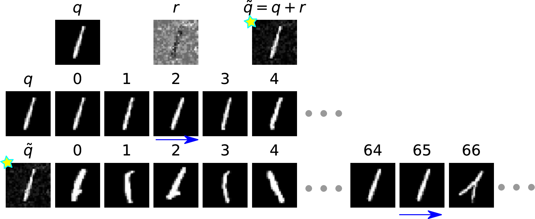
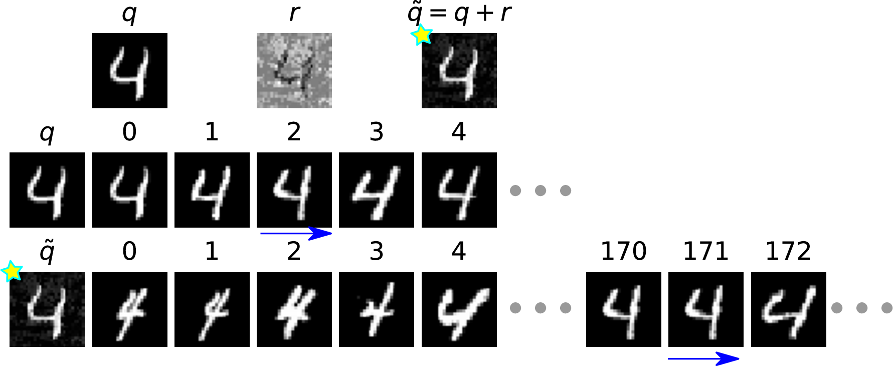
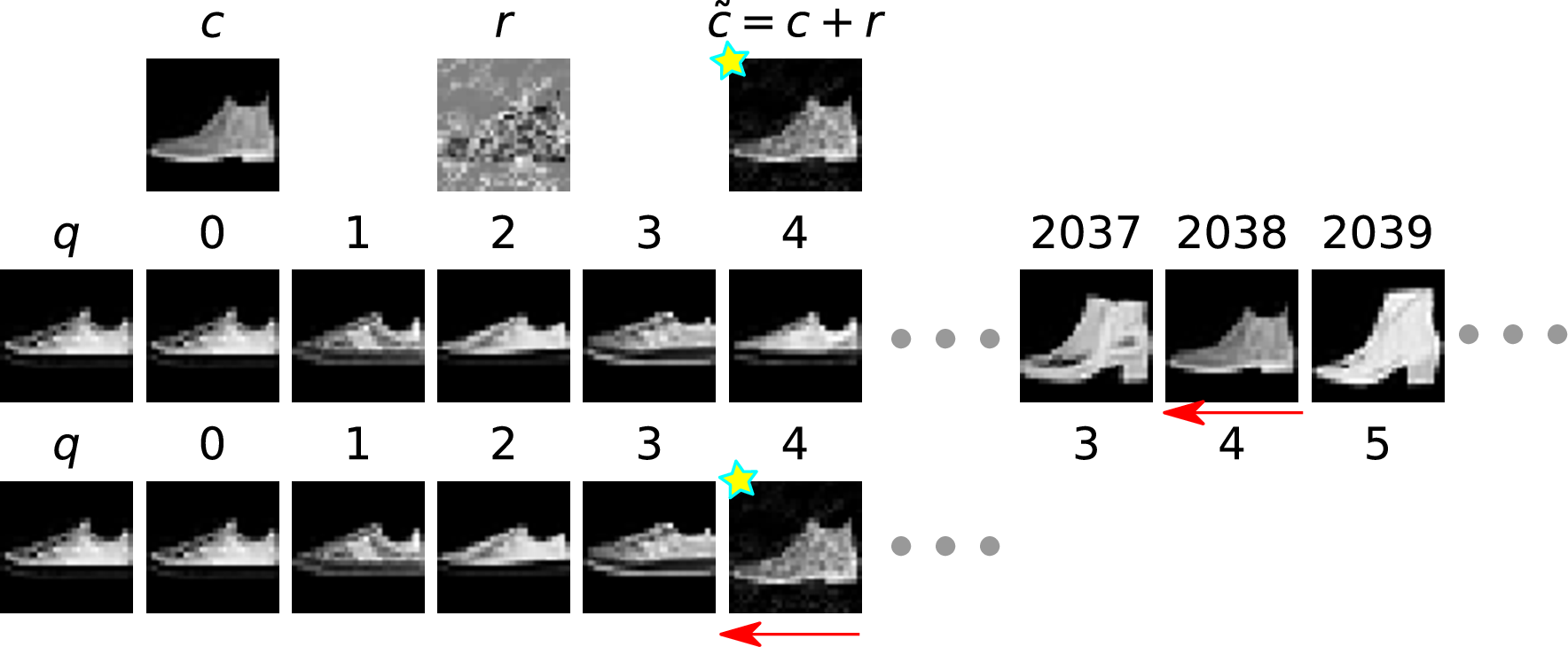
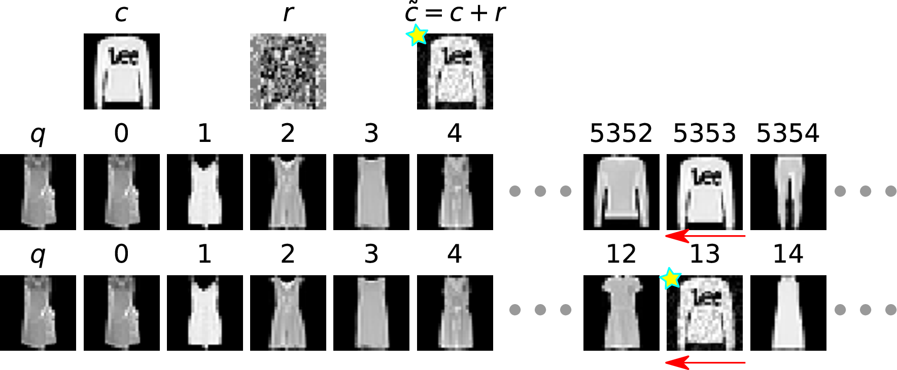
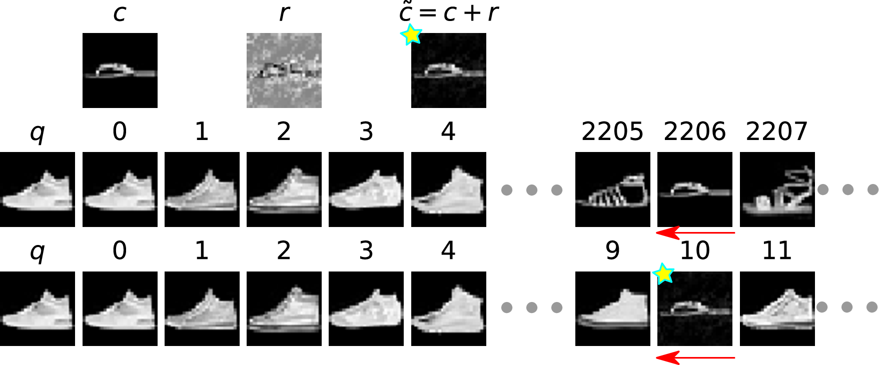
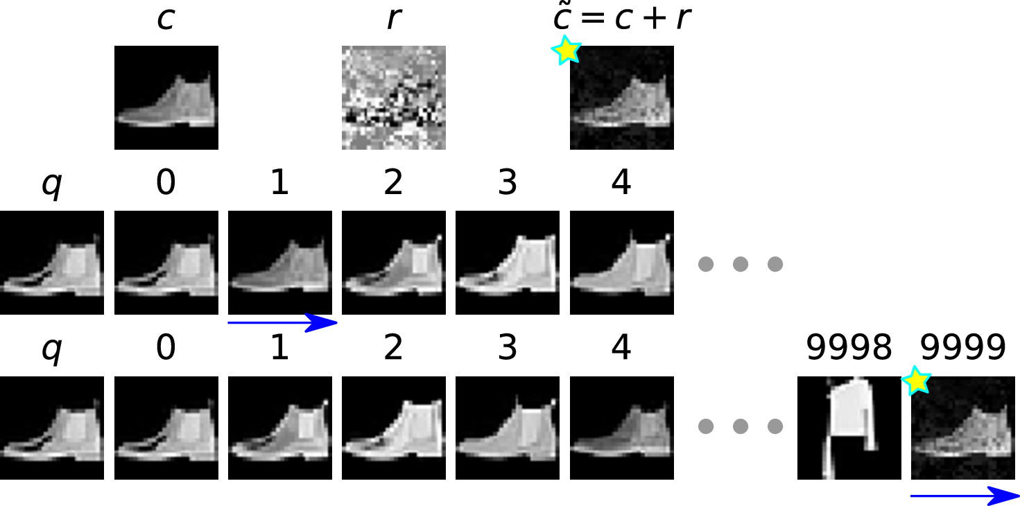
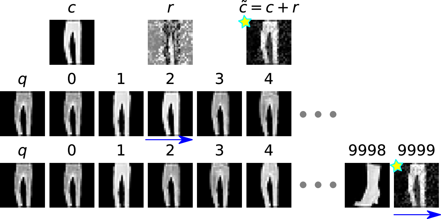
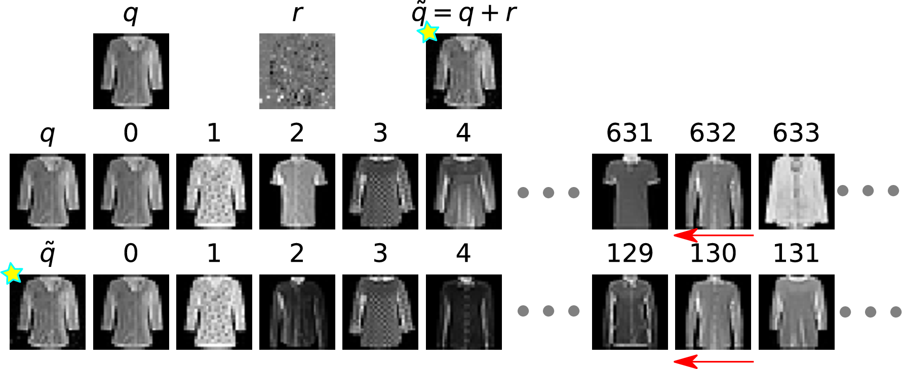
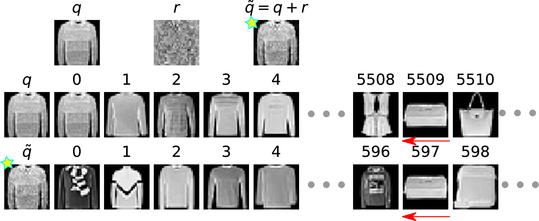
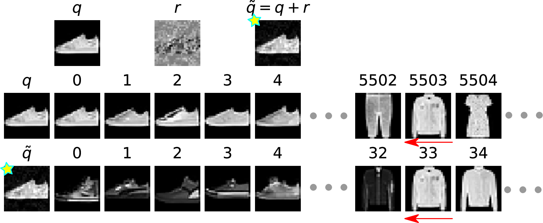
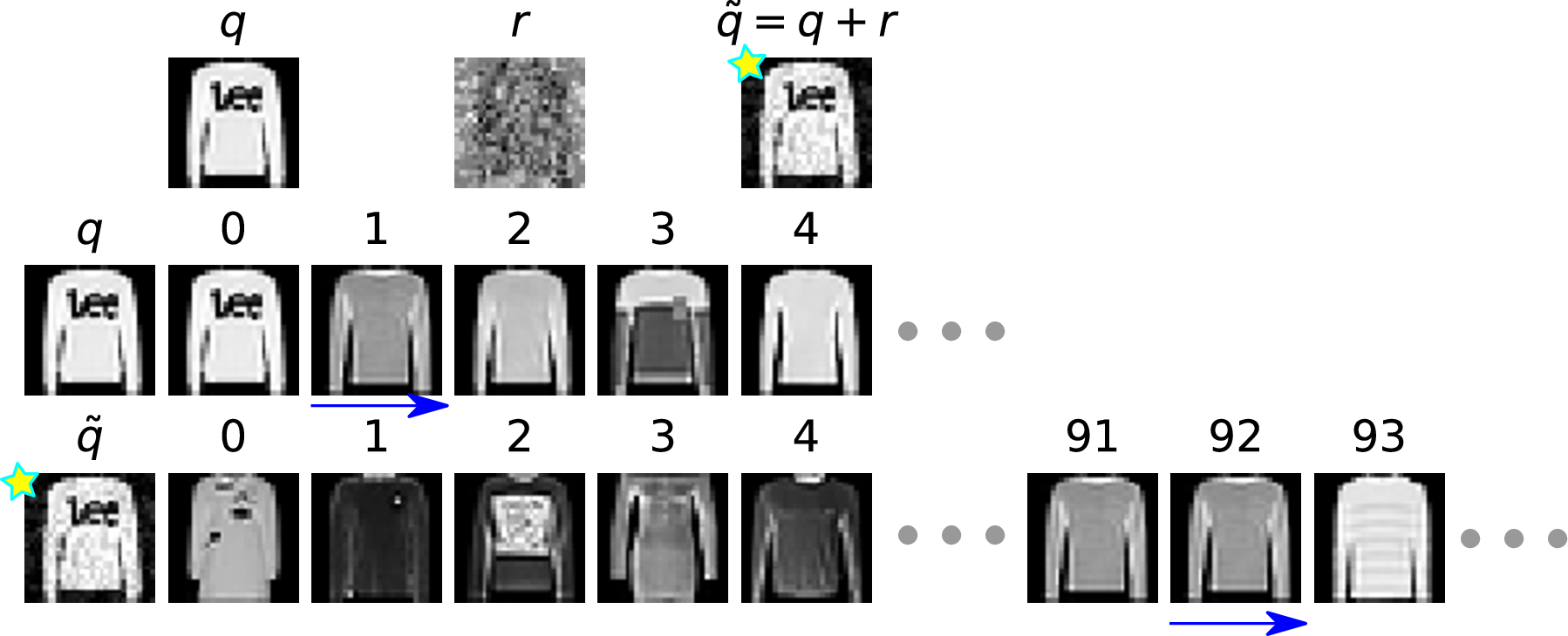
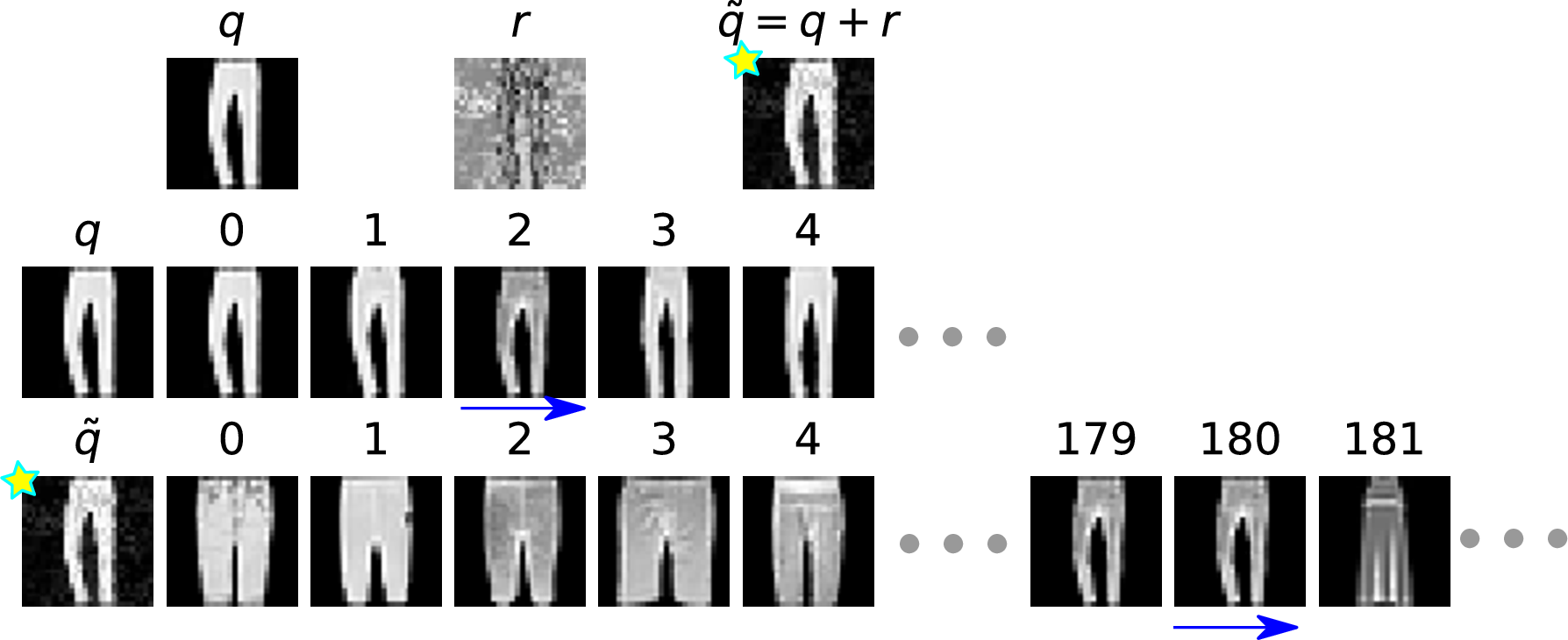
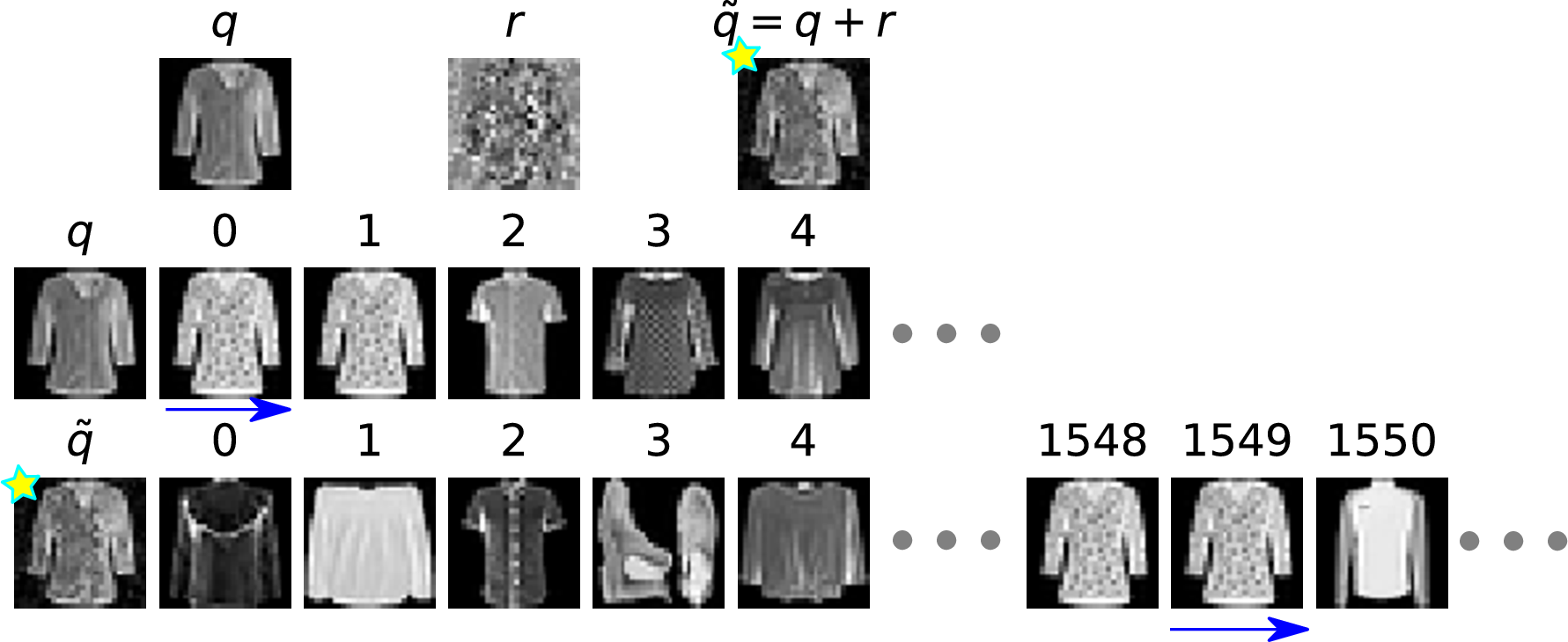
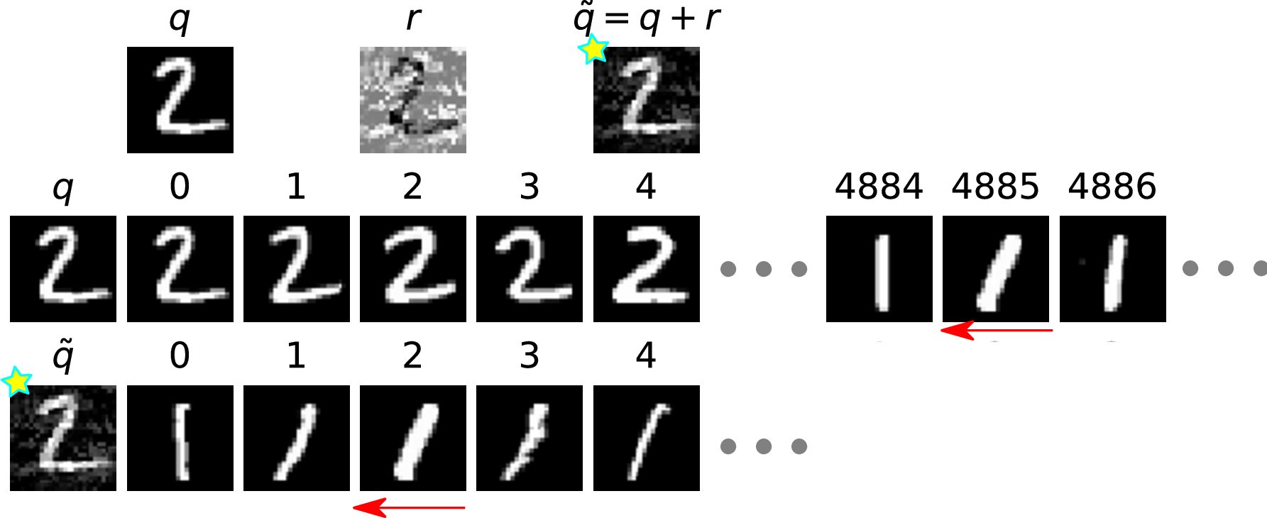
Some adversarial ranking examples are presented in this section. Every figure contains three rows of pictures. The first row shows \(c\), \(r\), \(\tilde{c}=c+r\) for CA, or \(q\), \(r\), \(\tilde{q}=q+r\) for QA. The second row shows the query and the original retrieval results, as well as the chosen candidate \(c\) and its immediately adjacent candidates. The third row shows the effects of the attack on the ranking list, , either the chosen candidate \(c\) is replaced with \(\tilde{c}\) for CA, or the query \(q\) is replaced with \(\tilde{q}\) for QA. The digits above every picture is the value of \(\text{Rank}_X(q,\cdot)-1\) 4.
Pictures with a ” ” mark on the top-left corner are adversarial examples. The “\(\leftarrow\)” indicates the chosen candidate whose rank will be raised. The “\(\rightarrow\)” indicates the chosen candidate whose rank will be lowered.
Full visualization results including those on SOP (removed from the Arxiv version due to file size limit) can be found at https://github.com/cdluminate/advrank-pub.
7.1 MNIST Dataset↩︎
CA+. See Fig. 3,4,5. CA-. See Fig. 6,7,8.
QA+. See Fig. 9,10,11. QA-. See Fig. 12,13,14.
7.2 Fashion-MNIST↩︎
CA+. See Fig. 15,16,17. CA-. See Fig. 18,19,20.
QA+. See Fig. 21,22,23. QA-. See Fig. 24,25,26.

7.3 Semantic-Preserving for QA↩︎
Conducting Query Attack without preserving the query semantics will often lead to irrelevant retrieval results at the top of the ranking list, as shown in Fig. 27, which raises red flags and possibly reveals the attack. Therefore, the value of the Semantics-Preserving term in QA is substantial, as it keeps the retrieval results as “normal” as possible while achieving the attacking goal.
8 Complete Results of Attack & Defense↩︎
Some experiments and details on MNIST, Fashion-MNIST and SOP datasets are omitted in the manuscript due to limited space. In this section, we present the complete experimental results on these datasets, including the average rank of \(C_\text{SP}\) during QA. Besides, we also conduct attacking experiments on ranking models trained with different combinations of loss functions and distance metrics. For brevity, we denote the (Cosine distance, Triplet loss) setting as (CT), the (Euclidean distance, Contrastive loss) as (EC). Models trained with our defense method will have a trailing “D” in notation, the (CT) model with our defense will be denoted as (CTD).
See Tab. 8 for complete results on MNIST.
See Tab. 9 for complete results on Fashion-MNIST.
See Tab. 7 for results on SOP.
| \(\varepsilon\) | CA+ | CA- | SP-QA+ | SP-QA- | ||||||||||||
| \(w=1\) | \(2\) | \(5\) | \(10\) | \(w=1\) | \(2\) | \(5\) | \(10\) | \(m=1\) | \(2\) | \(5\) | \(10\) | \(m=1\) | \(2\) | \(5\) | \(10\) | |
| 0 | 50 | 50 | 50 | 50 | 1.9 | 1.9 | 1.9 | 1.9 | 50 | 50 | 50 | 50 | 0.5 | 0.5 | 0.5 | 0.5 |
| 0.01 | 0.0 | 0.8 | 2.0 | 2.6 | 99.7 | 99.6 | 99.4 | 99.3 | 4.8, 0.2 | 7.0, 0.7 | 16.3, 1.9 | 25.8, 2.3 | 54.9, 0.3 | 40.2, 0.6 | 27.1, 0.8 | 21.9, 0.9 |
| 0.03 | 0.0 | 0.3 | 1.0 | 1.5 | 100.0 | 100.0 | 100.0 | 100.0 | 1.6, 0.1 | 3.3, 0.5 | 10.0, 2.0 | 19.2, 2.7 | 68.1, 0.3 | 52.4, 0.6 | 36.6, 0.8 | 30.1, 1.0 |
| 0.06 | 0.0 | 0.2 | 1.0 | 1.5 | 100.0 | 100.0 | 100.0 | 100.0 | 1.1, 0.2 | 2.7, 0.6 | 8.8, 1.9 | 17.6, 3.3 | 73.8, 0.4 | 57.9, 0.7 | 40.3, 0.8 | 32.4, 1.0 |
| 0 | 50 | 50 | 50 | 50 | 2.0 | 2.0 | 2.0 | 2.0 | 50 | 50 | 50 | 50 | 0.5 | 0.5 | 0.5 | 0.5 |
| 0.01 | 7.5 | 12.2 | 16.5 | 18.0 | 66.4 | 62.6 | 59.3 | 57.8 | 16.1, 2.1 | 24.8, 2.7 | 36.1, 2.7 | 41.4, 2.5 | 26.7, 0.6 | 18.1, 0.7 | 12.2, 0.7 | 10.2, 0.7 |
| 0.03 | 0.7 | 4.5 | 8.7 | 10.4 | 91.7 | 90.2 | 89.1 | 88.4 | 7.9, 2.9 | 14.5, 4.2 | 27.2, 5.4 | 35.6, 5.3 | 43.4, 1.3 | 31.7, 1.5 | 21.9, 1.7 | 18.1, 1.8 |
| 0.06 | 0.1 | 3.8 | 7.9 | 9.7 | 97.3 | 96.8 | 96.4 | 96.2 | 6.9, 4.3 | 12.5, 5.8 | 24.3, 7.0 | 33.4, 6.9 | 51.4, 2.8 | 39.0, 3.2 | 28.0, 3.5 | 23.5, 3.6 |
0.2em
| \(\varepsilon\) | CA+ | CA- | SP-QA+ | SP-QA- | ||||||||||||
| \(w=1\) | \(2\) | \(5\) | \(10\) | \(w=1\) | \(2\) | \(5\) | \(10\) | \(m=1\) | \(2\) | \(5\) | \(10\) | \(m=1\) | \(2\) | \(5\) | \(10\) | |
| 0 | 50 | 50 | 50 | 50 | 2.2 | 2.2 | 2.2 | 2.2 | 50 | 50 | 50 | 50 | 0.5 | 0.5 | 0.5 | 0.5 |
| 0.01 | 42.2 | 43.3 | 44.6 | 44.7 | 5.6 | 5.3 | 5.2 | 5.1 | 45.0, 0.5 | 46.9, 0.5 | 48.4, 0.5 | 49.1, 0.5 | 1.2, 0.5 | 1.2, 0.5 | 1.1, 0.5 | 1.1, 0.5 |
| 0.03 | 31.3 | 33.5 | 35.4 | 36.1 | 9.3 | 9.2 | 9.1 | 9.1 | 37.6, 2.3 | 41.7, 2.5 | 45.9, 2.5 | 47.7, 2.5 | 2.8, 1.8 | 2.7, 1.8 | 2.7, 1.8 | 2.6, 1.8 |
| 0.1 | 9.7 | 12.5 | 14.6 | 15.6 | 52.1 | 52.2 | 52.4 | 52.5 | 18.5, 8.2 | 27.1, 9.7 | 38.0, 9.9 | 43.4, 9.9 | 5.6, 4.1 | 5.4, 4.1 | 5.4, 4.1 | 5.4, 4.1 |
| 0.3 | 5.8 | 10.0 | 11.9 | 12.9 | 99.0 | 99.1 | 99.0 | 99.1 | 14.3, 9.7 | 23.3, 12.5 | 36.3, 13.8 | 42.6, 13.9 | 6.1, 4.4 | 5.8, 4.4 | 5.7, 4.4 | 5.7, 4.4 |
| 0 | 50 | 50 | 50 | 50 | 2.1 | 2.1 | 2.1 | 2.1 | 50 | 50 | 50 | 50 | 0.5 | 0.5 | 0.5 | 0.5 |
| 0.01 | 44.6 | 45.4 | 47.4 | 47.9 | 3.4 | 3.2 | 3.1 | 3.1 | 45.2, 0.0 | 46.3, 0.0 | 47.7, 0.0 | 48.5, 0.0 | 0.9, 0.0 | 0.7, 0.0 | 0.6, 0.0 | 0.6, 0.1 |
| 0.03 | 33.4 | 37.3 | 41.9 | 43.9 | 6.3 | 5.9 | 5.7 | 5.6 | 35.6, 0.3 | 39.2, 0.3 | 43.4, 0.3 | 45.8, 0.3 | 1.9, 0.2 | 1.4, 0.2 | 1.1, 0.2 | 1.1, 0.2 |
| 0.1 | 12.7 | 17.4 | 24.4 | 30.0 | 15.4 | 14.9 | 14.8 | 14.7 | 14.4, 2.2 | 21.0, 2.3 | 30.6, 2.3 | 37.2, 2.3 | 5.6, 1.2 | 4.4, 1.2 | 3.7, 1.2 | 3.5, 1.2 |
| 0.3 | 2.1 | 9.1 | 13.0 | 17.9 | 93.9 | 93.2 | 93.0 | 92.9 | 6.3, 3.6 | 11.2, 5.7 | 22.5, 7.7 | 32.1, 7.7 | 8.6, 1.6 | 6.6, 1.6 | 5.3, 1.5 | 4.8, 1.5 |
| 0 | 50 | 50 | 50 | 50 | 1.8 | 1.8 | 1.8 | 1.8 | 50 | 50 | 50 | 50 | 0.5 | 0.5 | 0.5 | 0.5 |
| 0.01 | 31.9 | 33.5 | 34.6 | 34.9 | 8.2 | 8.0 | 7.9 | 7.8 | 41.3, 2.0 | 44.0, 2.2 | 47.2, 2.4 | 48.4, 2.5 | 2.6, 1.3 | 2.4, 1.3 | 2.2, 1.3 | 2.2, 1.3 |
| 0.03 | 15.8 | 17.4 | 18.7 | 19.1 | 10.7 | 10.6 | 10.5 | 10.5 | 27.2, 4.8 | 34.6, 5.4 | 42.0, 5.6 | 45.6, 5.8 | 4.1, 2.5 | 3.9, 2.5 | 3.7, 2.5 | 3.7, 2.5 |
| 0.1 | 6.7 | 10.0 | 12.1 | 12.7 | 82.1 | 81.6 | 81.7 | 82.0 | 15.7, 9.8 | 25.4, 12.0 | 37.7, 13.1 | 43.2, 13.1 | 5.6, 3.2 | 5.3, 3.2 | 4.9, 3.2 | 4.9, 3.2 |
| 0.3 | 4.8 | 9.9 | 12.1 | 12.7 | 99.8 | 99.8 | 99.8 | 99.8 | 14.4, 9.4 | 23.9, 12.5 | 36.7, 13.6 | 42.6, 13.8 | 5.9, 3.2 | 5.4, 3.2 | 5.0, 3.2 | 4.9, 3.1 |
| 0 | 50 | 50 | 50 | 50 | 1.6 | 1.6 | 1.6 | 1.6 | 50 | 50 | 50 | 50 | 0.5 | 0.5 | 0.5 | 0.5 |
| 0.01 | 39.0 | 40.4 | 40.6 | 40.8 | 3.2 | 3.0 | 2.8 | 2.8 | 45.5, 0.1 | 47.4, 0.1 | 48.1, 0.1 | 49.0, 0.1 | 1.0, 0.1 | 0.9, 0.1 | 0.8, 0.1 | 0.8, 0.1 |
| 0.03 | 23.5 | 25.6 | 26.5 | 27.0 | 7.0 | 6.6 | 6.3 | 6.2 | 36.4, 0.6 | 40.9, 0.7 | 45.1, 0.8 | 47.1, 0.9 | 2.7, 0.7 | 2.3, 0.7 | 2.0, 0.7 | 2.0, 0.8 |
| 0.1 | 8.1 | 10.6 | 12.1 | 12.7 | 13.7 | 13.3 | 13.0 | 12.9 | 14.1, 4.8 | 23.4, 5.7 | 34.6, 6.2 | 40.8, 6.5 | 6.2, 1.7 | 5.1, 1.7 | 4.4, 1.7 | 4.2, 1.7 |
| 0.3 | 1.8 | 8.5 | 10.9 | 11.7 | 77.4 | 75.7 | 75.0 | 74.7 | 7.5, 5.2 | 15.0, 7.4 | 28.1, 9.0 | 36.3, 8.9 | 7.4, 1.7 | 5.8, 1.7 | 4.9, 1.7 | 4.6, 1.7 |
| 0 | 50 | 50 | 50 | 50 | 2.2 | 2.2 | 2.2 | 2.2 | 50 | 50 | 50 | 50 | 0.5 | 0.5 | 0.5 | 0.5 |
| 0.01 | 49.3 | 49.0 | 49.3 | 49.3 | 2.4 | 2.4 | 2.3 | 2.3 | 49.7, 0.0 | 49.6, 0.0 | 49.8, 0.0 | 49.9, 0.0 | 0.5, 0.0 | 0.5, 0.0 | 0.5, 0.0 | 0.5, 0.0 |
| 0.03 | 47.0 | 47.9 | 48.1 | 48.0 | 2.8 | 2.7 | 2.7 | 2.7 | 48.3, 0.0 | 49.1, 0.0 | 49.1, 0.0 | 49.4, 0.0 | 0.6, 0.0 | 0.5, 0.0 | 0.5, 0.0 | 0.5, 0.0 |
| 0.1 | 42.3 | 43.3 | 44.0 | 44.4 | 4.2 | 4.0 | 3.9 | 3.8 | 44.9 ,0.1 | 46.7 ,0.1 | 48.1 ,0.1 | 48.8 ,0.1 | 0.8 ,0.1 | 0.7 ,0.1 | 0.7 ,0.1 | 0.7 ,0.1 |
| 0.3 | 32.0 | 34.2 | 36.1 | 36.7 | 7.0 | 7.0 | 6.5 | 6.4 | 37.4, 0.6 | 41.1, 0.6 | 44.9, 0.5 | 47.2, 0.5 | 1.9, 0.5 | 1.6, 0.5 | 1.5, 0.5 | 1.5, 0.5 |
| 0 | 50 | 50 | 50 | 50 | 2.0 | 2.0 | 2.0 | 2.0 | 50 | 50 | 50 | 50 | 0.5 | 0.5 | 0.5 | 0.5 |
| 0.01 | 48.9 | 49.3 | 49.4 | 49.5 | 2.2 | 2.2 | 2.2 | 2.1 | 49.9, 0.0 | 49.5, 0.0 | 49.5, 0.0 | 49.7, 0.0 | 0.5, 0.0 | 0.5, 0.0 | 0.5, 0.0 | 0.5, 0.0 |
| 0.03 | 47.4 | 48.4 | 48.6 | 48.9 | 2.5 | 2.5 | 2.4 | 2.4 | 48.0, 0.0 | 48.5, 0.0 | 49.2, 0.0 | 49.5, 0.0 | 0.6, 0.0 | 0.6, 0.0 | 0.5, 0.0 | 0.5, 0.0 |
| 0.1 | 42.4 | 44.2 | 45.9 | 46.7 | 3.8 | 3.6 | 3.5 | 3.4 | 43.2, 0.1 | 45.0, 0.1 | 47.4, 0.1 | 48.2, 0.1 | 1.0, 0.1 | 0.8, 0.1 | 0.7, 0.1 | 0.7, 0.1 |
| 0.3 | 30.7 | 34.5 | 38.7 | 40.7 | 7.0 | 6.7 | 6.5 | 6.5 | 33.2, 0.5 | 37.2, 0.5 | 42.3, 0.5 | 45.1, 0.5 | 2.4, 0.4 | 1.9, 0.4 | 1.6, 0.4 | 1.5, 0.4 |
| 0 | 50 | 50 | 50 | 50 | 1.3 | 1.3 | 1.3 | 1.3 | 50 | 50 | 50 | 50 | 0.5 | 0.5 | 0.5 | 0.5 |
| 0.01 | 47.4 | 47.6 | 48.0 | 47.8 | 2.3 | 2.2 | 2.1 | 2.1 | 48.7, 0.1 | 49.1, 0.1 | 49.4, 0.1 | 49.7, 0.1 | 0.9, 0.1 | 0.8, 0.1 | 0.7, 0.1 | 0.7, 0.1 |
| 0.03 | 42.7 | 43.6 | 44.0 | 44.2 | 4.5 | 4.2 | 4.0 | 4.0 | 46.3, 0.6 | 48.1, 0.6 | 48.8, 0.6 | 49.2, 0.6 | 1.8, 0.6 | 1.6, 0.6 | 1.5, 0.6 | 1.4, 0.6 |
| 0.1 | 31.7 | 33.7 | 34.9 | 35.3 | 10.0 | 9.6 | 9.4 | 9.3 | 39.2, 2.8 | 43.2, 2.9 | 46.6, 2.9 | 47.9, 2.9 | 3.3, 1.3 | 2.9, 1.3 | 2.7, 1.3 | 2.6, 1.3 |
| 0.3 | 19.6 | 23.0 | 25.4 | 26.3 | 35.6 | 35.2 | 35.7 | 36.0 | 27.3, 7.1 | 34.4, 7.4 | 42.2, 7.1 | 45.4, 6.9 | 4.5, 1.8 | 3.9, 1.8 | 3.6, 1.8 | 3.4, 1.8 |
| 0 | 50 | 50 | 50 | 50 | 1.4 | 1.4 | 1.4 | 1.4 | 50 | 50 | 50 | 50 | 0.5 | 0.5 | 0.5 | 0.5 |
| 0.01 | 47.5 | 48.2 | 48.1 | 48.2 | 1.7 | 1.7 | 1.6 | 1.6 | 48.5, 0.0 | 48.8, 0.0 | 49.4, 0.0 | 49.7, 0.0 | 0.6, 0.0 | 0.6, 0.0 | 0.5, 0.0 | 0.5, 0.0 |
| 0.03 | 43.4 | 43.8 | 44.1 | 44.5 | 2.4 | 2.3 | 2.2 | 2.2 | 46.6, 0.0 | 47.8, 0.0 | 48.9, 0.1 | 49.3, 0.1 | 0.8, 0.1 | 0.7, 0.1 | 0.6, 0.1 | 0.6, 0.1 |
| 0.1 | 29.8 | 31.3 | 32.6 | 33.0 | 5.7 | 5.2 | 5.0 | 4.9 | 39.6, 0.3 | 42.9, 0.3 | 45.9, 0.4 | 47.9, 0.4 | 2.1, 0.4 | 1.7, 0.4 | 1.5, 0.4 | 1.4, 0.4 |
| 0.3 | 10.8 | 13.2 | 15.0 | 15.6 | 14.4 | 13.9 | 13.5 | 13.4 | 19.7, 3.2 | 28.1, 3.7 | 37.4, 4.1 | 42.6, 4.3 | 6.5, 1.7 | 5.3, 1.7 | 4.7, 1.8 | 4.5 1.8 |
| \(\varepsilon\) | CA+ | CA- | SP-QA+ | SP-QA- | ||||||||||||
| \(w=1\) | \(2\) | \(5\) | \(10\) | \(w=1\) | \(2\) | \(5\) | \(10\) | \(m=1\) | \(2\) | \(5\) | \(10\) | \(m=1\) | \(2\) | \(5\) | \(10\) | |
| 0 | 50 | 50 | 50 | 50 | 2.0 | 2.0 | 2.0 | 2.0 | 50 | 50 | 50 | 50 | 0.5 | 0.5 | 0.5 | 0.5 |
| 0.01 | 29.8 | 32.8 | 34.2 | 34.7 | 9.8 | 9.3 | 9.0 | 8.8 | 36.1, 1.6 | 40.3, 1.6 | 44.8, 1.5 | 46.9, 1.5 | 3.1, 1.4 | 2.8, 1.4 | 2.5, 1.4 | 2.5, 1.4 |
| 0.03 | 12.5 | 16.4 | 19.1 | 20.3 | 46.0 | 45.2 | 44.7 | 44.5 | 18.5, 4.6 | 25.7, 5.6 | 35.6, 5.9 | 41.6, 5.9 | 4.9, 2.4 | 4.4, 2.4 | 4.0, 2.4 | 3.9, 2.5 |
| 0.1 | 4.8 | 10.1 | 13.4 | 14.9 | 96.0 | 96.0 | 96.0 | 96.0 | 10.3, 7.0 | 17.3, 9.7 | 30.0, 11.1 | 38.2, 11.7 | 7.1, 3.7 | 6.4, 3.7 | 5.9, 3.7 | 5.7, 3.7 |
| 0.3 | 3.7 | 9.6 | 12.8 | 14.2 | 100.0 | 100.0 | 100.0 | 100.0 | 9.0, 6.3 | 15.7, 9.3 | 28.5, 11.3 | 37.5, 11.6 | 7.2, 3.5 | 6.4, 3.5 | 5.8, 3.5 | 5.6, 3.4 |
| 0 | 50 | 50 | 50 | 50 | 1.9 | 1.9 | 1.9 | 1.9 | 50 | 50 | 50 | 50 | 0.5 | 0.5 | 0.5 | 0.5 |
| 0.01 | 36.6 | 39.9 | 43.2 | 44.8 | 5.6 | 5.1 | 4.9 | 4.8 | 39.4, 0.2 | 42.0, 0.2 | 45.3, 0.2 | 47.1, 0.2 | 2.1, 0.2 | 1.6, 0.2 | 1.2, 0.2 | 1.1, 0.2 |
| 0.03 | 19.7 | 25.4 | 31.7 | 35.6 | 15.5 | 14.8 | 14.4 | 14.3 | 21.7, 1.5 | 28.2, 1.6 | 35.7, 1.7 | 40.6, 1.7 | 5.6, 0.8 | 4.1, 0.8 | 3.3, 0.8 | 2.9, 0.7 |
| 0.1 | 3.7 | 10.5 | 17.3 | 22.7 | 87.2 | 86.7 | 86.3 | 86.3 | 7.1, 2.4 | 12.4, 4.5 | 23.6, 6.9 | 32.5, 6.8 | 10.9, 1.9 | 8.3, 1.9 | 6.7, 1.9 | 6.0, 1.8 |
| 0.3 | 1.3 | 9.4 | 16.0 | 21.5 | 100.0 | 100.0 | 100.0 | 100.0 | 6.3, 3.0 | 10.8, 5.2 | 21.8, 7.8 | 31.7, 8.3 | 12.6, 1.9 | 9.4, 1.9 | 7.5, 1.9 | 6.6, 1.8 |
| 0 | 50 | 50 | 50 | 50 | 1.3 | 1.3 | 1.3 | 1.3 | 50 | 50 | 50 | 50 | 0.5 | 0.5 | 0.5 | 0.5 |
| 0.01 | 20.9 | 23.6 | 25.7 | 26.4 | 12.3 | 11.7 | 11.3 | 11.1 | 30.6, 3.7 | 36.7, 3.8 | 42.8, 3.9 | 45.8, 3.8 | 3.8, 1.6 | 3.3, 1.6 | 3.0, 1.6 | 2.9, 1.6 |
| 0.03 | 7.0 | 11.5 | 14.8 | 16.0 | 74.1 | 72.9 | 71.8 | 71.4 | 15.7, 8.0 | 25.4, 9.3 | 36.9, 9.1 | 42.4, 8.8 | 4.6, 2.0 | 4.0, 2.0 | 3.6, 2.0 | 3.6, 2.1 |
| 0.1 | 6.2 | 12.2 | 17.0 | 18.7 | 100.0 | 100.0 | 100.0 | 100.0 | 14.2, 9.3 | 22.6, 12.3 | 34.8, 13.2 | 41.2, 13.0 | 8.3, 4.7 | 7.8, 4.8 | 7.3, 4.8 | 7.1, 4.8 |
| 0.3 | 5.7 | 12.0 | 16.5 | 18.2 | 100.0 | 100.0 | 100.0 | 100.0 | 12.8, 9.0 | 21.1, 11.9 | 33.8, 13.5 | 40.4, 13.4 | 9.1, 5.1 | 8.4, 5.2 | 7.9, 5.0 | 7.5, 4.9 |
| 0 | 50 | 50 | 50 | 50 | 1.5 | 1.5 | 1.5 | 1.5 | 50 | 50 | 50 | 50 | 0.5 | 0.5 | 0.5 | 0.5 |
| 0.01 | 33.2 | 34.8 | 34.7 | 36.1 | 6.5 | 5.9 | 5.5 | 5.3 | 41.7, 0.3 | 44.4, 0.3 | 47.3, 0.3 | 48.4, 0.3 | 2.5, 0.3 | 1.9, 0.3 | 1.6, 0.3 | 1.4, 0.3 |
| 0.03 | 14.0 | 17.6 | 20.3 | 21.3 | 18.4 | 17.2 | 16.4 | 16.0 | 22.2, 2.5 | 30.0, 2.7 | 39.4, 2.7 | 43.6, 2.6 | 6.6, 1.3 | 5.1, 1.4 | 4.2, 1.4 | 3.9, 1.4 |
| 0.1 | 1.7 | 9.5 | 14.0 | 15.6 | 88.3 | 86.7 | 85.2 | 84.5 | 8.0, 3.9 | 15.0, 6.3 | 27.6, 7.9 | 36.5, 8.1 | 10.5, 1.9 | 8.0, 1.9 | 6.4, 2.0 | 6.0, 2.0 |
| 0.3 | 0.3 | 9.0 | 13.8 | 15.5 | 100.0 | 100.0 | 100.0 | 100.0 | 6.7, 3.3 | 12.6, 5.7 | 25.4, 7.9 | 34.8, 8.3 | 11.9, 1.9 | 8.9, 1.9 | 7.1, 1.9 | 6.4, 1.9 |
| 0 | 50 | 50 | 50 | 50 | 2.0 | 2.0 | 2.0 | 2.0 | 50 | 50 | 50 | 50 | 0.5 | 0.5 | 0.5 | 0.5 |
| 0.01 | 47.0 | 47.7 | 47.8 | 47.9 | 2.3 | 2.3 | 2.3 | 2.2 | 48.9, 0.0 | 48.7, 0.0 | 49.2, 0.0 | 49.6, 0.0 | 0.6, 0.0 | 0.5, 0.0 | 0.5, 0.0 | 0.5, 0.0 |
| 0.03 | 42.2 | 43.3 | 44.1 | 44.3 | 3.1 | 3.0 | 2.9 | 2.8 | 45.2, 0.0 | 47.2, 0.0 | 48.0, 0.0 | 49.1, 0.0 | 0.8, 0.0 | 0.7, 0.0 | 0.6, 0.0 | 0.6, 0.0 |
| 0.1 | 29.1 | 31.4 | 32.9 | 33.8 | 8.0 | 7.1 | 6.4 | 6.2 | 34.7, 0.1 | 39.5, 0.1 | 43.8, 0.1 | 46.5, 0.1 | 3.3, 0.1 | 2.1, 0.1 | 1.5, 0.1 | 1.3, 0.1 |
| 0.3 | 11.8 | 14.8 | 17.4 | 18.4 | 28.7 | 25.5 | 23.1 | 22.4 | 13.3, 0.7 | 20.0, 0.9 | 31.0, 1.0 | 38.3, 1.0 | 21.3, 1.0 | 14.3, 1.0 | 10.3, 1.0 | 8.6, 1.1 |
| 0 | 50 | 50 | 50 | 50 | 1.2 | 1.2 | 1.2 | 1.2 | 50 | 50 | 50 | 50 | 0.5 | 0.5 | 0.5 | 0.5 |
| 0.01 | 48.9 | 48.9 | 49.3 | 49.3 | 1.4 | 1.4 | 1.4 | 1.4 | 49.4, 0.0 | 49.9, 0.0 | 49.9, 0.0 | 50.0, 0.0 | 0.5, 0.0 | 0.5, 0.0 | 0.5, 0.0 | 0.5, 0.0 |
| 0.03 | 47.1 | 47.9 | 48.3 | 48.3 | 2.0 | 1.9 | 1.8 | 1.8 | 48.3, 0.0 | 49.1, 0.0 | 49.5, 0.0 | 49.8, 0.0 | 0.7, 0.0 | 0.6, 0.0 | 0.6, 0.0 | 0.6, 0.0 |
| 0.1 | 42.4 | 43.5 | 44.5 | 44.8 | 4.6 | 4.2 | 4.0 | 3.9 | 45.4, 0.3 | 47.2, 0.2 | 48.7, 0.2 | 49.2, 0.2 | 1.4, 0.2 | 1.2, 0.2 | 1.1, 0.2 | 1.0, 0.2 |
| 0.3 | 32.5 | 35.4 | 37.5 | 38.2 | 11.2 | 10.5 | 10.1 | 10.0 | 39.3, 1.5 | 42.6, 1.5 | 46.5, 1.3 | 47.8, 1.3 | 3.9, 1.4 | 3.3, 1.4 | 3.0, 1.4 | 2.9, 1.4 |
| 0 | 50 | 50 | 50 | 50 | 1.4 | 1.4 | 1.4 | 1.4 | 50 | 50 | 50 | 50 | 0.5 | 0.5 | 0.5 | 0.5 |
| 0.01 | 45.3 | 45.8 | 46.3 | 46.6 | 3.0 | 2.8 | 2.7 | 2.6 | 48.0, 0.2 | 48.7, 0.2 | 49.3, 0.3 | 49.7, 0.3 | 1.2, 0.2 | 1.0, 0.2 | 0.9, 0.2 | 0.9, 0.2 |
| 0.03 | 37.6 | 39.5 | 40.4 | 40.7 | 7.5 | 7.0 | 6.8 | 6.7 | 43.9, 1.5 | 46.4, 1.6 | 48.4, 1.7 | 49.1, 1.9 | 2.7, 0.7 | 2.2, 0.7 | 1.9, 0.7 | 1.9, 0.7 |
| 0.1 | 20.3 | 24.9 | 27.8 | 28.6 | 32.6 | 32.1 | 32.0 | 32.5 | 28.4, 6.6 | 36.2, 7.2 | 43.0, 7.4 | 45.9, 7.4 | 5.3, 1.5 | 4.4, 1.6 | 3.8, 1.6 | 3.7, 1.6 |
| 0.3 | 7.3 | 16.0 | 21.1 | 22.5 | 78.0 | 79.0 | 80.3 | 81.2 | 14.0, 10.2 | 24.6, 11.9 | 36.5, 11.8 | 42.2, 11.2 | 7.0, 1.9 | 5.7, 1.9 | 4.9, 1.9 | 4.6, 1.9 |
| 0 | 50 | 50 | 50 | 50 | 1.3 | 1.3 | 1.3 | 1.3 | 50 | 50 | 50 | 50 | 0.5 | 0.5 | 0.5 | 0.5 |
| 0.01 | 46.0 | 46.7 | 46.9 | 46.7 | 2.0 | 1.9 | 1.8 | 1.8 | 48.1, 0.0 | 49.1, 0.0 | 49.3, 0.0 | 49.6, 0.0 | 0.8, 0.0 | 0.7, 0.0 | 0.6, 0.0 | 0.6, 0.1 |
| 0.03 | 38.9 | 40.6 | 41.2 | 41.4 | 4.3 | 3.8 | 3.5 | 3.4 | 45.2, 0.2 | 46.2, 0.1 | 48.1, 0.1 | 48.9, 0.1 | 1.9, 0.2 | 1.5, 0.2 | 1.2, 0.2 | 1.1, 0.2 |
| 0.1 | 23.0 | 26.3 | 28.0 | 28.8 | 15.9 | 14.9 | 14.2 | 13.9 | 31.8, 1.8 | 38.0, 1.8 | 43.3, 1.6 | 46.2, 1.6 | 5.6, 1.0 | 4.3, 1.0 | 3.6, 1.0 | 3.3, 1.0 |
| 0.3 | 7.1 | 13.9 | 18.4 | 19.9 | 54.1 | 51.8 | 50.0 | 49.2 | 10.6, 5.6 | 19.7, 7.1 | 32.5, 8.0 | 39.6, 7.6 | 9.2, 1.6 | 7.0, 1.6 | 5.6, 1.6 | 5.1, 1.6 |
0.2em
9 Complete Results on Transferability↩︎
9.1 Fashion-MNIST↩︎
In addition to the transferability experiment on MNIST dataset, we also conduct the same transferability experiment on the Fashion-MNIST dataset, as shown in Tab. ¿tbl:tab:transfer-fashion?.
0.2em
| LeNet | C2F1 | Res18 | |
| LeNet | 50\(\rightarrow\)16.0 | 41.0 | 44.3 |
| C2F1 | 38.6 | 50\(\rightarrow\)1.3 | 40.3 |
| Res18 | 39.2 | 34.3 | 50\(\rightarrow\)1.7 |
| LeNet | C2F1 | Res18 | |
| LeNet | 2.5\(\rightarrow\)84.3 | 1.9\(\rightarrow\)8.1 | 1.6\(\rightarrow\)6.0 |
| C2F1 | 2.5\(\rightarrow\)7.8 | 1.9\(\rightarrow\)100.0 | 1.7\(\rightarrow\)7.7 |
| Res18 | 2.5\(\rightarrow\)9.5 | 1.9\(\rightarrow\)14.4 | 1.7\(\rightarrow\)80.0 |
| LeNet | C2F1 | Res18 | |
| LeNet | 50\(\rightarrow\)18.0 | 47.2 | 49.3 |
| C2F1 | 48.1 | 50\(\rightarrow\)6.4 | 49.2 |
| Res18 | 48.1 | 44.8 | 50\(\rightarrow\)13.7 |
| LeNet | C2F1 | Res18 | |
| LeNet | 0.5\(\rightarrow\)13.5 | 0.5\(\rightarrow\)1.7 | 0.5\(\rightarrow\)1.5 |
| C2F1 | 0.5\(\rightarrow\)1.1 | 0.5\(\rightarrow\)12.5 | 0.5\(\rightarrow\)1.6 |
| Res18 | 0.5\(\rightarrow\)0.9 | 0.5\(\rightarrow\)1.3 | 0.5\(\rightarrow\)8.0 |
9.2 “Self-Transfer” Attack on MNIST↩︎
| C2F1-1 | C2F1-2 | C2F1-3 | C2F1-D1 | C2F1-D2 | |
| C2F1-1 | 50\(\rightarrow\)2.1 | 27.9 | 25.3 | 45.3 | 45.1 |
| C2F1-2 | 24.4 | 50\(\rightarrow\)2.7 | 23.7 | 44.5 | 44.0 |
| C2F1-3 | 22.6 | 24.4 | 50\(\rightarrow\)2.2 | 45.0 | 44.5 |
| C2F1-D1 | 36.7 | 37.7 | 37.4 | 50\(\rightarrow\)30.9 | 38.6 |
| C2F1-D2 | 37.3 | 36.8 | 37.3 | 39.6 | 50\(\rightarrow\)30.3 |
| C2F1-1 | C2F1-2 | C2F1-3 | C2F1-D1 | C2F1-D2 | |
| C2F1-1 | 2.1\(\rightarrow\)93.7 | 2.2\(\rightarrow\)9.4 | 2.1\(\rightarrow\)11.1 | 2.0\(\rightarrow\)3.2 | 1.9\(\rightarrow\)3.1 |
| C2F1-2 | 2.1\(\rightarrow\)13.5 | 2.1\(\rightarrow\)88.1 | 2.2\(\rightarrow\)12.3 | 2.0\(\rightarrow\)3.4 | 1.9\(\rightarrow\)3.3 |
| C2F1-3 | 2.1\(\rightarrow\)13.4 | 2.2\(\rightarrow\)10.1 | 2.2\(\rightarrow\)92.4 | 2.0\(\rightarrow\)3.2 | 1.9\(\rightarrow\)3.2 |
| C2F1-D1 | 2.1\(\rightarrow\)9.3 | 2.2\(\rightarrow\)8.3 | 2.1\(\rightarrow\)9.1 | 2.0\(\rightarrow\)7.0 | 2.0\(\rightarrow\)4.9 |
| C2F1-D2 | 2.1\(\rightarrow\)9.2 | 2.2\(\rightarrow\)8.4 | 2.1\(\rightarrow\)9.1 | 2.0\(\rightarrow\)4.9 | 1.9\(\rightarrow\)7.0 |
| C2F1-1 | C2F1-2 | C2F1-3 | C2F1-D1 | C2F1-D2 | |
| C2F1-1 | 50\(\rightarrow\)6.4 | 39.4 | 38.1 | 48.6 | 48.1 |
| C2F1-2 | 36.6 | 50\(\rightarrow\)6.3 | 36.4 | 47.3 | 48.4 |
| C2F1-3 | 36.9 | 37.8 | 50\(\rightarrow\)6.2 | 48.7 | 48.3 |
| C2F1-D1 | 41.5 | 40.3 | 41.4 | 50\(\rightarrow\)32.9 | 40.6 |
| C2F1-D2 | 41.7 | 38.9 | 41.7 | 41.4 | 50\(\rightarrow\)32.7 |
| C2F1-1 | C2F1-2 | C2F1-3 | C2F1-D1 | C2F1-D2 | |
| C2F1-1 | 0.5\(\rightarrow\)8.8 | 0.5\(\rightarrow\)1.4 | 0.5\(\rightarrow\)1.9 | 0.5\(\rightarrow\)0.6 | 0.5\(\rightarrow\)0.6 |
| C2F1-2 | 0.5\(\rightarrow\)2.3 | 0.5\(\rightarrow\)9.0 | 0.5\(\rightarrow\)2.2 | 0.5\(\rightarrow\)0.6 | 0.5\(\rightarrow\)0.6 |
| C2F1-3 | 0.5\(\rightarrow\)1.9 | 0.5\(\rightarrow\)1.5 | 0.5\(\rightarrow\)8.7 | 0.5\(\rightarrow\)0.6 | 0.5\(\rightarrow\)0.6 |
| C2F1-D1 | 0.5\(\rightarrow\)5.8 | 0.5\(\rightarrow\)3.1 | 0.5\(\rightarrow\)4.8 | 0.5\(\rightarrow\)2.4 | 0.5\(\rightarrow\)1.3 |
| C2F1-D2 | 0.5\(\rightarrow\)7.1 | 0.5\(\rightarrow\)3.7 | 0.5\(\rightarrow\)5.9 | 0.5\(\rightarrow\)1.3 | 0.5\(\rightarrow\)2.4 |
0.2em
In the adversarial ranking example transferability experiments, we transfer adversarial examples between neural networks with different architectures. In this section, we transfer adversarial examples between neural networks based on the same architecture but with different parameters.
We train three vanilla C2F1 models (denoted as C2F1-1, C2F1-2, and C2f1-3) on MNIST dataset and two models with our defense (denoted as C2F1-D1, C2F1-D2). All these models have exactly the same architecture, but different parameters. Transferability experimental results between these models are present in Tab. 10.
10 Complete Results for Universal Perturbation↩︎
10.1 MNIST↩︎
See Tab. 5.
| Model | I-CA+ (\(w=1\)) | I-CA- (\(w=1\)) | I-QA+ (\(m=1\)) | I-QA- (\(m=1\)) | ||||
| Seen | Unseen | Seen | Unseen | Seen | Unseen | Seen | Unseen | |
| (CC) | 50 \(\rightarrow\) 13.7 | 50 \(\rightarrow\) 14.1 | 0.6 \(\rightarrow\) 37.6 | 0.6 \(\rightarrow\) 33.4 | 50 \(\rightarrow\) 18.1 | 50 \(\rightarrow\) 18.9 | 2.4 \(\rightarrow\) 41.6 | 2.4 \(\rightarrow\) 39.3 |
| (CT) | 50 \(\rightarrow\) 18.1 | 50 \(\rightarrow\) 18.5 | 0.6 \(\rightarrow\) 9.5 | 0.7 \(\rightarrow\) 9.4 | 50 \(\rightarrow\) 20.5 | 50 \(\rightarrow\) 21.0 | 2.1 \(\rightarrow\) 7.6 | 2.2 \(\rightarrow\) 7.4 |
| (EC) | 50 \(\rightarrow\) 9.1 | 50 \(\rightarrow\) 10.3 | 1.9 \(\rightarrow\) 94.6 | 2.0 \(\rightarrow\) 79.4 | 50 \(\rightarrow\) 3.9 | 50 \(\rightarrow\) 6.9 | 3.3 \(\rightarrow\) 87.1 | 3.5 \(\rightarrow\) 74.4 |
| (ET) | 50 \(\rightarrow\) 11.5 | 50 \(\rightarrow\) 12.6 | 2.1 \(\rightarrow\) 10.6 | 2.1 \(\rightarrow\) 9.6 | 50 \(\rightarrow\) 21.6 | 50 \(\rightarrow\) 23.6 | 3.2 \(\rightarrow\) 28.6 | 3.2 \(\rightarrow\) 19.5 |
0.2em
10.2 Fashion-MNIST↩︎
As shown in Tab. 12, Image-agnostic adversarial perturbation has better effect on seen data from Fashion-MNIST, but the gap between the effect on seen samples and that on unseen samples is slightly larger, which may due to the higher intra-class variance of Fashion-MNIST than MNIST.
| Model | I-CA+ (\(w=1\)) | I-CA- (\(w=1\)) | I-QA+ (\(m=1\)) | I-QA- (\(m=1\)) | ||||
| Seen | Unseen | Seen | Unseen | Seen | Unseen | Seen | Unseen | |
| (CC) | 50 \(\rightarrow\) 7.0 | 50 \(\rightarrow\) 7.3 | 0.6 \(\rightarrow\) 91.8 | 0.6 \(\rightarrow\) 84.9 | 50 \(\rightarrow\) 4.4 | 50 \(\rightarrow\) 4.9 | 2.1 \(\rightarrow\) 87.5 | 2.1 \(\rightarrow\) 84.4 |
| (CT) | 50 \(\rightarrow\) 9.8 | 50 \(\rightarrow\) 9.9 | 0.6 \(\rightarrow\) 72.3 | 0.6 \(\rightarrow\) 69.7 | 50 \(\rightarrow\) 8.2 | 50 \(\rightarrow\) 8.4 | 2.0 \(\rightarrow\) 76.3 | 2.0 \(\rightarrow\) 72.9 |
| (EC) | 50 \(\rightarrow\) 5.8 | 50 \(\rightarrow\) 9.6 | 2.0 \(\rightarrow\) 97.5 | 1.9 \(\rightarrow\) 83.7 | 50 \(\rightarrow\) 1.8 | 50 \(\rightarrow\) 7.1 | 2.9 \(\rightarrow\) 87.9 | 2.8 \(\rightarrow\) 78.4 |
| (ET) | 50 \(\rightarrow\) 5.7 | 50 \(\rightarrow\) 8.5 | 2.0 \(\rightarrow\) 84.4 | 1.9 \(\rightarrow\) 69.9 | 50 \(\rightarrow\) 3.3 | 50 \(\rightarrow\) 6.3 | 3.1 \(\rightarrow\) 88.0 | 3.0 \(\rightarrow\) 78.0 |
0.2em
11 Complete Parameter Search on \(\xi\)↩︎
See Tab. 13.
| \(\xi\) | SP-QA+ | SP-QA- | ||||||
| m=1 | 2 | 5 | 10 | m=1 | 2 | 5 | 10 | |
| 0 | 1.4, 43.9 | 13.8, 38.1 | 30.7, 37.9 | 39.4, 36.3 | 94.7, 93.3 | 94.4, 93.5 | 94.2, 93.7 | 94.1, 93.8 |
| \(10^0\) | 14.3, 9.7 | 23.3, 12.5 | 36.3, 13.8 | 42.6, 13.9 | 40.6, 37.6 | 40.6, 38.1 | 40.4, 38.1 | 39.8, 37.7 |
| \(10^2\) | 25.4, 2.0 | 33.2, 2.1 | 41.7, 2.1 | 45.4, 2.1 | 6.1, 4.4 | 5.8, 4.4 | 5.7, 4.4 | 5.7, 4.4 |
| \(10^4\) | 48.1, 0.3 | 49.2, 0.2 | 49.6, 0.2 | 49.8, 0.3 | 1.2, 0.3 | 1.1, 0.3 | 1.1, 0.3 | 1.1, 0.3 |
| 0 | 0.2, 33.6 | 6.3, 23.7 | 18.5, 26.5 | 29.6, 25.7 | 94.1, 89.4 | 93.2, 90.3 | 92.6, 90.9 | 92.3, 91.2 |
| \(10^0\) | 6.3, 3.6 | 11.2, 5.7 | 22.5, 7.7 | 32.1, 7.7 | 55.5, 35.6 | 52.4, 37.6 | 50.2, 39.3 | 49.4, 40.0 |
| \(10^2\) | 14.1, 0.6 | 20.8, 0.7 | 31.2, 0.7 | 38.1, 0.7 | 8.6, 1.6 | 6.6, 1.6 | 5.3, 1.5 | 4.8, 1.5 |
| \(10^4\) | 37.9, 0.1 | 42.6, 0.1 | 46.3, 0.1 | 47.8, 0.1 | 1.9, 0.1 | 1.4, 0.1 | 1.2, 0.1 | 1.1, 0.1 |
| 0 | 0.7, 44.5 | 13.4, 39.9 | 31.0, 41.8 | 39.7, 41.6 | 94.0, 92.6 | 93.9, 93.0 | 93.9, 93.4 | 93.9, 93.5 |
| \(10^0\) | 14.4, 9.4 | 23.9, 12.5 | 36.7, 13.6 | 42.6, 13.8 | 39.9, 37.6 | 39.0, 37.2 | 39.2, 37.7 | 38.7, 37.3 |
| \(10^2\) | 30.1, 1.2 | 37.3, 1.1 | 43.9, 0.9 | 46.7, 0.9 | 5.9, 3.2 | 5.4, 3.2 | 5.0, 3.2 | 4.9, 3.1 |
| \(10^4\) | 50.1, 0.8 | 50.2, 0.8 | 49.8, 0.8 | 50.0, 0.8 | 1.6, 0.7 | 1.6, 0.7 | 1.7, 0.8 | 1.6, 0.8 |
| 0 | 0.6, 37.4 | 8.2, 35.1 | 22.6, 38.2 | 33.2, 38.8 | 93.0, 88.4 | 92.5, 89.9 | 92.3, 90.9 | 92.1, 90.9 |
| \(10^0\) | 7.5, 5.2 | 15.0, 7.4 | 28.1, 9.0 | 36.3, 8.9 | 50.9, 37.3 | 49.2, 39.4 | 47.7, 40.6 | 47.2, 40.9 |
| \(10^2\) | 20.3, 0.5 | 28.6, 0.5 | 38.2, 0.5 | 43.1, 0.4 | 7.4, 1.7 | 5.8, 1.7 | 4.9, 1.7 | 4.6, 1.7 |
| \(10^4\) | 46.2, 0.1 | 48.2, 0.1 | 49.1, 0.1 | 49.6, 0.1 | 1.7, 0.1 | 1.4, 0.1 | 1.2, 0.1 | 1.1, 0.1 |
0.2em
12 Analysis on Our Defense↩︎
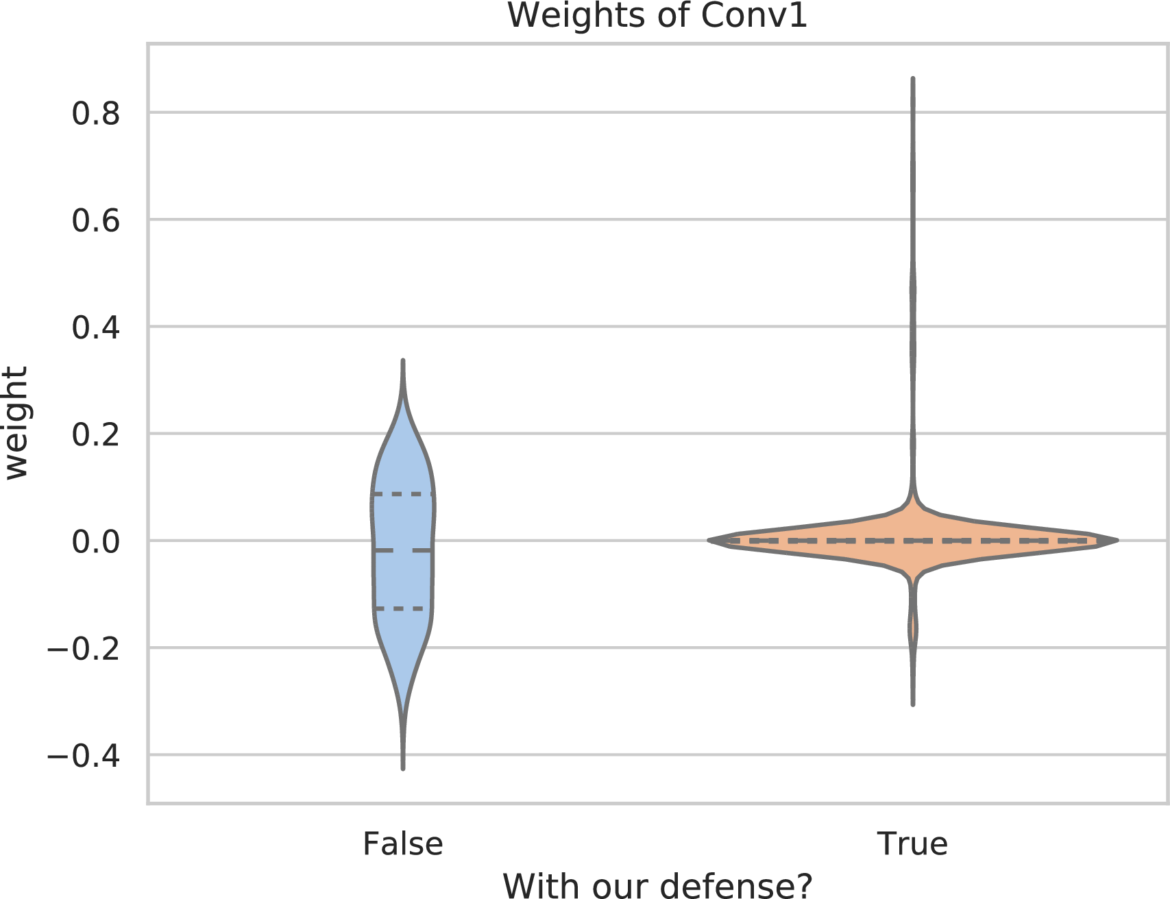
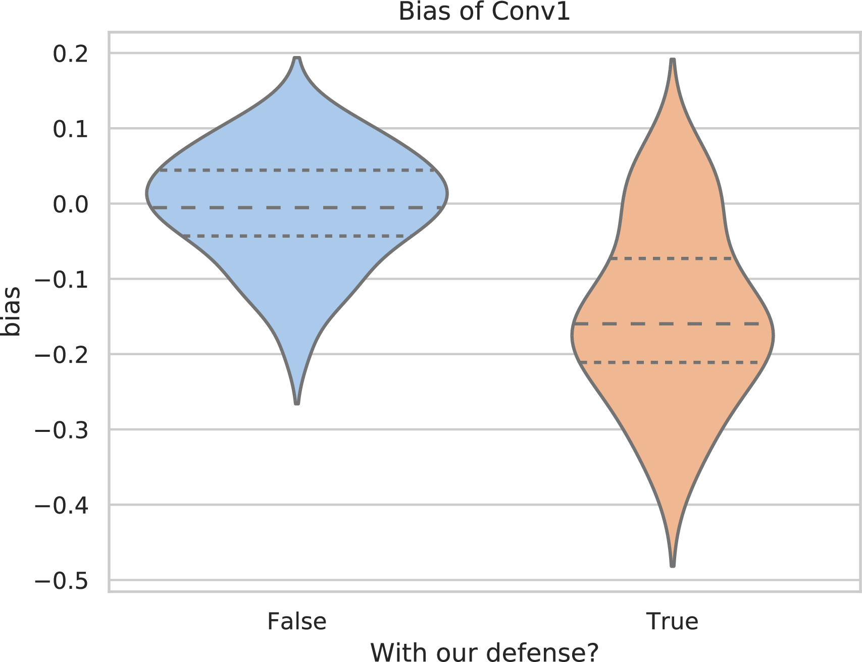
Figure 28: Weights and bias of the first convolutional layer (conv1) with/without our defense..
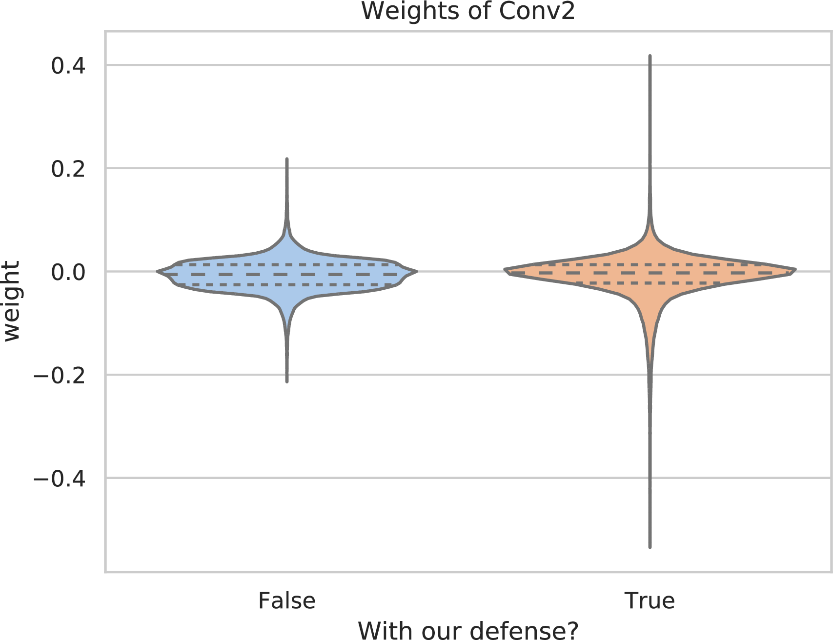
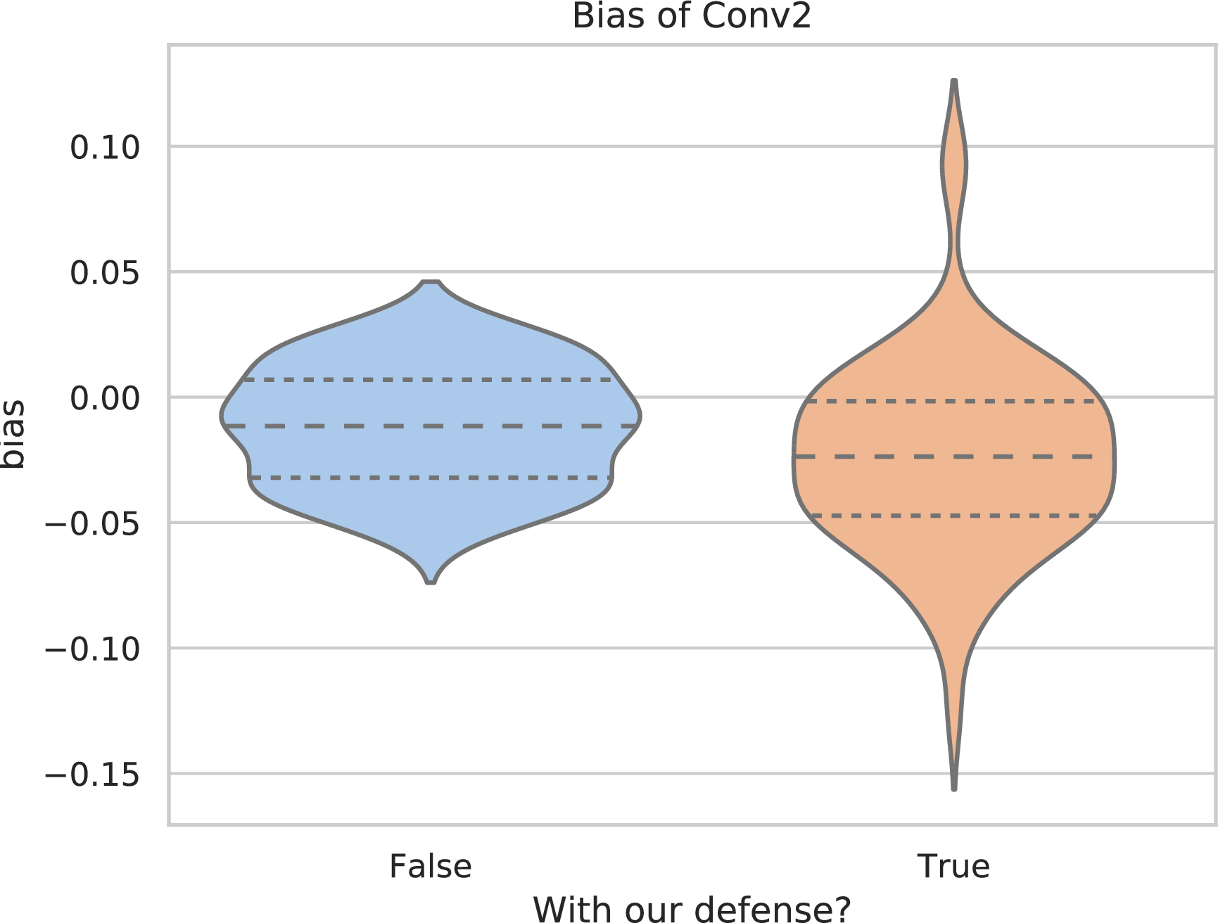
Figure 29: Weights and bias of the second convolutional layer (conv2) with/without our defense..
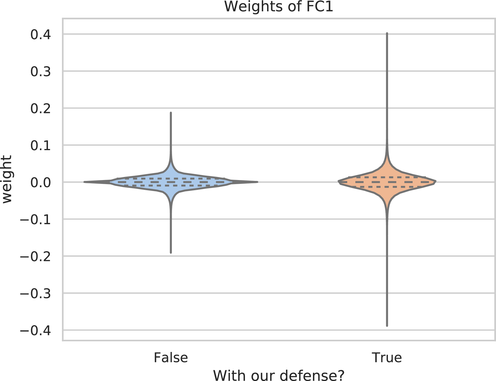
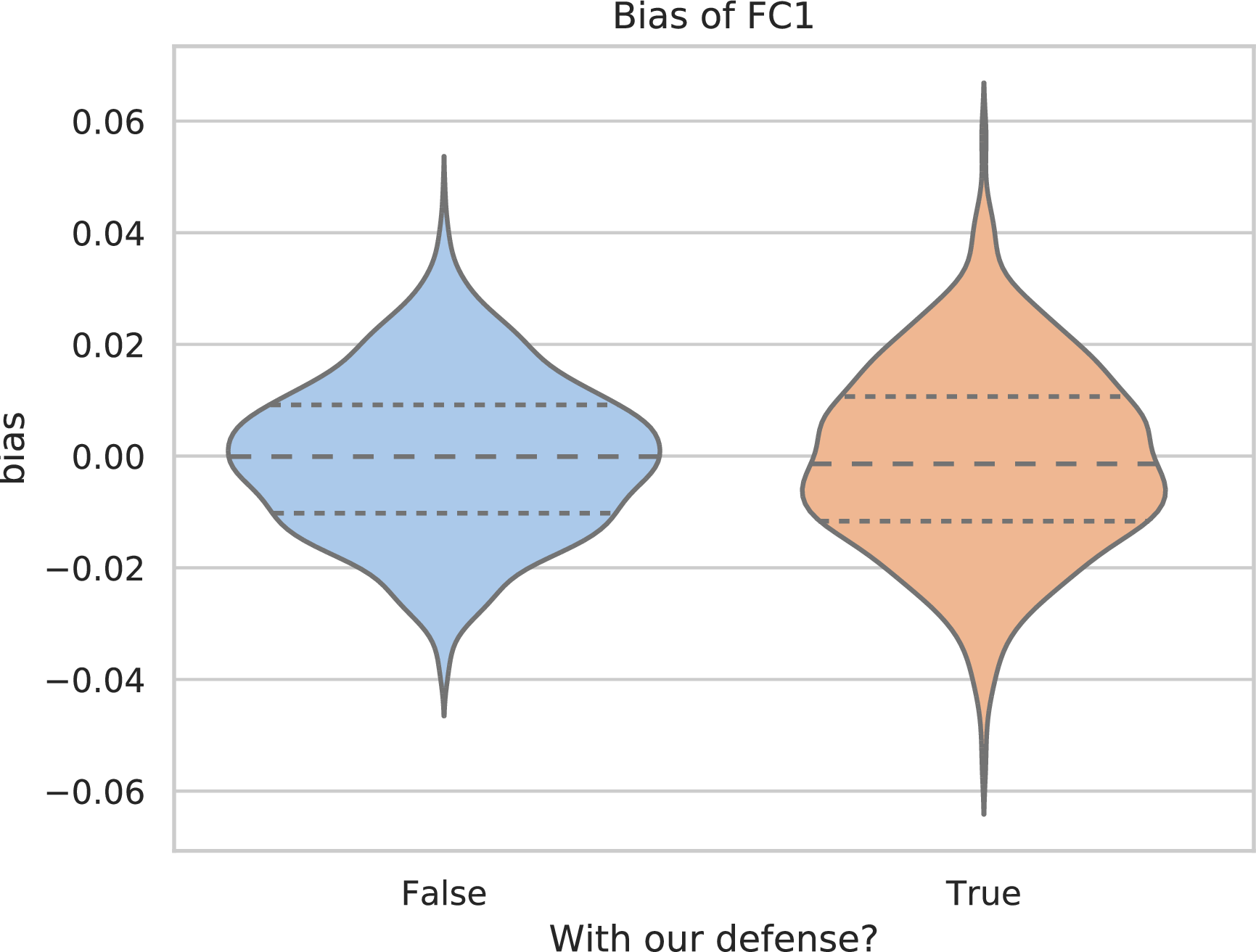
Figure 30: Weights and bias of the first fully-connected layer (fc1) with/without our defense..
Ian [4] proposed a linear explanation of adversarial examples:
Consider the dot product between a weight vector \(w\) and an adversarial example \(\tilde{x}=x+r~(\|r\|_\infty < \varepsilon)\): \[w^T\tilde{x} = w^Tx + w^Tr.\] The adversarial perturbation causes the activation to grow by \(w^Tr\). We can maximize this increase subject to the max norm constraint on \(r\) by assigning \(r=\varepsilon \text{sign}(w)\). If \(w\) has \(k\) dimensions and the average magnitude of an element of the weight vector is \(h\), then the activation will grow by \(\varepsilon k h\). Since \(\|r\|_\infty\) does not grow with the dimensionality of the problem but the change in activation caused by perturbation by \(r\) can grow linearly with \(k\), then for high dimensional problems, we can make many infinitesimal changes to the input that add up to one large change to the output.
In our experiments, we analysed the parameters in models trained on MNIST, as shown in Fig. 28, 29, 30. These violin plots suggest that
the weights in the first convolution layer of the defensive model are closer to \(0\) and have smaller variance than those of the vanilla model. That means the \(h\) in the above quotation is decreased with our defense, and it will be harder for the \(r\) to incur a large increase in activation \(\varepsilon k h\).
the bias in the first convolution layer of the defensive model tend to be negative values instead of being nearly “zero-mean”. These negative bias could help further suppress the increase in activation caused by purturbation \(r\).
Therefore, Ian ’s [4] theory could explain why our defense works, as the resulting differences in network parameters may help reduce the probability for adversarial perturbation to increase the layer outputs into the local linear area of ReLU.
13 Alternative Attack↩︎
13.1 Distance-based Ranking Attack↩︎
In order to implement the proposed ranking attack, alternative attacking objectives are possible. Some related works such as Feature Adversary [25] generates untargeted adversarial examples against classifiers by maximizing the distance shift of representation vectors off their original locations. This may inspire an alternative version of CA or QA objective functions which are directly based on distance. For example, such alternative objective for CA+ and QA- could be as follows: \[\begin{align} r&=\mathop{\mathrm{arg\,min}}_{r\in\Gamma}\sum_{q\in Q}d(q,c+r)\\ r&=\mathop{\mathrm{arg\,max}}_{r\in\Gamma}\sum_{c\in C}d(q+r,c). \end{align}\] However, it must be pointed out that our method significantly differs from feature adversary [25]: (1) Feature adversary concerns the pairwise similarity of source-target representations, while our image ranking problem concerns the ranking order of multiple candidates; (2) Feature adversary attempts to reduce the \(\ell_2\) distance as much as possible, while our triplet-like loss attempts to make positive candidates closer to query than the negative ones, which well fits the objective of ranking order optimization. Such relative distance optimization becomes more important since our attack simultaneously involves multiple queries and multiple candidates; (3) The \(\ell_2\) distance based methods suffer from inevitable disadvantages. Specifically, distance-based objectives are suboptimal, because they disregard the relative positions among the candidates and queries.
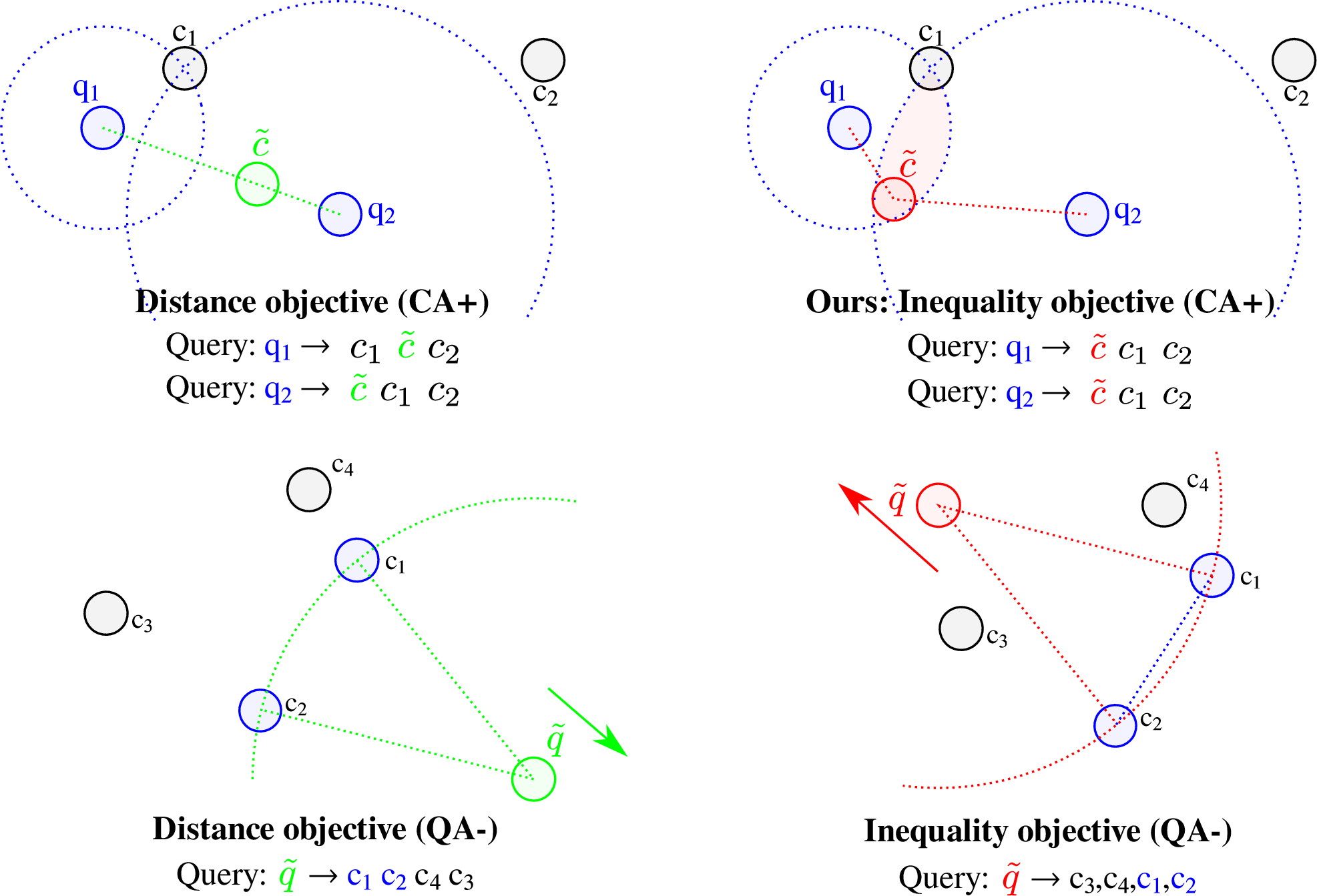
As shown in the top-left part of Fig. 31, the solution set for for distance-based CA+ (the green dotted line) contains suboptimal solutions. Similarly, in the bottom-left part of Fig. 31 the distance-based objective for QA- tends to maximize the sum of distance neglecting the ranking result, and further optimization (moving \(\tilde{q}\) along the green arrow) will not change the ranking result. In contrast, our proposed inequality-based method does not suffer from these issues, as shown in the top-right and bottom-right parts.
We also implemented such distance-based method and compared it with our triplet-like method, as shown in Tab. 14. Experimental results suggest that our method always outperforms distance-based method by a margin. Especially for QA-, the distance-based objective is very difficult to optimize because the distance-based Semantics-Preserving term contradicts with the other term in the loss function. In summary, distance-based method is not well-suited for our proposed adversarial ranking attack, especially in the scenario of QA-.
| \(\varepsilon\) | CA+ | CA- | QA+ | QA- | ||||||||||||
| \(w=1\) | \(2\) | \(5\) | \(10\) | \(w=1\) | \(2\) | \(5\) | \(10\) | \(m=1\) | \(2\) | \(5\) | \(10\) | \(m=1\) | \(2\) | \(5\) | \(10\) | |
| 0.3 | 3.0 | 9.5 | 15.9 | 22.2 | 86.0 | 85.2 | 84.7 | 84.6 | 7.4 | 20.2 | 34.9 | 41.7 | 0.8 | 0.8 | 0.8 | 0.8 |
14 Alternative Defense↩︎
Apart from the defense provided in the manuscript, we also tried some other loss functions for adversarial training. In literature, there is no predominant choice for the adversarial training loss function. The only common trait among these choices is that all of them involve adversarial examples. Inspired by previous works, we also implement some alternative defenses for ranking systems as follows.
14.1 Straightforward Adaptation of Madry Defense↩︎
Madry [18] formularised improving neural network classifier robustness as a min-max optimization problem, where the inner maximization seeks to generate adversarial examples that lead to maximum cross-entropy loss \(L_\text{CE}\), while the outer minimization tunes the neural network parameters \(\theta\) to suppress the cross-entropy loss: \[\min_\theta \Big\{ \mathbb{E}_{(x,y)\sim D} \big[ \max_{r\in\Gamma} L_\text{CE} (x+r,y) \big] \Big\}\] where \((x,y)\) is a pair of image and ground-truth class label.
Similarly, we follow the idea and use a similar defense for ranking models: \[\min_\theta \Big\{ \mathbb{E}_{(q,c_p,c_n)\sim D} \big[ \max_{r\in\Gamma}L_{\text{triplet}}(q+r,c_p,c_n) \big] \Big\} \label{eq:mintmaxt}\tag{14}\] where the inner maximization aims to generate strongest adversarial examples that could lead to triplet ranking error and a large loss value, while the outer minimization seeks network parameters that could reduce such error.
However, during experiments, we observe that such defensive loss function always diverges, possibly due to the adversarial examples generated by the inner problem being too “strong”. We leave further investigation into this problem for future work.
14.2 Straightforward Adaptation of Ian Defense↩︎
Ian [4] proposed the following loss function for adversarial training: \[\begin{align} L_\text{Ian}(x, y) &= \alpha L_\text{CE}(x,y) \\ &+ (1-\alpha)L_\text{CE}(x + \varepsilon \text{sign}(\nabla_x L_\text{CE} (x,y) )) \end{align}\] where the first term is a normal Cross-Entropy loss, and the second term is the cross-entropy loss with untargeted adversarial example that aims to increase the loss value. Constant \(\alpha\) is a balancing parameter.
When adapted to a deep ranking system, this defense method also suffers from the diverging issue similar to Madry’s defense.
| \(\varepsilon\) | CA+ | CA- | QA+ | QA- | ||||||||||||
| \(w=1\) | \(2\) | \(5\) | \(10\) | \(w=1\) | \(2\) | \(5\) | \(10\) | \(m=1\) | \(2\) | \(5\) | \(10\) | \(m=1\) | \(2\) | \(5\) | \(10\) | |
| 0 | 50 | 50 | 50 | 50 | 1.2 | 1.2 | 1.2 | 1.2 | 50 | 50 | 50 | 50 | 0.5 | 0.5 | 0.5 | 0.5 |
| 0.01 | 49.1 | 49.3 | 49.6 | 49.5 | 1.3 | 1.3 | 1.3 | 1.3 | 49.7, 0.0 | 49.9, 0.0 | 50.0, 0.0 | 49.8, 0.0 | 0.5, 0.0 | 0.5, 0.0 | 0.5, 0.0 | 0.5, 0.0 |
| 0.03 | 48.0 | 48.2 | 48.5 | 48.6 | 1.6 | 1.5 | 1.5 | 1.5 | 48.7, 0.0 | 49.2, 0.0 | 49.7, 0.0 | 49.7, 0.0 | 0.6, 0.0 | 0.5, 0.0 | 0.5, 0.0 | 0.5, 0.0 |
| 0.1 | 43.1 | 44.4 | 45.2 | 45.5 | 2.4 | 2.3 | 2.1 | 2.1 | 45.3, 0.1 | 47.4, 0.1 | 48.6, 0.1 | 49.4, 0.1 | 0.8, 0.1 | 0.7, 0.1 | 0.6, 0.1 | 0.6, 0.1 |
| 0.3 | 33.3 | 35.8 | 37.4 | 38.0 | 5.6 | 5.1 | 4.8 | 4.7 | 38.2, 0.3 | 42.3, 0.3 | 45.7, 0.3 | 47.6, 0.3 | 2.1, 0.4 | 1.7, 0.4 | 1.5, 0.4 | 1.5, 0.4 |
| 0 | 50 | 50 | 50 | 50 | 1.5 | 1.5 | 1.5 | 1.5 | 50 | 50 | 50 | 50 | 0.5 | 0.5 | 0.5 | 0.5 |
| 0.01 | 49.3 | 49.6 | 49.5 | 49.7 | 1.6 | 1.6 | 1.6 | 1.6 | 49.5, 0.0 | 49.7, 0.0 | 50.0, 0.0 | 50.0, 0.0 | 0.5, 0.0 | 0.5, 0.0 | 0.5, 0.0 | 0.5, 0.0 |
| 0.03 | 48.2 | 48.3 | 48.8 | 48.8 | 1.8 | 1.8 | 1.8 | 1.7 | 49.3, 0.0 | 48.9, 0.0 | 49.5, 0.0 | 49.7, 0.0 | 0.6, 0.0 | 0.5, 0.0 | 0.5, 0.0 | 0.5, 0.0 |
| 0.1 | 44.7 | 45.4 | 46.3 | 46.4 | 2.8 | 2.6 | 2.5 | 2.5 | 46.3, 0.1 | 47.4, 0.1 | 48.6, 0.1 | 49.2, 0.1 | 0.7, 0.1 | 0.7, 0.1 | 0.6, 0.1 | 0.6, 0.1 |
| 0.3 | 35.5 | 38.5 | 40.3 | 40.9 | 5.7 | 5.3 | 5.1 | 5.0 | 39.3, 0.4 | 43.1, 0.3 | 46.0, 0.3 | 47.5, 0.3 | 1.8, 0.4 | 1.6, 0.4 | 1.4, 0.4 | 1.4, 0.4 |
0.2em
14.3 Directly Suppressing Shift Distance↩︎
As discussed in the manuscript, another possible adversarial training method could be to directly suppress the maximum shift distance of embedding vectors, :
\[L_{\text{trip-es}} = L_{\text{triplet}}(q,c_p,c_n) + \sum_{x\in\{q,c_p,c_n\}} \big(\max_{r\in\Gamma} d(x+r, x)\big), \label{eq:trip-es}\tag{15}\]
where the most severe distance shift incurred by adversarial perturbations is explicitly suppressed, in addition to a standard ranking loss term.
Experimental results (Tab. 15) show that cosine distance-based ranking models are more robust with this defense. However, we note that this loss may numerically explode on an Euclidean distance-based embedding model, as a strong adversary can gradually cause very large embedding shift distance. To mitigate such divergence issue, we also tried to add a balancing parameter to greatly scale down the second term of the loss function, but the instability problem was still not alleviated.
Due to the lack of universality, we leave this alternative defense in supplementary material as a pure discussion, and possible improvements as future work.