Confidence Sets and Hypothesis Testing in a Likelihood-Free Inference Setting
February 24, 2020
Abstract
Parameter estimation, statistical tests and confidence sets are the cornerstones of classical statistics that allow scientists to make inferences about the underlying process that generated the observed data. A key question is whether one can still
construct hypothesis tests and confidence sets with proper coverage and high power in a so-called likelihood-free inference (LFI) setting; that is, a setting where the likelihood is not explicitly known but one can forward-simulate observable data
according to a stochastic model. In this paper, we present ACORE (Approximate Computation via Odds Ratio Estimation), a frequentist approach to LFI that first formulates the classical likelihood ratio test (LRT) as a parametrized
classification problem, and then uses the equivalence of tests and confidence sets to build confidence regions for parameters of interest. We also present a goodness-of-fit procedure for checking whether the constructed tests and confidence regions are
valid. ACORE is based on the key observation that the LRT statistic, the rejection probability of the test, and the coverage of the confidence set are conditional distribution functions which often vary smoothly as a function of the parameters
of interest. Hence, instead of relying solely on samples simulated at fixed parameter settings (as is the convention in standard Monte Carlo solutions), one can leverage machine learning tools and data simulated in the neighborhood of a parameter to
improve estimates of quantities of interest. We demonstrate the efficacy of ACORE with both theoretical and empirical results. Our implementation is available on Github.
1 Introduction↩︎
Parameter estimation, statistical tests and confidence sets are the cornerstones of classical statistics that relate observed data to properties of the underlying statistical model. Most frequentist procedures with good statistical performance (e.g., high power) require explicit knowledge of a likelihood function. However, in many science and engineering applications, complex phenomena are modeled by forward simulators that implicitly define a likelihood function: For example, given input parameters \(\theta\), a statistical model of our environment, climate or universe may combine deterministic dynamics with random fluctuations to produce synthetic data \(\mathbf{X}\). Simulation-based inference without an explicit likelihood is called likelihood-free inference (LFI).
The literature on LFI is vast. Traditional LFI methods, such as Approximate Bayesian Computation (ABC; [1]–[3]), estimate posteriors by using simulations sufficiently close to the observed data, hence bypassing the likelihood. More recently, several approaches that leverage machine learning algorithms have been proposed; these either directly estimate the posterior distribution [4]–[7] or the likelihood function [8]–[13]. We refer the reader to [14] for a recent review of the field.
A question that has not received much attention so far is whether one, in an LFI setting, can construct inference techniques with good frequentist properties. Frequentist procedures have nevertheless played an important role in many fields. In high energy physics for instance, classical statistical techniques (e.g., hypothesis testing for outlier detection) have resulted in discoveries of new physics and other successful applications [15]–[17]. Even though controlling type I error probabilities is important in these applications, most LFI methods do not have guarantees on validity or power. Ideally, a unified LFI approach should
be computationally efficient in terms of the number of required simulations,
handle high-dimensional data from different sources (without, e.g., predefined summary statistics),
produce hypothesis tests and confidence sets that are valid; that is, have the nominal type I error or confidence level,
produce hypothesis tests with high power or, equivalently, confidence sets with a small expected size,
provide diagnostics for checking empirical coverage or for checking how well the estimated likelihood fits simulated data.
In this paper, we present ACORE (Approximate Computation via Odds Ratio Estimation), a frequentist approach to LFI, which addresses the above mentioned concerns.
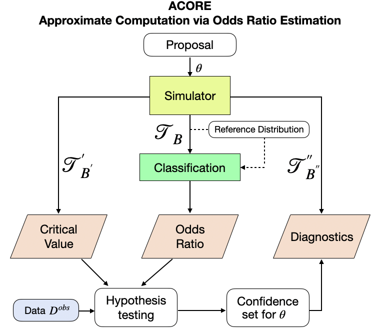
Figure 2 summarizes the ACORE work structure: ACORE first compares synthetic data from the simulator \(F_\theta\) to a reference distribution \(G\) by computing an “Odds Ratio”. The odds ratio can be learnt with a probabilistic classifier, such as a neural network with a softmax layer, suitable for the data at hand. As we shall see, the estimated odds ratio is an
approximation of the likelihood ratio statistic (Proposition [prop::consistency]). The ACORE test statistic (Equation 4 ), together with an estimate of the “Critical Value” (Algorithms 3 and 4), can be used for hypothesis testing or for
finding a confidence set for \(\theta\). ACORE also includes “Diagnostics” (Section 3.3) for computing the empirical coverage of the constructed confidence set for \(\theta\).
At the heart of ACORE is the key observation that the likelihood ratio statistic, the critical value of the test, and the coverage of the confidence set are conditional distribution functions which often vary smoothly as a function of the
(unknown) parameters of interest. Hence, instead of relying solely on samples simulated at fixed parameter settings (as is the convention in standard Monte Carlo solutions), one can leverage machine learning tools and data simulated in the neighborhood of
a parameter to improve estimates of quantities of interest and decrease the total number of simulated data points. Our contribution is three-fold:
a new procedure for estimating the likelihood ratio statistic, which uses probabilistic classifiers and does not require repeated sampling at each \(\theta\) or a separate interpolation or calibration step;
an efficient procedure for estimating the critical value that guarantees valid tests and confidence sets, based on quantile regression without repeated sampling at each \(\theta\);
a new goodness-of-fit technique for computing empirical coverage of constructed confidence sets as a function of the unknown parameters \(\theta\).
Finally, ACORE is simple and modular by construction. One can easily switch out, generalize or take pieces of the framework and apply it to any similar machine-learning-based LFI setting. The theoretical results of Section 3.1 hold for a general setting. In addition, given the vast arsenal of existing probabilistic classifiers developed in the literature, ACORE can be applied to many different types of complex data
\({\mathbf{X}}\) (e.g., images, time series and functional data). In Section 4, we show empirical results connecting the power of the constructed hypothesis tests to the performance
of the classifier. Note also that Algorithms 3 and 4 for estimating parametrized critical values apply to any hypothesis test on \(\theta\) of the form of Equation 2 for any test statistic \(\tau\). The goodness-of-fit procedure in Section 3.3
for checking empirical coverage as a function of \(\theta\) is also not tied to odds ratios.
1.1 Related Work↩︎
The problem of constructing confidence intervals with good frequentist properties has a long history in statistics [15], [18], [19]. One of the earlier simulation-based approaches was developed in high energy physics (HEP) by [20]; their proposed scheme of estimating the likelihood and likelihoood ratio statistic nonparametrically by histograms of photon counts would later become a key component in the discovery of the Higgs Boson [21]. However, traditional approaches for building confidence regions and hypothesis tests in LFI rely on a series of Monte Carlo samples at each parameter value \(\theta\) [22]–[24]. Thus, these approaches quickly become inefficient with large or continuous parameter spaces. Traditional nonparametric approaches also have difficulties handling high-dimensional data without losing key information.
LFI has recently benefited from using powerful machine learning tools like deep learning to estimate likelihood functions and likelihood ratios for complex data. Successful application areas include HEP [25], astronomy [26] and
neuroscience [27]. ACORE has some similarities to the work of [28] which also uses machine learning methods for frequentist inference in an LFI setting. Other elements of ACORE such as leveraging the
ability of ML algorithms to smooth over parameter space turning a density ratio estimate into a supervised classification problem have also previously been used in LFI settings: Works that smooth over parameter space include, e.g., Gaussian processes [29], [30] and neural networks [31]. Works that turn a density ratio into a classification problem include applications to generative models (see [32] for a review), and Bayesian LFI [9], [33]–[35]. Finally, like ACORE, [36] explores frequentist guarantees of confidence
regions; however those regions are built under a Bayesian framework.
Novelty. What distinguishes the ACORE approach from other related work is that it uses an efficient procedure for estimating the (i) likelihood ratio, (ii) critical values and (iii) coverage of confidence sets across the
entire parameter space, without the need for an extra interpolation or calibration step (as in traditional Monte Carlo solutions and more recent ML approaches). To the best of our knowledge, (ii) and (iii) are entirely novel in the LFI literature. In
contrast to other methods that estimate (i), ACORE does not make parametric assumptions or require an additional calibration step, and it can accommodate all types of hypotheses. We provide theoretical guarantees on our procedures in terms of
power and validity (Section 3.1; proofs in Supplementary Material 9). We also offer a scheme for how to choose ML algorithms and the number of simulations so as to have
good power properties and valid inference in practice.
Notation. Let \(F_{\theta}\) with density \(f_\theta\) represent the stochastic forward simulator for a sample point \({\mathbf{X}}\in \mathcal{X}\) at parameter \(\theta \in \Theta\). We denote i.i.d “observable” data from \(F_{\theta}\) by \({\mathcal{D}}=\left\{ {\mathbf{X}}_1^{\text{obs}},\ldots,{\mathbf{X}}_n^{\text{obs}} \right\}\), and the actually observed or measured data by \(D=\left\{ {\mathbf{x}}_1^{\text{obs}},\ldots,{\mathbf{x}}_n^{\text{obs}} \right\}\). The likelihood function \({\mathcal{L}}({\mathcal{D}};\theta)=\prod_{i=1}^{n} f_\theta({\mathbf{X}}_i^{\text{obs}})\).
2 Statistical Inference in a Traditional Setting↩︎
We begin by reviewing elements of traditional statistical inference that play a key role in ACORE.
Equivalence of tests and confidence sets. A classical approach to constructing a confidence set for an unknown parameter \(\theta \in \Theta\) is to invert a series of hypothesis tests [18]: Suppose that for each possible value \(\theta_0 \in \Theta\), there is a level \(\alpha\) test \(\delta_{\theta_0}\) of \[H_{0, \theta_0}: \theta=\theta_0 \;\;versus \;\;H_{1, \theta_0}: \theta \neq \theta_0; \label{eq:test95Neyman}\tag{1}\] that is, a test \(\delta_{\theta_0}\) where the type I error (the probability of erroneously rejecting a true null hypothesis \(H_{0, \theta_0}\)) is no larger than \(\alpha\). For observed data \({\mathcal{D}}=D\), now define \(R(D)\) as the set of all parameter values \(\theta_0 \in \Theta\) for which the test \(\delta_{\theta_0}\) does not reject \(H_{0,\theta_0}\). Then, by construction, the random set \(R({\mathcal{D}})\) satisfies \[\mathbb{P}\left[\theta_0 \in R({\mathcal{D}}) \;\middle\vert \;\theta=\theta_0\right] \geq 1-\alpha\] for all \(\theta_0 \in \Theta\). That is, \(R({\mathcal{D}})\) defines a \((1-\alpha)\) confidence set for \(\theta\). Similarly, we can define a test with a desired significance level from a confidence set with a certain coverage.
Likelihood ratio test. A general form of hypothesis tests that often leads to high power is the likelihood ratio test (LRT). Consider testing \[\label{eq:hypothesis95testing} H_0: \theta \in \Theta_0 \;\;versus \;\;H_1: \theta \in \Theta_1,\tag{2}\] where \(\Theta_1=\Theta \setminus \Theta_0\). For the likelihood ratio (LR) statistic, \[\label{eq::LRT} \Lambda({\mathcal{D}}; \Theta_0) = \log \frac{\sup_{\theta \in \Theta_0}{\mathcal{L}}({\mathcal{D}};\theta)}{\sup_{\theta \in \Theta}{\mathcal{L}}({\mathcal{D}};\theta)},\tag{3}\] the LRT of hypotheses (2 ) rejects \(H_0\) when \(\Lambda(D; \Theta_0) < C\) for some constant \(C\).
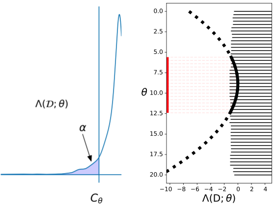
Figure 1 illustrates the construction of confidence sets for \(\theta\) from level \(\alpha\) likelihood ratio tests (1 ). The critical value for each such test \(\delta_{\theta_0}\) is \(C_{\theta_0} = \left\{C: \mathbb{P}\left[\Lambda({\mathcal{D}}; \theta_0)< C \mid \theta=\theta_0 \right] = \alpha \right\}.\)
3 ACORE: Approximate Computation via Odds Ratio Estimation↩︎
In a likelihood-free inference setting, we cannot directly evaluate the likelihood ratio statistic. Here we describe the details of how a simulation-based approach (ACORE, Figure 2) can lead to
hypothesis tests and confidence sets with good frequentist properties.
3.1 Hypothesis Testing via Odds Ratios↩︎
We start by simulating a labeled sample for computing odds ratios. The estimated odds ratio then defines a new test statistic that we use in place of the unknown likelihood ratio statistic.
Simulating a labeled sample. Let \(G\) be a distribution with larger support than \(F_\theta\) for all \(\theta \in \Theta\). The distribution \(G\) could for example be a dominating distribution which it is easy to sample from. We use \(F_{\theta}\) and \(G\) to simulate a labeled training sample \(T_B = \{\theta_i,{\mathbf{x}}_i,y_i\}_{i=1}^B\) for estimating odds ratios. The random sample \({\mathcal{T}}_B= \{\theta_i,{\mathbf{X}}_i,Y_i\}_{i=1}^B\) is identically distributed as \((\theta,{\mathbf{X}},Y)\), where the parameters \(\theta \sim r_{\Theta}\) (a fixed proposal distribution over \(\Theta\)), the “label” \(Y \sim \text{Ber}(p)\) (a Bernoulli distribution with known \(p\) with \(Y\) independent of \(\theta\)), \({\mathbf{X}}|\theta,Y=1\sim F_{\theta}\) and \({\mathbf{X}}|\theta,Y=0\sim G\). That is, the label \(Y_i\) is the indicator that the sample point \({\mathbf{X}}_i\) was generated from \(F_\theta\) rather than \(G\). We call \(G\) a “reference distribution” as we are comparing \(F_\theta\) for different \(\theta\) with this distribution. For all our experiments in this work we use p=1/2; other choices could account for computational differences in sampling from \(F_\theta\) versus \(G\). (Algorithm 7 in Supplementary Material 7 summarizes our procedure.)
Odds ratios. For fixed \({\mathbf{x}}\), we define the odds at \(\theta\) as \[{\mathbb{O}}({\mathbf{x}};\theta):=\frac{\mathbb{P}(Y=1|\theta,{\mathbf{x}})}{\mathbb{P}(Y=0|\theta,{\mathbf{x}})},\] and the odds ratio at \(\theta_0,\theta_1 \in \Theta\) as \[\mathbb{OR}({\mathbf{x}};\theta_0,\theta_1):= \frac{\mathbb{O}(\theta_0;{\mathbf{x}})}{\mathbb{O}(\theta_1;{\mathbf{x}})}.\] One way of interpreting the odds \({\mathbb{O}}(\theta,{\mathbf{X}})\) is to regard it as a measure of the chance that \({\mathbf{X}}\) was generated from \(F_\theta\). That is, a large odds \({\mathbb{O}}(\theta,{\mathbf{x}})\) reflects the fact that it is plausible that \({\mathbf{x}}\) was generated from \(F_\theta\) (rather than \(G\)). Thus, \(\mathbb{OR}({\mathbf{x}};\theta_0,\theta_1)\) measures the plausibility that \({\mathbf{x}}\) was generated from \(\theta_0\) rather than \(\theta_1\). When testing (2 ), we therefore reject \(H_0\) if \(\sup_{\theta_0 \in \Theta_0}\inf_{\theta_1 \in \Theta} \sum_{i=1}^n \log \left( \mathbb{OR}({\mathbf{X}}_i^{\text{obs}};\theta_0,\theta_1)\right) < C\), for some constant \(C\). By Bayes rule, this is just the likelihood ratio test of (2 ).
Hypothesis testing in an LFI setting. In an LFI setting, we cannot directly evaluate the likelihood ratio statistic (3 ). The advantage of rewriting the LRT in terms of odds ratios is that we can forward-simulate a labeled training sample \(\mathcal{D}_B\), as described above, and then use a probabilistic classifier (suitable for the data at hand) to efficiently estimate the odds ratios \(\mathbb{OR}({\mathbf{x}};\theta_0,\theta_1)\) for all \(\theta_1, \theta_2 \in \Theta\): The probabilistic classifier compares data from the forward simulator \(F_\theta\) with data from the reference distribution \(G\) and returns a parametrized odds estimate \(\widehat{\mathbb{O}}({\mathbf{x}}; \theta)\), which is a function of \(\theta \in \Theta\). We can directly compute the odds ratio estimate \(\widehat{\mathbb{OR}}({\mathbf{x}}; \theta_0,\theta_1)\) at any two values \(\theta_1, \theta_2 \in \Theta\) from \(\widehat{\mathbb{O}}({\mathbf{x}}; \theta)\). There is no need for a separate training step.
We reject \(H_0\) if the ACORE test statistic defined as \[\begin{align}
\label{eq:odds95ratio95statistic} \tau({\mathcal{D}}; \Theta_0):=\sup_{\theta_0 \in \Theta_0} \;\inf_{\theta_1 \in \Theta} \sum_{i=1}^n \log \left( \widehat{\mathbb{OR}}({\mathbf{X}}_i^{\text{obs}};\theta_0,\theta_1)\right)
\end{align}\tag{4}\] is small enough for observed data \({\mathcal{D}}=D\). If the probabilities learned by the classifier are well estimated, \(\tau\) is exactly the
likelihood ratio statistic:
If \(\;\widehat{\mathbb{P}}(Y=1|\theta,{\mathbf{x}})=\mathbb{P}(Y=1|\theta,{\mathbf{x}})\) for every \(\theta\) and
\({\mathbf{x}}\), then the ACORE test statistic (4 ) is the likelihood ratio statistic (Equation 3 ).
Estimating the critical value. A key question is how to efficiently estimate the critical value of a test. In this section we consider a single composite null hypothesis \(H_0:\theta \in \Theta_0\). (The setting for constructing confidence sets by testing (1 ) for all \(\theta_0 \in \Theta\) is discussed in Section 3.2.). Suppose that we reject the null hypothesis if the test statistic (4 ) is smaller than some constant \(C\). To achieve a test with a desired level of significance \(\alpha\), we need (for maximum power) the largest \(C\) that satisfies \[\label{eq:significance95level} \sup_{\theta \in \Theta_0} \mathbb{P}\left(\tau({\mathcal{D}}; \Theta_0) < C \mid \theta \right) \leq \alpha .\tag{5}\] However, we cannot explicitly compute the critical value \(C\) or the rejection probability as we do not know the distribution of the test statistic \(\tau\).
Simulation-based approaches are often used to compute rejection probabilities and critical values in lieu of large-sample theory approximations. Typically, such simulations compute a separate Monte Carlo simulation at each fixed \(\theta \in \Theta_0\) on, e.g., a fine enough grid on \(\theta\). That is, the convention is to rely solely on sample points generated at fixed \(\theta\) to
estimate the rejection probabilities \(\mathbb{P}(\tau(\mathcal{D};\Theta_0)< C|\theta)\). Here we propose to estimate the critical values \(C\) for all \(\theta
\in \Theta_0\) and significance levels \(\alpha \in [0,1]\) simultaneously. At the heart of our approach is the key observation that the rejection probability \(\mathbb{P}(\tau(\mathcal{D};\Theta_0)< C|\theta)\) is a conditional cumulative distribution function, which in many settings varies smoothly as a function of \(\theta\) and \(C\). Thus, similar to how we estimate odds for the ACORE statistic, one can use data generated in the neighborhood of \(\theta\) to improve estimates of our quantities of interest
at any \(\theta\). This is what a quantile regression implicitly does to estimate \(C\).
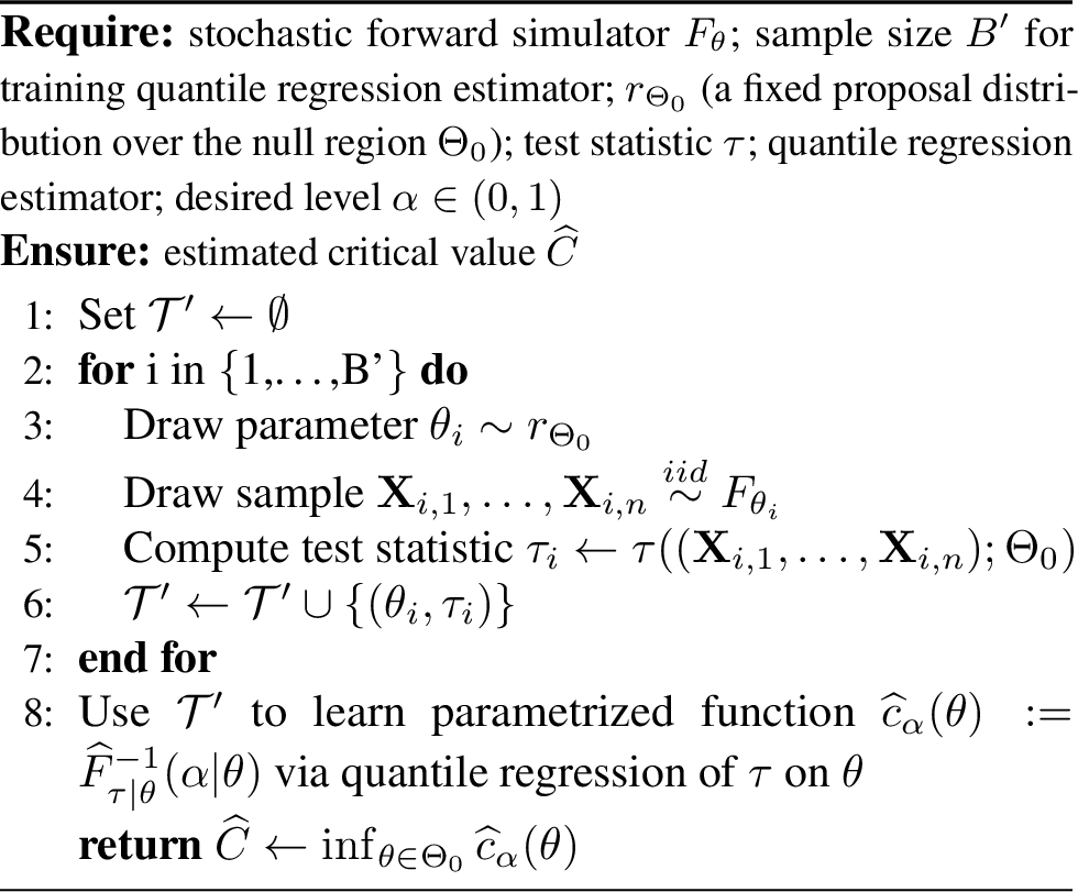
Algorithm 3 outlines the details of the procedure for estimating \(C\). In brief, we use a training sample \({\mathcal{T}}'_{B'}=\{(\theta_i, \tau_i) \}_{i=1}^{B'}\) (independent of \({\mathcal{T}}_B\)) to estimate the \(\alpha\)-conditional quantile \(c_\alpha(\theta)\) defined by \(\mathbb{P}\left(\tau \leq c_\alpha(\theta) \mid \theta \right) = \alpha.\) Let \(\widehat{c}_\alpha(\theta)\) be the estimate of \(c_\alpha(\theta)\) from a quantile regression of \(\tau\) on \(\theta\). By (5 ), our estimate of the critical value \(C\) is \(\widehat{C} = \inf_{\theta \in \Theta_0} \widehat{c}_\alpha(\theta).\) As we shall see, even if the odds are not well estimated, tests and confidence regions based on estimated odds are still valid as long as the thresholds are well estimated. Next we show that the sample size \(B'\) in Algorithm 3 controls the type I error (Theorem 1), whereas the training sample size \(B\) for estimating odds is related to the power of the test (Theorem 2).
Theoretical guarantees. We denote convergence in probability and in distribution by \(\overset{\mathbb{P}}{\rightarrow}\) and \(\xrightarrow[]{\enskip \small Dist \enskip}\), respectively. We start by showing that our procedure leads to valid hypothesis tests (that is, tests that control the type I error probability) as long as \(B'\) in Algorithm 3 is large enough. In order to do so, we assume that the quantile regression estimator used in Algorithm 3 to estimate the critical values is consistent in the following sense:
Assumption 1. Let \(\hat{F}_{B'}(\cdot|\theta)\) be the estimated cumulative distribution function of the test statistic \(\tau\) conditional on \(\theta\) based on a sample size \(B'\), and let \(F(\cdot|\theta)\) be true conditional distribution. For every \(\theta \in \Theta_0\), assume that the quantile regression estimator is such that \[\sup_{t \in \mathbb{R}}|\hat{F}_{B'}(t|\theta)- F(t|\theta)|\xrightarrow[B' \longrightarrow\infty]{\enskip \mathbb{P}\enskip} 0\]
Under some conditions, Assumption 1 holds for instance for quantile regression forests [37].
Next we show that, for every fixed training sample size \(B\) in Algorithm 7, Algorithm 3 yields a valid hypothesis test as \(B' \rightarrow \infty\). The result holds even if the likelihood ratio statistic is not well estimated.
Theorem 1. Let \(C_{B,B'} \in \mathbb{R}\) be the critical value of the test based on the statistic \(\tau=\tau_B\) for a training sample size \(B\) with critical value chosen according to Algorithm 3 for a fixed \(\alpha \in (0,1)\). If the quantile estimator satisfies Assumption 1 and \(|\Theta|<\infty\), then \[C_{B,B'} \xrightarrow[B' \longrightarrow\infty]{\enskip \mathbb{P}\enskip} C_B^*,\] where \(C_B^*\) is such that \[\sup_{\theta \in \Theta_0}\mathbb{P}(\tau_B \leq C_B^*|\theta) = \alpha.\]
Finally we show that as long as the probabilistic classifier is consistent and the critical values are well estimated (which holds for large \(B'\) according to Theorem 1), the power of the ACORE test converges to the power of the LRT as \(B\) grows.
Theorem 2. Let \(\widehat{\phi}_{B,C_B}(\mathcal{D})\) be the test based on the statistic \(\tau=\tau_B\) for a labeled sample size \(B\) with critical value \(C_B \in \mathbb{R}\).1 Moreover, let \(\phi_{C^*}(\mathcal{D})\) be the likelihood ratio test with critical value \(C^* \in \mathbb{R}\).2 If, for every \(\theta \in \Theta\), \[\widehat{\mathbb{P}}(Y=1|\theta,{\mathbf{X}}) \xrightarrow[B \longrightarrow\infty]{\enskip \mathbb{P}\enskip} \mathbb{P}(Y=1|\theta,{\mathbf{X}}),\] where \(|\Theta|<\infty\), and \(\widehat{C}_B\) is such that \(\widehat{C}_B \xrightarrow[B \longrightarrow\infty]{\enskip Dist \enskip}C^*\), then, for every \(\theta \in \Theta\), \[\mathbb{P}\left(\widehat{\phi}_{B,\widehat{C}_B}(\mathcal{D})=1|\theta \right) \xrightarrow[B \longrightarrow\infty]{} \mathbb{P}\left(\phi_{C^*}(\mathcal{D})=1|\theta\right).\]
3.2 Confidence Sets↩︎
To construct a confidence set for \(\theta\), we use the equivalence of tests and confidence sets (Section [sec::trad95inference]): Suppose that we for every \(\theta_0 \in \Theta\) can find the critical value \(C_{\theta_0}\) of a test of (1 ) with type I error no larger than \(\alpha\). The random set \[R({\mathcal{D}}) = \left\{ \theta_0 \in \Theta \;\middle\vert \tau({\mathcal{D}};\theta_0) \geq C_{\theta_0}\right\},\] then defines a \((1-\alpha)\) confidence region for \(\theta\).
However, rather than repeatedly running Algorithm 3 for each null hypothesis \(\Theta_0=\{\theta_0\}\) separately, we estimate all critical values \(C_{\theta_0}\) (for different \(\theta_0 \in \Theta\)) simultaneously. Algorithm 4 outlines our procedure. Again, we use quantile regression to
learn a parametrized function \(C_{\theta_0}\). The whole procedure for computing confidence sets via ACORE is summarized in Algorithm 8 in Supplementary Material 8. Theorem 1 implies that the constructed confidence set has the nominal \(1-\alpha\) confidence level as \(B' \rightarrow \infty\). The size of the confidence set depends on the training sample size \(B\) and the classifier.
![Figure 4: [Many Simple Null Hypotheses] Estimate the critical values C_{\theta_0} for a level-\alpha test of H_{0, \theta_0}: \theta = \theta_0 vs. H_{1, \theta_0}: \theta \neq \theta_0 for all \theta_0 \in \Theta simultaneously](/article/2002.10399/_pdflatex/vmahqpio.png "fig:")
3.3 Evaluating Empirical Coverage for All Possible Values of \(\theta\)↩︎
After the parametrized ACORE statistic and the critical values have been estimated, it is important to check whether the resulting confidence sets indeed are valid or, equivalently, if the resulting hypothesis tests have the nominal
significance level. We also want to identify regions in parameter space where we clearly overcover. That is, the two main questions are: (i) do the constructed confidence sets satisfy \[\mathbb{P}\left[\theta_0 \in
R({\mathcal{D}}) \;\middle\vert \;\theta=\theta_0\right] \geq 1-\alpha,\] for every \(\theta_0 \in \Theta\), and (ii) how close is the actual coverage to the nominal confidence level \(1-\alpha\)? To answer these questions, we propose a goodness-of-fit procedure where we draw \(B''\) new samples from the simulator given \(\theta\),
construct a confidence set for each sample, and then check which computed regions include the “true” \(\theta\). More specifically: we generate a set \(\mathcal{T}_{B''}''
=\{(\theta'_1,{\mathcal{D}}'_1),\ldots,(\theta'_{B''},{\mathcal{D}}'_{B''})\}\), where \(\theta_i' \sim r_{\Theta}\) and \({\mathcal{D}}'_i\)
is a sample of size \(n\) of i.i.d. observable data from \(F_{\theta'_i}\). We then define \[W_i:=\mathbb{I}\left(\theta'_i \in
R({\mathcal{D}}'_i)\right),\] where \(R({\mathcal{D}}'_i)\) is the confidence set for \(\theta\) for data \({\mathcal{D}}'_i\). If \(R\) has the correct coverage, then \[\mathbb{P}(W_i = 1|\theta_i )\geq 1-\alpha.\] We can estimate the probability \(\mathbb{P}(W_i = 1|\theta_i )\) using any
probabilistic classifier; some methods also provide confidence bands that assess the uncertainty in estimating this quantity [38]–[40]. By comparing the estimated probability to \(1-\alpha\), we have a diagnostic
tool for checking how close we are to the nominal confidence level over the entire parameter space \(\Theta\). See Figure 5 for an example.
Finally note that our procedure parametrizes the coverage of the confidence set as a function of the true parameter value. This is in contrast to other goodness-of-fit techniques (e.g., [41]–[44]) that only check for marginal coverage, i.e., \(n^{-1}\sum_{i=1}^{n} W_i \geq 1-\alpha\).
4 Toy Examples↩︎
We consider two examples where the true likelihood is known. In the first example, the forward simulator \(F_\theta\) follows a \(\textrm{Poisson}(100 + \theta)\) distribution similar to the signal-background model in Section 5. In the second example, we consider a Gaussian mixture model (GMM) with two unit-variance Gaussians centered at \(-\theta\) and \(\theta\), respectively. In both examples, \(n=10\), the proposal distribution \(r_{\Theta}\) is a uniform distribution, and the reference distribution \(G\) is a normal distribution. Table 1 summarizes the set-up.
| Poisson Example | GMM Example | |
|---|---|---|
| \(r_{\Theta}\) | \({\rm Unif}(0,20)\) | \({\rm Unif}(0,10)\) |
| \(F_\theta\) | \(\Pois(100 + \theta)\) | \(\frac{1}{2}\mathcal{N}(-\theta, 1) + \frac{1}{2}\mathcal{N}(\theta, 1)\) |
| \(G\) | \(\mathcal{N}(110, 15^2)\) | \(\mathcal{N}(0, 5^2)\) |
| True \(\theta\) | \(\theta_0 = 10\) | \(\theta_0 = 5\) |
| Poisson Example | ||||
|---|---|---|---|---|
| \(B\) | Classifier | Cross | Average | Size of |
| Entropy Loss | Power | Confidence Set [%] | ||
| 100 | MLP | 0.87 \(\pm\) 0.27 | 0.24 | 75.9 \(\pm\) 19.3 |
| NN | 0.76 \(\pm\) 0.15 | 0.29 | 71.6 \(\pm\) 19.7 | |
| QDA | 0.66 \(\pm\) 0.02 | 0.41 | 60.0 \(\pm\) 15.6 | |
| 500 | MLP | 0.69 \(\pm\) 0.01 | 0.35 | 65.9 \(\pm\) 20.4 |
| NN | 0.67 \(\pm\) 0.01 | 0.38 | 62.9 \(\pm\) 15.8 | |
| QDA | 0.64 \(\pm\) 0.01 | 0.47 | 54.2 \(\pm\) 9.4 | |
| 1,000 | MLP | 0.69 \(\pm\) 0.01 | 0.37 | 63.3 \(\pm\) 19.8 |
| NN | 0.66 \(\pm\) 0.01 | 0.44 | 56.9 \(\pm\) 15.9 | |
| QDA | 0.64 \(\pm\) 0.01 | 0.50 | 51.3 \(\pm\) 7.7 | |
| - | Exact | 0.64 \(\pm\) 0.01 | 0.54 | 45.0 \(\pm\) 4.9 |
| GMM Example | ||||
|---|---|---|---|---|
| \(B\) | Classifier | Cross | Average | Size of |
| Entropy Loss | Power | Confidence Set [%] | ||
| 100 | MLP | 0.39 \(\pm\) 0.03 | 0.88 | 14.1 \(\pm\) 4.7 |
| NN | 0.81 \(\pm\) 0.31 | 0.42 | 58.4 \(\pm\) 23.3 | |
| QDA | 0.64 \(\pm\) 0.02 | 0.15 | 85.3 \(\pm\) 21.1 | |
| 500 | MLP | 0.35 \(\pm\) 0.01 | 0.90 | 12.1 \(\pm\) 2.4 |
| NN | 0.45 \(\pm\) 0.05 | 0.57 | 44.3 \(\pm\) 24.1 | |
| QDA | 0.62 \(\pm\) 0.01 | 0.15 | 84.9 \(\pm\) 19.9 | |
| 1,000 | MLP | 0.35 \(\pm\) 0.01 | 0.90 | 12.1 \(\pm\) 2.5 |
| NN | 0.41 \(\pm\) 0.02 | 0.77 | 24.9 \(\pm\) 15.9 | |
| QDA | 0.62 \(\pm\) 0.01 | 0.12 | 88.1 \(\pm\) 18.0 | |
| - | Exact | 0.35 \(\pm\) 0.01 | 0.92 | 9.5 \(\pm\) 2.0 |
First we investigate how the power of ACORE and the size of the derived confidence sets depend on the performance of the classifier used in the odds ratio estimation (Section 3.1). We consider
three classifiers: multilayer perceptron (MLP), nearest neighbor (NN) and quadratic discriminant analysis (QDA). For different values of \(B\) (sample size for estimating odds ratios), we compute the binary cross entropy (a
measure of classifier performance), the power as a function of \(\theta\), and the size of the constructed confidence set. Table ¿tbl:tab:cross95ent95poisson? summarizes results based on 100 repetitions.
(To compute the critical values in Algorithm 4, we use quantile gradient boosted trees and a large enough sample size \(B'=5000\) to guarantee \(90\%\) confidence sets; see Supplementary Material 10.) The last row of the table shows the best attainable cross entropy loss (Supplementary Material 12), the confidence set size and power for the true likelihood function. For all 18 settings, the computation of one ACORE confidence set takes between 10 to 30 seconds on a single CPU.3 A full breakdown of the runtime of ACORE confidence sets can be found in Supplementary Material 15.
For each setting with fixed \(B\), the best classifier according to cross entropy loss achieves the highest power and the smallest confidence set.4 Moreover, as B increases, the best values (marked in bold-faced) get closer to those of the true likelihood (marked in red). The cross-entropy loss is easy to compute in practice. Our results indicate that minimizing the
cross-entropy loss is a good rule of thumb for achieving ACORE inference results with desirable statistical properties.


Figure 6: Signal detection HEP example. Left: \(90\%\) confidence sets computed with the exact likelihood ratio statistic. Estimating critical values can however be challenging, as highlighted by the
differences in the results for two different quantile regression (QR) algorithms and sample sizes: Random Forest QR at \(B'=1000\) (green dotted) versus Deep QR at \(B'=25000\) (blue
dashed). Our goodness-of-fit procedure can be used to select the best method in a principled way. (The red contour shows the exact LR confidence set, and the red star is at the true parameter setting.) Center: \(90\%\) confidence sets when using ACORE to estimate both odds ratios and critical values. This is the LFI setting. Our proposed strategy for choosing ACORE components selects a 5-layer deep neural
network with \(B=100000\); this yields a confidence set (dashed blue) close to the exact LR set (solid red). Increasing \(B\) does not show a noticeable improvement (dash-dotted purple),
whereas decreasing \(B\) makes estimates worse (dotted green). Right: Heat map of the estimated coverage for a confidence set that did not pass our goodness-of-fit diagnostic. The overall coverage of the
confidence set is correct (\(91.8\%\) vs. the \(90\%\) nominal confidence level), but the set clearly undercovers in low-signal and high-background regions..
Next we illustrate our goodness-of-fit procedure (Section 3.3) for checking the coverage of the constructed confidence sets across the parameter space \(\Theta\). To pass our
goodness-of-fit test, we require the nominal coverage to be within two standard deviations of the estimated coverage for all parameter values. Figure 5 shows the estimated coverage with logistic regression for
the Poisson example with \(B=1000\) (the training sample size for estimating odds via QDA) and three different values of \(B'\) (the training sample size for estimating the critical
value \(C\) via gradient boosted quantile regression). As expected (Theorem 1), the estimated coverage gets closer to
the nominal \(90\%\) confidence level as \(B'\) increases. We can use these diagnostic plots to choose \(B'\). For instance, here \(B'=500\) is large enough for ACORE to achieve good coverage. (See Supplementary Material 10 for a detailed analysis of this example.)
Supplementary Materials 13 and 14 include a comparison between ACORE and Monte Carlo Gaussian Process (MC GP) interpolation [29] and calibrated neural nets classifiers (CARL, [28]), respectively. Our results show that MC-based GP interpolation provides a better approximation of the likelihood ratio when the simulated data are approximately Gaussian (as in the Poisson example). However, when the
parametric assumptions are not valid (as in the GMM example), MC-based GP fails to approximate the likelihood ratio regardless of the number of available simulations. For both examples, CARL leads to lower power and larger confidence intervals than ACORE.
See Tables ¿tbl:tab:comparison95with95MC? and ¿tbl:tab:comparison95with95carl? for details.
5 Signal Detection in High Energy Physics↩︎
In order to apply ACORE, we need to choose four key components: (i) a probabilistic classifier, (ii) a training sample size \(B\) for learning odds ratios, (iii) a quantile regression algorithm, and (iv) a
training sample size \(B^{'}\) for estimating critical values. We propose the following practical strategy to choose such components:
Use the cross entropy loss to select the classifier and \(B\) (as seen in Section 4, a small cross entropy corresponds to higher power and a smaller confidence set);
Then use our goodness-of-fit procedure (Section 3.3) to select the quantile regression method and \(B^{'}\).
We illustrate ACORE and this strategy on a model described in [47] and [48] for a high energy physics (HEP) experiment. In this model, particle collision events are counted under the presence of a background process
\(b\). The goal is to assess the intensity \(\nu\) of a signal (i.e., an event which is not part of the background process). The observed data \(D\) consist
of \(n=10\) realizations of \(\mathbf{X}=(N, M)\), where \(N \sim \textrm{Poisson}(b + \nu)\) is the number of events in the signal region, and \(M \sim \textrm{Poisson}(b)\) is the number of events in the background (control) region. (We use a uniform proposal distribution \(r_{\Theta}\) and a Gaussian reference distribution \(G\).) This model is a simplified version of a real particle physics experiment where the true likelihood function is not known.
Figure 6 illustrates the role of \(B\), \(B'\), and our goodness-of-fit procedure when estimating confidence sets. (For details, see Supplementary Material 11.) In the left panel, we use the true LR statistic to show that, even if the LR is available, estimating the critical value \(C\) well still matters. Our goodness-of-fit diagnostic provides a principled way of choosing the best quantile regression (QR) method and the best sample size \(B'\) for estimating \(C\). In this example, random forest QR does not pass our goodness-of-fit test; it also leads to a confidence region quite different from the exact one. Deep QR, which passes our test, gives a more accurate region estimate. In the center panel, we use \(\texttt{ACORE}\) to estimate both the odds ratio and the critical value \(C\) (this is the LFI setting). If we choose \(B\) by identifying when the cross entropy loss levels off, we would choose \(B=100000\). Decreasing \(B\) leads to a worse cross-entropy loss and, as the figure shows, also a larger confidence region. Increasing \(B\) beyond our selected sample size does not lead to substantial gains. The right panel illustrates how our goodness-of-fit procedure can be used to identify regions in parameter space where a constructed confidence set is not valid. The heat map refers to an example which did not pass our goodness-of-fit procedure. While the overall (marginal) coverage is at the right value, our diagnostic procedure (for estimating coverage as a function of \(\nu\) and \(b\)) is able to identify undercoverage in low-signal and high-background regions. That is, for a valid confidence set, one needs to better estimate the critical value \(C\) by, e.g., using a different quantile regression estimator or by increasing \(B'\) (either uniformly over the parameter space or by an active learning scheme which increases the number of simulations at parameter settings where one undercovers).
6 Conclusions↩︎
In this paper we introduce ACORE, a framework for carrying out frequentist inference in LFI settings. ACORE is well suited for settings with costly simulations, as it efficiently estimates test statistics and critical values
across the entire parameter space. We provide a new goodness-of-fit procedure for estimating coverage of constructed confidence sets for all possible parameter settings. Even if the likelihood ratio is not well estimated, ACORE provides valid
inference as long as hypothesis tests and confidence sets pass our goodness-of-fit procedure (albeit at the cost of having less power and larger sets). We provide practical guidance on how to choose the smallest number of simulations to guarantee powerful
and valid procedures.
Future studies will investigate the effect of \(G\) and \(r_{\Theta}\) on performance, as well as how ACORE scales with increasing (a) feature space dimension and (b)
parameter space dimension. Because we utilize ML methods to efficiently estimate odds ratio and critical values (Algorithms 7 and 3), performance in (a) will depend on the
convergence rates of the chosen probabilistic classifier and quantile regression method. For (b), scaling relies on having an efficient search algorithm; this search is challenging for all likelihood-based methods. Common solutions include gradient-free
optimization methods, such as Nelder-Mead [49] and Bayesian optimization [50], and approximation techniques, such as profile likelihoods [51] and hybrid resampling [19], [48]. Such approaches can potentially be integrated into ACORE. The ACORE framework can also be adapted to accommodate test statistics such as the Bayes factor
[52]. In addition to Bayes factors, we will investigate choosing the number of simulations \(B\)
via sequential testing and likelihood goodness-of-fit tests such as [53]. In addition, we will consider extending the
ACORE framework to include other statistical quantities in the likelihood ratio estimation process by, for example, adapting the regression on likelihood ratio (ROLR) score in [54]. Finally, we will include a theoretical study of how the power of the ACORE test relates to classifier performance.
Acknowledgments↩︎
We thank the anonymous reviewers for their thoughtful comments and suggestions. ND is grateful to Tudor Manole, Alan Mishler, Aleksandr Podkopaev and the STAMPS research group for insightful discussions. RI is grateful for the financial support of FAPESP (2019/11321-9) and CNPq (306943/2017-4). The early stages of this research were supported in part by the National Science Foundation under DMS-1520786.
****Supplementary Material: Confidence Sets and Hypothesis Testing in a Likelihood-Free Inference Setting****
7 Algorithm for Simulating Labeled Sample for Estimating Odds Ratios↩︎
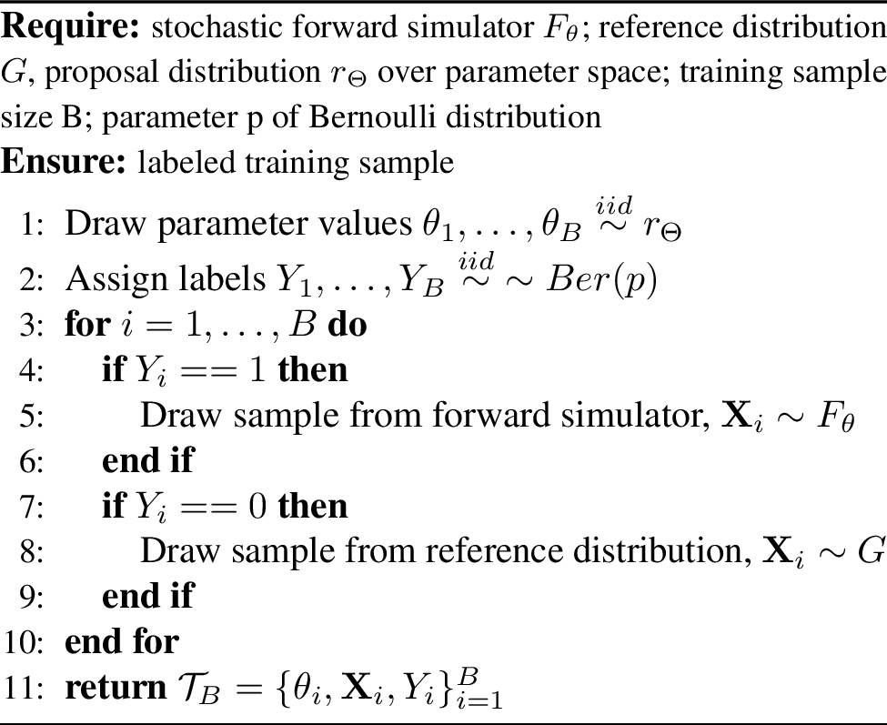
Algorithm 7 provides details on how to create the training sample \({\mathcal{T}}_B\) for estimating odds ratios. Out of the total training sample size \(B\), a proportion \(p\) is generated by the stochastic forward simulator \(F_\theta\) at different parameter values \(\theta\), while the remainder is sampled from a reference distribution \(G\).
8 Algorithm for Constructing Confidence Set for \(\theta\)↩︎
Algorithm 8 summarizes the ACORE procedure for constructing confidence sets. First, we estimate parametrized odds to compute the ACORE test statistic \(\tau\)
(Eq. 4 ). Then, we compute a parametrized estimate of the critical values as a conditional distribution function of \(\tau\). Finally, we compute a confidence set for \(\theta\) by the Neyman inversion technique [18].
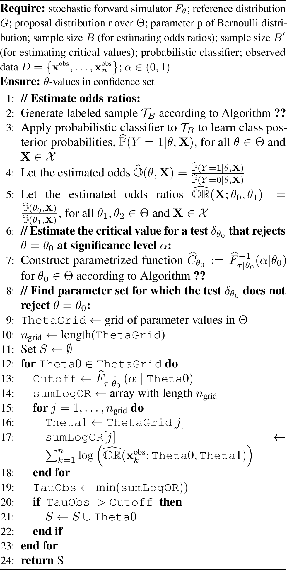
9 Proofs↩︎
Proof of Proposition [prop::consistency]. If \(\;\widehat{\mathbb{P}}(Y=1|\theta,{\mathbf{x}})=\mathbb{P}(Y=1|\theta,{\mathbf{x}})\), then \(\widehat{\mathbb{OR}}({\mathbf{x}};\theta_0,\theta_1) = \mathbb{OR}({\mathbf{x}};\theta_0,\theta_1)\). By Bayes rule and construction (Algorithm 7), \[{\mathbb{O}}({\mathbf{x}};\theta):=\frac{\mathbb{P}(Y=1|\theta,{\mathbf{x}})}{\mathbb{P}(Y=0|\theta,{\mathbf{x}})}=\frac{f({\mathbf{x}}|\theta)p}{g({\mathbf{x}})(1-p)}.\] Thus, the odds ratio at \(\theta_0,\theta_1 \in \Theta\) is given by \[\mathbb{OR}({\mathbf{x}};\theta_0,\theta_1)= \frac{f({\mathbf{x}}|\theta_0)}{f({\mathbf{x}}|\theta_1)},\] and therefore \[\begin{align} \tau(D;\Theta_0)=&\sup_{\theta_0 \in \Theta_0} \;\inf_{\theta_1 \in \Theta} \sum_{i=1}^n \left( \log \widehat{\mathbb{OR}}({\mathbf{x}}_i^{\text{obs}};\theta_0,\theta_1)\right)\\ &=\sup_{\theta_0 \in \Theta_0} \;\inf_{\theta_1 \in \Theta} \sum_{i=1}^n \log \frac{f({\mathbf{x}}_i^{\text{obs}}|\theta_0)}{f({\mathbf{x}}_i^{\text{obs}}|\theta_1)} \\ &=\sup_{\theta_0 \in \Theta_0} \;\inf_{\theta_1 \in \Theta} \log \left( \frac{{\mathcal{L}}(D;\theta_0)}{{\mathcal{L}}(D;\theta_1)}\right)\\ &=\Lambda(D;\Theta_0). \end{align}\] ◻
Proof of Theorem 1. The union bound and Assumption 1 imply that \[\sup_{\theta \in \Theta_0} \sup_{t \in \mathbb{R}}|\hat{F}_{B'}(t|\theta)- F(t|\theta)|\xrightarrow[B' \longrightarrow\infty]{\enskip \mathbb{P}\enskip} 0.\] It follows that \[\sup_{\theta \in \Theta_0} |\hat{F}^{-1}_{B'}(\alpha|\theta)- F^{-1}(\alpha|\theta)|\xrightarrow[B' \longrightarrow\infty]{\enskip \mathbb{P}\enskip} 0.\] The result follows from the fact that \[\begin{align} 0 \leq |C_{B,B'}-C_B^*|&= |\sup_{\theta \in \Theta_0} \hat{F}^{-1}_{B'}(\alpha|\theta)-\sup_{\theta \in \Theta_0} F^{-1}(\alpha|\theta)| \\ &\leq \sup_{\theta \in \Theta_0} |\hat{F}^{-1}_{B'}(\alpha|\theta)- F^{-1}(\alpha|\theta)|, \end{align}\] and thus \[|C_{B,B'}-C_B^*| \xrightarrow[B' \longrightarrow\infty]{\enskip \mathbb{P}\enskip} 0.\] ◻
Lemma 1. If \((\widehat{\mathbb{P}}(Y=1|\theta,{\mathbf{X}}))_{\theta \in \Theta} \xrightarrow[B \longrightarrow\infty]{\enskip \mathbb{P}\enskip} (\mathbb{P}(Y=1|\theta,{\mathbf{X}}))_{\theta \in \Theta}\) and \(|\Theta|<\infty\), then \[\tau({\mathcal{D}}; \Theta_0) \xrightarrow[B \longrightarrow\infty]{\enskip \mathbb{P}\enskip} \sup_{\theta_0 \in \Theta_0}\inf_{\theta_1 \in \Theta} \sum_{i=1}^n \log \left( \mathbb{OR}({\mathbf{X}}_i^{\text{obs}};\theta_0,\theta_1)\right)\]
Proof. For every \(\theta_0,\theta_1 \in \Theta\), it follows directly from the properties of convergence in probability that \[\begin{align} \sum_{i=1}^n \log & \left( \widehat{\mathbb{OR}}({\mathbf{X}}_i^{\text{obs}};\theta_0,\theta_1)\right) \\ & \xrightarrow[B \longrightarrow\infty]{\enskip \mathbb{P}\enskip} \sum_{i=1}^n \log \left( \mathbb{OR}({\mathbf{X}}_i^{\text{obs}};\theta_0,\theta_1)\right) \end{align}\]
The conclusion of the lemma follows from the continuous mapping theorem. ◻
Proof of Theorem 2. Lemma 1 implies that \(\tau_B({\mathcal{D}}; \Theta_0)\) converges in distribution to \(\sup_{\theta_0 \in \Theta_0}\inf_{\theta_1 \in \Theta}\sum_{i=1}^n \log \left( \mathbb{OR}({\mathbf{X}}_i^{\text{obs}};\theta_0,\theta_1)\right)\). Now, from Slutsky’s theorem, \[\begin{align} \tau_B&({\mathcal{D}}; \Theta_0)-\widehat{C}_B \\ &\xrightarrow[B \longrightarrow\infty]{\enskip Dist \enskip}\sup_{\theta_0 \in \Theta_0}\inf_{\theta_1 \in \Theta} \sum_{i=1}^n \log \left( \mathbb{OR}({\mathbf{X}}_i^{\text{obs}};\theta_0,\theta_1)\right)-C^*. \end{align}\] It follows that \[\begin{align} &\mathbb{P}\left(\widehat{\phi}_{B,\widehat{C}_B}(\mathcal{D})=1|\theta \right)= \mathbb{P}\left(\tau_B({\mathcal{D}}; \Theta_0)-\widehat{C}_B\leq 0|\theta \right) \\ &\xrightarrow[B \longrightarrow\infty]{} \mathbb{P}\Big(\sup_{\theta_0 \in \Theta_0}\inf_{\theta_1 \in \Theta} \sum_{i=1}^n \log \left( \mathbb{OR}({\mathbf{X}}_i^{\text{obs}};\theta_0,\theta_1)\right)\\ & -C^* \leq 0|\theta \Big)\\ &=\mathbb{P}\left(\phi_{C^*}(\mathcal{D})=1|\theta\right), \end{align}\] where the last equality follows from Proposition [prop::consistency]. ◻
10 Toy Examples↩︎
This section provides details on the toy examples of Section 4. We use the sklearn ecosystem [55] implementation of the following probabilistic classifiers:
multi-layer perceptron (MLP) with default parameters, but no \(L^2\) regularization (\(\alpha =0\));
quadratic discriminant analysis (QDA) with default parameters;
nearest neighbors (NN) classifier, with number of neighbors equal to the rounded square root of the number of data points available (as per [56]).
Table 2 reports the observed coverage for the settings of Tables 1 and ¿tbl:tab:cross95ent95poisson?. Critical values or \(C\) are estimated with quantile gradient boosted trees (\(100\) trees with maximum depth equal to \(3\)), a training sample size \(B^{'}=5000\), observed data \(D\) of sample size \(n=10\), nominal coverage of \(90\%\), and averaging over \(100\) repetitions. The table shows that we for all cases achieve results in line with the nominal confidence level.5
| \(B\) | Classifier | Poisson Example | GMM Example |
| Coverage | Coverage | ||
| 100 | MLP | 0.91 | 0.87 |
| NN | 0.91 | 0.91 | |
| QDA | 0.90 | 0.88 | |
| 500 | MLP | 0.91 | 0.91 |
| NN | 0.93 | 0.95 | |
| QDA | 0.94 | 0.92 | |
| 1000 | MLP | 0.91 | 0.92 |
| NN | 0.89 | 0.88 | |
| QDA | 0.91 | 0.93 |
Our goodness-of-fit procedure shown in Figure 5 uses a set \(\mathcal{T}^{''}_{B^{''}}\) with size \(B^{''}=250\) (as defined in Section 3.3); Figure 9 shows the goodness-of-fit plot for the Gaussian mixture model example, where the coverage is estimated via logistic regression and the critical values are estimated via quantile gradient boosted trees. For the Poisson example a training sample size of \(B'=500\) seems to be enough to achieve correct coverage, whereas the Gaussian mixture model example requires \(B'=1000\).
Next we compare our goodness-of-fit diagnostic with diagnostics obtained via standard Monte Carlo sampling. Figure 10 shows the MC coverage as a function of \(\theta\) for
the Poisson example (left) and the Gaussian mixture model example (right). In both cases 100 MC samples are drawn at 100 parameter values chosen uniformly. The empirical ACORE coverage is computed over the MC samples at each chosen \(\theta\). This MC procedure is expensive: it uses a total of \(10,000\) simulations, which is \(40\) times the number used in our goodness-of-fit procedure. The
observed coverage of the Poisson example (Figure 10, left) indicates that \(B'=500\) is sufficient to achieve the nominal coverage of \(90\%\). For the Gaussian mixture model example (Figure 10, right), we detect undercoverage for very small values of \(\theta\). This discrepancy
is due to the fact that, at \(\theta=0\), the mixture collapses into a single Gaussian, structurally different from the GMM at any other \(\theta > 0\) and closer to the \(\mathcal{N}(0, 5^2)\) reference distribution.
Our goodness-of-fit procedure is able to identify that the actual coverage is far from the nominal coverage at small values of \(\theta\), when the training sample size \(B'\) for estimating \(C\) is too small. More specifically, Figure 9 shows a noticeable tilt in the prediction bands for \(B'=100\) and \(500\). However, as \(B'\) increases, the estimation of critical values becomes more precise and the estimated confidence intervals pass our goodness-of-fit diagnostic at, for example, \(B'=1000\). Future studies will provide a more detailed account on how such boundary effects depend on the method for estimating the coverage.


Figure 10: Observed ACORE coverage across the parameter space for the Poisson example (left) and the Gaussian mixture model example (right). The coverage is computed with Monte Carlo samples of size \(100\), each sampled at a \(\theta\) chosen uniformly over the parameter space. Odds ratios are computed with a QDA classifier for the Poisson example, and an MLP classifier for the GMM example
(as in Figures 5 and 9). We observe undercoverage at small \(\theta\) for the GMM (right) due to the mixture collapsing into
a single Gaussian as \(\theta \to 0\)..
11 Signal Detection in High Energy Physics↩︎
Here we consider the signal detection example in Section 5 We describe the details of the construction of ACORE confidence sets which used the strategy in Section 5 to choose ACORE components and parameters. For learning the odds ratio, we compared the following classifiers:
logistic regression,
quadratic discimininant analysis (QDA) classifier,
nearest neighbor classifier,
gradient boosted trees using \(\{100, 500, 1000\}\) trees with maximum depth \(\{3,5,10\}\),
Gaussian process classifiers6 with radial basis functions kernels with variance \(\{1,.5,.1\}\),
feed-forward deep neural networks, with \({2,...,6}\) deep layers, number of neurons between \(2^{\{4,...,10\}}\) and either ReLu or hyperbolic tangent activations.
For estimating the critical values, we considered the following quantile regression algorithms:
gradient boosted trees using \(\{100, 250, 500\}\) trees with maximum depth \(\{3,5,10\}\),
random forest quantile regression with \(\{100, 250, 500\}\) trees,
deep quantile regression with \(\{2,3\}\) deep layers, \(2^{\{4,..,6\}}\) neurons and ReLu activations (using the
PyTorchimplementation [57]).
All computations were performed on 8-Core Intel Xeon CPUs X5680 at 3.33GHz.
Figure 11 illustrates the two steps in identifying the four components of ACORE. We first use a validation set of \(5,000\) simulations to determine which
probabilistic classifier and training sample size \(B\) minimize the cross entropy loss. Figure 11 (left) shows the cross entropy loss of the best four classifiers as function
of \(B\). The minimum is achieved by a 5-layer deep neural network (DNN) at \(B=100,000\) with a cross entropy loss of \(58.509\times 10^{-2}\), closely
followed by QDA with \(58.512\times 10^{-2}\) at \(B=50,000\). Given how similar the loss values are, we select both classifiers to follow-up on. In Figure 11 (right), the “estimated correct coverage” represents the proportion of the parameter space that passes our diagnostic procedure. The lowest \(B'\) with correct coverage is
achieved by the five-layer DNN classifier (for estimating odds ratios) at \(B'=25,000\) with critical values estimated via a two-layer deep quantile regression algorithm. None of the quantile regression algorithms pass
a diagnostic test with a nominal coverage of \(90\%\) at the one standard deviation level when using the QDA classifier. We therefore do not use QDA in Section 5.
Based on the analysis above, we choose the following ACORE components: (i) a five-layer DNN for learning odds ratios, (ii) \(B=100,000\), (iii) a two-layer deep quantile regression for estimating critical
values, and (iv) \(B'=25,000\). Figure 6 shows the confidence sets computed with this choice.


Figure 11: Using the strategy in Section 5 to choose ACORE components for the signal detection example. Left: The cross entropy loss of the best four classifiers, shown as a
function of \(B\). In order of increasing loss: 5-layer DNN ([512, 256, 64, 32, 32] neurons, ReLu activations), QDA classifier, 3-layer DNN ([64, 32, 32] neurons, ReLu activations) and gradient boosted trees (\(1000\) trees with maximum depth 5). Because the first two classifiers (the 5-layer DNN and QDA) achieve a very similar minimum loss, we consider both classifiers in the follow-up step. Right: Proportion of the \((\nu, b)\) parameter space where the best two classifiers pass our goodness-of-fit procedure with a nominal coverage of \(90\%\). Both the mean value curves and the \(\pm\) one standard deviation prediction bands are computed via logistic regression. Critical values are estimated via a two-layer deep quantile regression ([64,64] neurons, ReLu activations), which passed the diagnostic at the
lowest sample size (\(B'=25,000\), with the 5-layers DNN). Based on the results, we choose the 5-layer DNN with \(B'=25,000\)..
12 Cross Entropy Loss Analysis↩︎
In this work, we use the cross entropy loss to measure the accuracy of the probabilistic predictions of the classifier. That is, we calibrate the estimated odds function \(g(\theta,{\mathbf{x}}) := \widehat{\mathbb{P}}(Y=1 |
\theta, {\mathbf{x}})/\widehat{\mathbb{P}}(Y=0 | \theta, {\mathbf{x}})\) as follows: Consider a sample point \(\{\theta,{\mathbf{x}},y\}\) generated according to Algorithm 7. Let \(p\) be a \(Ber(y)\) distribution, and \(q\) be a \(Ber\left(\widehat{\mathbb{P}}(Y=1 | \theta,
{\mathbf{x}})\right)=Ber\left(\frac{g(\theta,{\mathbf{x}})}{1+g(\theta,{\mathbf{x}})}\right)\) distribution. The cross entropy between \(p\) and \(q\) is given by \[\begin{align} L_{CE}(g; \{\theta,{\mathbf{x}},y\}) &= - y \log\left(\frac{g(\theta,{\mathbf{x}})}{1+g(\theta,{\mathbf{x}})}\right) \\
&\quad \quad \quad - (1-y) \log\left(\frac{1}{1+g(\theta,{\mathbf{x}})}\right) \\
&= - y \log \left(g(\theta,{\mathbf{x}}) \right) + \log \left(1+g(\theta,{\mathbf{x}}) \right).
\end{align}\] For every \({\mathbf{x}}\) and \(\theta\), the expected cross entropy \(\mathbb{E}[L_{CE}(g; \{\theta,{\mathbf{x}},Y\})]\) is minimized
by \(g(\theta,{\mathbf{x}})=\mathbb{O}(\theta,{\mathbf{x}})\). Thus we can measure the performance of an estimator \(g\) of the odds by the risk \[R_{CE}(g)=\mathbb{E}[L_{CE}(g; \{\theta,{\mathbf{X}},Y\})] .\] The cross entropy loss is not the only loss function that is minimized by the true odds function, but it is usually easy to compute in practice. It is also well
known that minimizing the cross entropy loss between the estimated distribution \(q\) and the true distribution \(p\) during training is equivalent to minimizing the Kullback-Leibler (KL)
divergence between the two distributions, as \[KL(p || q) = H(p, q) - H(p),\] where \(H(p,q)\) is the cross entropy and \(H(p)\) is the entropy of the true
distribution. By Gibbs’ inequality [58], we have that \(KL(p|| q) \geq 0\); hence
the entropy \(H(p)\) of the true distribution lower bounds the cross entropy with the minimum achieved when \(p=q\). Hence, we can connect the cross entropy loss to the ACORE
statistic.
If the probabilistic classifier in ACORE achieves the minimum of the cross entropy loss, then the constructed ACORE statistic 4 is equal to the likelihood ratio statistic 3 .
Proof of Prop [prop::cross95ent95lrt]. The proof follows from Proposition [prop::consistency] and the expected cross entropy loss is minimized if and only if \(\widehat{\mathbb{O}}(\theta,{\mathbf{x}})=\mathbb{O}(\theta,{\mathbf{x}})\). ◻
In addition, we show that the convergence of the class posterior implies the convergence of the cross entropy to the entropy of the true distribution. This supports our decision to use the cross entropy loss when selecting the probabilistic classifier and sample size \(B\).
Lemma 2. If for every \(\theta \in \Theta\) \[q := \widehat{\mathbb{P}}(Y=1|\theta,{\mathbf{X}}) \xrightarrow[B \longrightarrow\infty]{\enskip \mathbb{P}\enskip} p:=\mathbb{P}(Y=1|\theta,{\mathbf{X}}),\] then \(H(p, q) \xrightarrow[B \longrightarrow\infty]{\enskip \mathbb{P}\enskip} H(p).\)
Proof of Lemma 2. We can rewrite the cross entropy \(H(p, q)\) and entropy \(H(p)\) as \[\begin{align} H(p, q) & = - \sum_{y \in \{0,1\} } \int_{\mathcal{X} \times \Theta} p \log\left(q \right) {\rm d}\mathbb{P}({\mathbf{x}},\theta), \\ H(p) & = - \sum_{y \in \{0,1\} } \int_{\mathcal{X} \times \Theta} p \log\left(p \right) {\rm d}\mathbb{P}({\mathbf{x}},\theta). \end{align}\] In addition, for any \(({\mathbf{X}}, \theta)\), it also holds that \(\left|q\right| \leq 1\). The lemma follows by combining the dominated convergence theorem with the continuous mapping theorem for the logarithm. ◻
13 Comparison with Monte Carlo Synthetic Likelihood-Based Methods↩︎
In this section we compare the performance of ACORE with Monte-Carlo (MC) synthetic likelihood-based methods, more specifically Gaussian process (GP) interpolation [29]. The latter method first simulates multiple sample points for a few different values of \(\theta\). For each fixed \(\theta\), one fits a Gaussian synthetic likelihood function. The GP likelihood model is then used to smoothly interpolate across the parameter space by fitting a mean function \(m(\theta)\) and
a covariance function \(\Sigma(\theta)\). As a note, [14] point out that such MC
methods are less efficient than methods that estimate the likelihood ratio directly because of the need to first estimate the entire likelihood.
For our comparison, we use the two toy examples described in Section 4 and Table 1. To allocate \(B\) sample points for the GP interpolation, we use the following strategy: For \(q \in \{5, 10 ,25\}\), first choose \(\theta_1, ..., \theta_q\) on an evenly spaced grid across the parameter space. Then, generate \(N=B/q\) sample points \(\mathbf{X}_1, ... ,\mathbf{X}_N\) at each location \(\theta\).
Table ¿tbl:tab:comparison95with95MC? summarizes the results. Unlike Table ¿tbl:tab:cross95ent95poisson?, we do not report the cross-entropy loss because GP interpolation is not a classification algorithm; instead we
report the mean squared error in estimating the likelihood ratio across the parameter space. Our results show that when the simulated data at each \(\theta\) are approximately Gaussian, as in the Poisson example, MC-based
GP interpolation provides a better approximation of the likelihood ratio due to its parametric assumptions. However, when the parametric assumptions are not valid, as in the GMM example, MC-based GP fails to approximate the likelihood ratio regardless of
how large \(N\) or \(B\) are. In such settings, we do better with a fully nonparametric approach. As a note, MC-based GP uses the asymptotic \(\chi^2\)
approximation by Wilks’ theorem to determine the critical values of the confidence sets. In our experiments, using quantile regression for critical values instead (as in ACORE) led to a significant increase in power for the GP likelihood
models: from \(\approx 0.48\) to \(\approx 0.51\) for the Poisson example, and from \(\approx 0.02\) to \(\approx 0.2\) for
the GMM example.
| Poisson Example | ||||
|---|---|---|---|---|
| \(B\) | Classifier | 90 \(\%\) Mean Squared | Average | Size of |
| Error Interval | Power | Confidence Set [%] | ||
| 100 | MLP | [2.14, 989.78] | 0.27 | 72.8 \(\pm\) 16.4 |
| NN | [4.14, 4074.65] | 0.25 | 75.6 \(\pm\) 23.2 | |
| QDA | [0.41, 34.79] | 0.41 | 60.1 \(\pm\) 14.9 | |
| G.P. (5) | [0.05, 4.09] | 0.47 | 53.5 \(\pm\) 9.2 | |
| G.P. (10) | [0.06, 4.97] | 0.48 | 53.2 \(\pm\) 10.7 | |
| G.P. (25) | [0.03, 6.54] | 0.48 | 53.2 \(\pm\) 10.8 | |
| 500 | MLP | [0.86, 22.45] | 0.38 | 62.2 \(\pm\) 19.1 |
| NN | [1.95, 32.78] | 0.37 | 64.2 \(\pm\) 17.3 | |
| QDA | [0.08, 6.95] | 0.45 | 55.5 \(\pm\) 10.8 | |
| G.P. (5) | [0.01, 0.81] | 0.49 | 52.4 \(\pm\) 5.6 | |
| G.P. (10) | [0.02, 0.85] | 0.49 | 52.0 \(\pm\) 5.4 | |
| G.P. (25) | [0.01, 1.12] | 0.48 | 52.5 \(\pm\) 6.0 | |
| 1,000 | MLP | [0.81, 21.44] | 0.42 | 58.8 \(\pm\) 17.0 |
| NN | [1.77, 17.88] | 0.45 | 56.1 \(\pm\) 16.2 | |
| QDA | [0.06, 2.83] | 0.49 | 52.1 \(\pm\) 9.0 | |
| G.P. (5) | [0.01, 0.48] | 0.49 | 52.3 \(\pm\) 5.0 | |
| G.P. (10) | [0.01, 0.46] | 0.48 | 52.5 \(\pm\) 5.3 | |
| G.P. (25) | [0.01, 0.45] | 0.48 | 52.6 \(\pm\) 5.5 | |
| - | Exact | - | 0.54 | 45.0 \(\pm\) 4.9 |
| GMM Example | ||||
|---|---|---|---|---|
| \(B\) | Classifier | 90 \(\%\) Mean Squared | Average | Size of |
| Error Interval (\(\times 10^3\)) | Power | Confidence Set [%] | ||
| 100 | MLP | [0.34, 1.46] | 0.87 | 14.5 \(\pm\) 4.5 |
| NN | [1.33, 11.77] | 0.49 | 52.1 \(\pm\) 24.7 | |
| QDA | [2.88, 3.56] | 0.16 | 84.0 \(\pm\) 21.8 | |
| G.P. (5) | [3.35, 3.82] | 0.02 | 97.7 \(\pm\) 8.8 | |
| G.P. (10) | [3.34, 3.82] | 0.03 | 96.9 \(\pm\) 9.5 | |
| G.P. (25) | [3.36, 3.82] | 0.02 | 98.2 \(\pm\) 6.1 | |
| 500 | MLP | [0.44, 1.35] | 0.90 | 12.1 \(\pm\) 2.8 |
| NN | [0.99, 2.65] | 0.57 | 44.0 \(\pm\) 23.3 | |
| QDA | [3.14, 3.73] | 0.16 | 83.8 \(\pm\) 22.2 | |
| G.P. (5) | [3.39, 3.83] | 0.00 | 100.0 \(\pm\) 0.0 | |
| G.P. (10) | [3.39, 3.83] | 0.01 | 99.1 \(\pm\) 5.5 | |
| G.P. (25) | [3.38, 3.83] | 0.00 | 99.8 \(\pm\) 1.5 | |
| 1,000 | MLP | [0.53, 1.17] | 0.90 | 12.1 \(\pm\) 2.8 |
| NN | [0.57, 2.04] | 0.71 | 30.2 \(\pm\) 18.5 | |
| QDA | [3.26, 3.94] | 0.14 | 85.7 \(\pm\) 20.1 | |
| G.P. (5) | [3.39, 3.98] | 0.00 | 100.0 \(\pm\) 0.0 | |
| G.P. (10) | [3.39, 3.98] | 0.00 | 100.0 \(\pm\) 0.0 | |
| G.P. (25) | [3.39, 3.98] | 0.00 | 99.9 \(\pm\) 1.2 | |
| - | Exact | - | 0.92 | 9.5 \(\pm\) 2.0 |
14 Comparison with Calibrated Approximate Ratio of Likelihood Classifiers↩︎
In this section we compare the performance of ACORE with the calibrated approximate ratio of likelihood (CARL) estimator by [28]. CARL approximates the likelihood ratio \(\Lambda(D; \Theta_0) = \mathcal{L}(D; \theta_0)/\mathcal{L}(D; \theta_1)\) by turning the density ratio estimation into a supervised
classification problem, where a probabilistic classifier is trained to separate samples from \(F_{\theta_0}\) and \(F_{\theta_1}\). As such, CARL classifiers are “doubly parameterized” by
\(\theta_0\) and \(\theta_1\), whereas the ACORE classifier is parameterized by a single parameter \(\theta\) in the definition of the
odds of \(F_\theta\) versus \(G\).
In our study, we include three different CARL classifiers, implemented with the MADMINER neural network-based software [59], [60]: (a) a shallow perceptron with 100 neurons (equivalent to the MLP used in Section 4), (b) a 2-layer deep
network with 20 neurons per layer, and (c) a 2-layer deep network with 20 and 50 neurons in the two layers respectively.7 To allocate \(B\)
sample points for interpolation we devised two schemes: (i) a uniform sampling, and (ii) a Monte Carlo sampling over the parameter space. For (i), we uniformly sample \(B\) parameters and then generate a sample point \(\mathbf{X}\) at each parameter value. For (ii), we first select evenly spaced parameters \(\theta_{0,1}, ..., \theta_{0,q}\) and \(\theta_{1,1} ..., \theta_{1,
q}\), for the numerator and the denominator respectively. We set \(q \in \{10, 20, 30\}\), resulting in \(N=B/q\) sample points \(\mathbf{X}_1, ...,
\mathbf{X}_N\) at each \(\theta\) location. Because the \(\chi^2\) approximation by Wilks’ theorem did not yield valid confidence sets for CARL classifiers, we computed critical
values as in ACORE Algorithm 3.
Table ¿tbl:tab:comparison95with95carl? shows the results of ACORE and CARL for the synthetic data in Section 4 and Table 1.
For both the Poisson and GMM examples, CARL classifiers yield a higher mean squared error in estimating the likelihood ratio, as well as lower power and larger confidence intervals.
| Poisson Example | ||||
|---|---|---|---|---|
| \(B\) | Classifier | 90 \(\%\) Mean Squared | Average | Size of |
| Error Interval | Power | Confidence Set [%] | ||
| 200 | MLP | [3.25, 1305.45] | 0.17 | 82.7 \(\pm\) 15.0 |
| NN | [2.88, 185.47] | 0.34 | 66.9 \(\pm\) 20.7 | |
| QDA | [0.20, 25.16] | 0.45 | 55.8 \(\pm\) 13.2 | |
| MLP (MC) | [2.51, 38.10] | 0.24 | 76.1 \(\pm\) 21.3 | |
| (20,20) DNN (MC) | [2.53, 25.41] | 0.19 | 80.9 \(\pm\) 17.8 | |
| (50,20) DNN (MC) | [2.76, 26.00] | 0.19 | 81.3 \(\pm\) 17.8 | |
| MLP (U) | [2.03, 45.19] | 0.19 | 81.3 \(\pm\) 19.2 | |
| (20,20) DNN (U) | [2.95, 19.76] | 0.24 | 76.6 \(\pm\) 19.8 | |
| (50,20) DNN (U) | [2.43, 18.72] | 0.23 | 77.8 \(\pm\) 20.1 | |
| 800 | MLP | [1.69, 450.81] | 0.27 | 73.0 \(\pm\) 20.1 |
| NN | [1.47, 19.32] | 0.42 | 59.2 \(\pm\) 15.9 | |
| QDA | [0.04, 5.03] | 0.49 | 52.0 \(\pm\) 9.3 | |
| MLP (MC) | [2.38, 24.50] | 0.22 | 78.5 \(\pm\) 21.0 | |
| (20,20) DNN (MC) | [2.49, 21.49] | 0.25 | 75.3 \(\pm\) 18.8 | |
| (50,20) DNN (MC) | [2.52, 18.13] | 0.23 | 76.9 \(\pm\) 20.1 | |
| MLP (U) | [2.04, 23.24] | 0.20 | 79.9 \(\pm\) 17.4 | |
| (20,20) DNN (U) | [2.48, 17.36] | 0.22 | 77.9 \(\pm\) 17.6 | |
| (50,20) DNN (U) | [2.25, 17.87] | 0.21 | 78.9 \(\pm\) 20.0 | |
| 1,800 | MLP | [0.81, 19.11] | 0.37 | 63.7 \(\pm\) 21.1 |
| NN | [1.09, 11.27] | 0.44 | 56.9 \(\pm\) 14.3 | |
| QDA | [0.03, 1.60] | 0.50 | 51.0 \(\pm\) 6.6 | |
| MLP (MC) | [2.13, 35.39] | 0.18 | 82.4 \(\pm\) 17.7 | |
| (20,20) DNN (MC) | [2.74, 28.15] | 0.20 | 80.3 \(\pm\) 19.7 | |
| (50,20) DNN (MC) | [2.62, 28.15] | 0.18 | 81.9 \(\pm\) 19.5 | |
| MLP (U) | [2.15, 25.51] | 0.19 | 81.4 \(\pm\) 19.8 | |
| (20,20) DNN (U) | [2.34, 15.93] | 0.23 | 77.0 \(\pm\) 22.6 | |
| (50,20) DNN (U) | [2.38, 17.97] | 0.19 | 81.6 \(\pm\) 17.2 | |
| - | Exact | - | 0.54 | 45.0 \(\pm\) 4.9 |
| GMM Example | ||||
|---|---|---|---|---|
| \(B\) | Classifier | 90 \(\%\) Mean Squared | Average | Size of |
| Error Interval (\(\times 10^{3}\)) | Power | Confidence Set [%] | ||
| 200 | MLP | [0.56, 1.69] | 0.88 | 14.2 \(\pm\) 8.2 |
| NN | [1.13, 4.17] | 0.50 | 51.5 \(\pm\) 24.8 | |
| QDA | [3.05, 3.63] | 0.12 | 87.6 \(\pm\) 19.7 | |
| MLP (MC) | [3.03, 3.61] | 0.27 | 73.5 \(\pm\) 20.5 | |
| (20,20) DNN (MC) | [3.13, 3.70] | 0.25 | 75.6 \(\pm\) 20.0 | |
| (50,20) DNN (MC) | [3.16, 3.67] | 0.28 | 72.8 \(\pm\) 19.6 | |
| MLP (U) | [3.01, 3.72] | 0.30 | 70.2 \(\pm\) 21.2 | |
| (20,20) DNN (U) | [3.18, 3.87] | 0.24 | 76.3 \(\pm\) 21.5 | |
| (50,20) DNN (U) | [3.12, 3.92] | 0.27 | 73.0 \(\pm\) 21.2 | |
| 800 | MLP | [0.89, 1.59] | 0.90 | 12.1 \(\pm\) 2.5 |
| NN | [0.78, 2.31] | 0.69 | 32.0 \(\pm\) 18.9 | |
| QDA | [3.23, 3.66] | 0.14 | 86.1 \(\pm\) 20.4 | |
| MLP (MC) | [3.02, 3.58] | 0.30 | 70.8 \(\pm\) 20.4 | |
| (20,20) DNN (MC) | [3.10, 3.63] | 0.27 | 73.6 \(\pm\) 20.2 | |
| (50,20) DNN (MC) | [3.03, 3.47] | 0.30 | 70.5 \(\pm\) 18.5 | |
| MLP (U) | [3.01, 3.62] | 0.26 | 74.7 \(\pm\) 20.6 | |
| (20,20) DNN (U) | [3.12, 3.64] | 0.26 | 74.4 \(\pm\) 19.2 | |
| (50,20) DNN (U) | [3.00, 3.56] | 0.29 | 71.8 \(\pm\) 19.9 | |
| 1,800 | MLP | [0.33, 1.55] | 0.90 | 11.5 \(\pm\) 2.6 |
| NN | [0.32, 1.57] | 0.83 | 19.3 \(\pm\) 10.3 | |
| QDA | [3.29, 3.81] | 0.16 | 83.7 \(\pm\) 22.2 | |
| MLP (MC) | [2.99, 3.54] | 0.33 | 67.5 \(\pm\) 19.6 | |
| (20,20) DNN (MC) | [3.02, 3.54] | 0.31 | 69.7 \(\pm\) 19.3 | |
| (50,20) DNN (MC) | [2.95, 3.51] | 0.38 | 63.1 \(\pm\) 15.9 | |
| MLP (U) | [2.99, 3.45] | 0.33 | 67.7 \(\pm\) 17.0 | |
| (20,20) DNN (U) | [3.02, 3.56] | 0.33 | 67.3 \(\pm\) 18.0 | |
| (50,20) DNN (U) | [2.98, 3.41] | 0.38 | 63.1 \(\pm\) 15.3 | |
| - | Exact | - | 0.92 | 9.5 \(\pm\) 2.0 |
15 Runtime Analysis↩︎
In this section we provide a runtime analysis for constructing one ACORE confidence set for the two examples in Section 4 and Table ¿tbl:tab:cross95ent95poisson?. We also provide a
running time comparison with the two methods described in Sections 13 and 14. This analysis was performed on a 8-Core Intel Xeon 3.33GHz X5680 CPU.
The procedure for constructing confidence sets with ACORE is outlined in Algorithm 8. In this analysis we break the computation into 4 steps: (i) odds ratio training as described by Algorithm 7, (ii) computing the test statistic 4 for the observed data, (iii) computing the test statistic 4 in the \(B^{'}\) sample as described by Algorithm 4 and (iv) quantile regression algorithm training. Table ¿tbl:tab:running95times? summarizes our running times
results. ACORE constructs one confidence set in less than \(20\) and \(30\) seconds for Poisson and GMM examples respectively. The main computational bottleneck is step (iii),
while the computation time of step (i) increases with the sample size \(B\).
Figure 12 shows the results of comparing confidence set construction runtimes with MC GP and CARL classifiers. For both the Poisson and the GMM examples, we only consider the best performing ACORE
classifiers, and the two CARL classifiers with 20 hidden units in both layers. Results show ACORE classifiers are comparable with GP interpolation in terms of running times, while CARL classifiers tend to have significantly longer
runtimes.
| Running Times to Generate a Confidence Set (Seconds) – Poisson Example | ||||||
|---|---|---|---|---|---|---|
| \(B\) | Classifier | Odds Ratio | Odds Ratio | Calculate [eq:odds95ratio95statistic] for | Quantile Regression | Total Running |
| Training | Prediction | \(B^{'}\) Samples | Training | Time | ||
| 100 | MLP | 0.38 \(\pm\) 0.31 | 0.42 \(\pm\) 0.10 | 10.40 \(\pm\) 0.71 | 0.66 \(\pm\) 0.28 | 11.86 \(\pm\) 1.02 |
| NN | 0.03 \(\pm\) 0.01 | 0.35 \(\pm\) 0.12 | 9.83 \(\pm\) 4.99 | 0.82 \(\pm\) 0.67 | 11.02 \(\pm\) 5.73 | |
| QDA | 0.02 \(\pm\) 0.01 | 0.18 \(\pm\) 0.11 | 4.50 \(\pm\) 2.65 | 0.58 \(\pm\) 0.21 | 5.29 \(\pm\) 2.96 | |
| 500 | MLP | 1.62 \(\pm\) 0.39 | 0.46 \(\pm\) 0.04 | 11.49 \(\pm\) 0.45 | 0.68 \(\pm\) 0.09 | 14.26 \(\pm\) 0.61 |
| NN | 0.13 \(\pm\) 0.01 | 0.54 \(\pm\) 0.03 | 13.28 \(\pm\) 0.26 | 0.66 \(\pm\) 0.04 | 14.60 \(\pm\) 0.29 | |
| QDA | 0.13 \(\pm\) 0.01 | 0.16 \(\pm\) 0.01 | 4.12 \(\pm\) 0.09 | 0.65 \(\pm\) 0.06 | 5.05 \(\pm\) 0.14 | |
| 1,000 | MLP | 2.65 \(\pm\) 0.88 | 0.48 \(\pm\) 0.08 | 11.93 \(\pm\) 1.93 | 0.73 \(\pm\) 0.06 | 15.79 \(\pm\) 2.30 |
| NN | 0.24 \(\pm\) 0.04 | 0.77 \(\pm\) 0.21 | 17.90 \(\pm\) 2.82 | 0.67 \(\pm\) 0.10 | 19.59 \(\pm\) 2.83 | |
| QDA | 0.27 \(\pm\) 0.08 | 0.17 \(\pm\) 0.05 | 4.37 \(\pm\) 1.02 | 0.64 \(\pm\) 0.16 | 5.45 \(\pm\) 1.29 | |
| Running Times to Generate a Confidence Set (Seconds) – GMM Example | ||||||
|---|---|---|---|---|---|---|
| \(B\) | Classifier | Odds Ratio | Odds Ratio | Calculate [eq:odds95ratio95statistic] for | Quantile Regression | Total Running |
| Training | Prediction | \(B^{'}\) Samples | Training | Time | ||
| 100 | MLP | 5.89 \(\pm\) 1.66 | 0.45 \(\pm\) 0.18 | 10.79 \(\pm\) 2.06 | 0.60 \(\pm\) 0.21 | 17.74 \(\pm\) 3.92 |
| NN | 0.03 \(\pm\) 0.00 | 0.29 \(\pm\) 0.06 | 8.60 \(\pm\) 2.84 | 0.61 \(\pm\) 0.18 | 9.53 \(\pm\) 3.05 | |
| QDA | 0.03 \(\pm\) 0.01 | 0.14 \(\pm\) 0.04 | 3.81 \(\pm\) 1.38 | 0.52 \(\pm\) 0.14 | 4.50 \(\pm\) 1.57 | |
| 500 | MLP | 9.89 \(\pm\) 1.34 | 0.43 \(\pm\) 0.06 | 11.64 \(\pm\) 0.64 | 0.69 \(\pm\) 0.06 | 22.64 \(\pm\) 1.83 |
| NN | 0.17 \(\pm\) 0.01 | 0.52 \(\pm\) 0.04 | 13.11 \(\pm\) 0.79 | 0.63 \(\pm\) 0.07 | 14.43 \(\pm\) 0.85 | |
| QDA | 0.16 \(\pm\) 0.01 | 0.15 \(\pm\) 0.02 | 4.05 \(\pm\) 0.26 | 0.59 \(\pm\) 0.08 | 4.94 \(\pm\) 0.35 | |
| 1,000 | MLP | 13.40 \(\pm\) 2.60 | 0.47 \(\pm\) 0.09 | 11.76 \(\pm\) 0.79 | 0.68 \(\pm\) 0.11 | 26.31 \(\pm\) 3.36 |
| NN | 0.34 \(\pm\) 0.09 | 0.70 \(\pm\) 0.11 | 17.15 \(\pm\) 1.90 | 0.71 \(\pm\) 0.17 | 18.90 \(\pm\) 2.06 | |
| QDA | 0.32 \(\pm\) 0.05 | 0.17 \(\pm\) 0.05 | 4.75 \(\pm\) 1.26 | 0.62 \(\pm\) 0.07 | 5.87 \(\pm\) 1.36 | |

References↩︎
That is, \(\widehat{\phi}_{B,C_B}(\mathcal{D})=1 \iff \tau_B({\mathcal{D}}; \Theta_0) < C_B\).↩︎
That is, \(\phi_{C^*}(\mathcal{D})=1 \iff \Lambda({\mathcal{D}}; \Theta_0) < C^*\).↩︎
More specifically, an 8-core Intel Xeon 3.33GHz X5680 CPU.↩︎
In traditional settings, high power has been shown to lead to a small expected interval size under certain distributional assumptions [45], [46].↩︎
The \(95\%\) CI of a binomial distribution with probability \(p=0.9\) over \(100\) repetitions is in fact \([0.84, 0.95]\). This interval includes the observed coverages listed in Table 2.↩︎
GP classifiers were used only with sample sizes \(B\) below \(10,000\), as the matrix inversion quickly becomes computationally infeasible for larger values of \(B\).↩︎
Changing the number of neurons per layers did not seem to provide a significant difference in performance for the 2-layer deep networks. Number of epochs and learning rate were manually tuned (with a search in the range \([20, 200]\) and \(10^{\{ -6, ..., -2\}}\) respectively).↩︎