A Discriminative Gaussian Mixture Model with Sparsity
November 14, 2019
Abstract
In probabilistic classification, a discriminative model based on the softmax function has a potential limitation in that it assumes unimodality for each class in the feature space. The mixture model can address this issue, although it leads to an increase in the number of parameters. We propose a sparse classifier based on a discriminative GMM, referred to as a sparse discriminative Gaussian mixture (SDGM). In the SDGM, a GMM-based discriminative model is trained via sparse Bayesian learning. Using this sparse learning framework, we can simultaneously remove redundant Gaussian components and reduce the number of parameters used in the remaining components during learning; this learning method reduces the model complexity, thereby improving the generalization capability. Furthermore, the SDGM can be embedded into neural networks (NNs), such as convolutional NNs, and can be trained in an end-to-end manner. Experimental results demonstrated that the proposed method outperformed the existing softmax-based discriminative models.
Acknowledgments↩︎
This work was supported in part by JSPS KAKENHI Grant Number JP17K12752 and JST ACT-I Grant Number JPMJPR18UO.
Supplementary materials↩︎
1 Relationship between the discriminative Gaussian and logistic regression↩︎
We show that a fully connected layer with the softmax function, or logistic regression, can be regarded as a discriminative model based on a Gaussian distribution by utilizing transformation of the equations. Let us consider a case in which the class-conditional probability \(P(\boldsymbol{x}|c)\) is a Gaussian distribution. In this case, we can omit \(m\) from the equations ([eq:PosteriorProb])–([eq:ParameterCollapsing]).
If all classes share the same covariance matrix and the mixture weight \(\pi_{cm}\), the terms \(\pi_{cm}\) in ([ep:ComponentDiscriminativeModel]), \(x_1^2, x_1x_2, \ldots, x_1x_D, x_2^2, x_2x_3, \ldots, x_2x_D, \ldots, x_D^2\) in ([eq:NonlinearTrans]), and \(-\frac{1}{2}s_{c11}, \ldots\!, -\frac{1}{2}s_{cDD}\) in ([eq:ParameterCollapsing]) can be canceled; hence the calculation of the posterior probability \(P(c|\boldsymbol{x})\) is also simplified as \[P(c|\boldsymbol{x}) = \frac{\exp({\boldsymbol{w}_{c}}^{\rm T}\boldsymbol{\phi})}{\sum^{C}_{c=1}\exp({\boldsymbol{w}_{c}}^{\rm T}\boldsymbol{\phi})},\nonumber\] where \[\begin{align} \boldsymbol{w}_{c} &= [\log P(c) - \frac{1}{2}\sum^{D}_{i=1}\sum^{D}_{j=1}s_{cij}\mu_{ci}\mu_{cj} + \frac{D}{2}\log{2\pi} + \frac{1}{2}\log{|\boldsymbol{\Sigma}_{c}|}, \sum^{D}_{i=1}s_{ci1}\mu_{ci},\cdots\!,\sum^{D}_{i=1}s_{ciD}\mu_{ci}]^\mathrm{T},\nonumber \\ \boldsymbol{\phi} &= \left[1, \boldsymbol{x}^{\rm T} \right]^{\mathrm{T}}. \nonumber \end{align}\] This is equivalent to a fully connected layer with the softmax function, or linear logistic regression.
2 Evaluation of characteristics using synthetic data↩︎
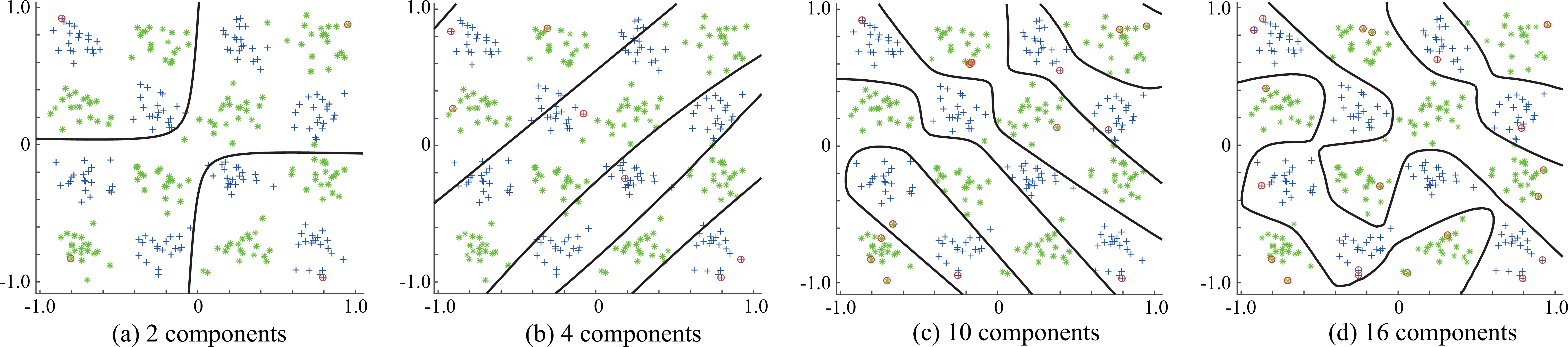
To evaluate the characteristics of the SDGM, we conducted classification experiments using synthetic data. The dataset comprises two classes. The data were sampled from a Gaussian mixture model with eight components for each class. The numbers of training data and test data were 320 and 1,600, respectively. The scatter plot of this dataset is shown in Figure 1.
In the evaluation, we calculated the error rates for the training data and the test data, the number of components after training, the number of nonzero weights after training, and the weight reduction ratio (the ratio of the number of the nonzero weights to the number of initial weights), by varying the number of initial components as \(2, 4, 8, \ldots, 20\). We repeated evaluation five times while regenerating the training and test data and calculated the average value for each evaluation criterion. We used the dual form of the SDGM in this experiment.
Figure 1 displays the changes in the learned class boundaries according to the number of initial components. When the number of components is small, such as that shown in Figure 1 (a), the decision boundary is simple; therefore, the classification performance is insufficient. However, according to the increase in the number of components, the decision boundary fits the actual class boundaries. It is noteworthy that the SDGM learns the GMM as a discriminative model instead of a generative model; an appropriate decision boundary was obtained even if the number of components for the model is less than the actual number (e.g., 1 (c)).
Figure 2 shows the evaluation results of the characteristics. Figures 2 (a), (b), (c), and (d) show the recognition error rate, number of components after training, number of nonzero weights after training, and weight reduction ratio, respectively. The horizontal axis shows the number of initial components in all the graphs.
In Figure 2 (a), the recognition error rates for the training data and test data are almost the same with the few numbers of components and decrease according to the increase in the number of initial components while it is 2 to 6. This implied that the representation capability was insufficient when the number of components was small, and that the network could not accurately separate the classes. Meanwhile, changes in the training and test error rates were both flat when the number of initial components exceeded eight, even though the test error rates were slightly higher than the training error rate. In general, the training error decreases and the test error increases when the complexity of the classifier is increased. However, the SDGM suppresses the increase in complexity using sparse Bayesian learning, thereby preventing overfitting.
In Figure 2 (b), the number of components after training corresponds to the number of initial components until the number of initial components is eight. When the number of initial components exceeds ten, the number of components after training tends to be reduced. In particular, eight components are reduced when the number of initial components is 20. The results above indicate the SDGM can reduce unnecessary components.
From the results in Figure 2 (c), we confirm that the number of nonzero weights after training increases according to the increase in the number of initial components. This implies that the complexity of the trained model depends on the number of initial components, and that the minimum number of components is not always obtained.
Meanwhile, in Figure 2 (d), the weight reduction ratio increases according to the increase in the number of initial components. This result suggests that the larger the number of initial weights, the more weights were reduced. Moreover, the weight reduction ratio is greater than 99 % in any case. The results above indicate that the SDGM can prevent overfitting by obtaining high sparsity and can reduce unnecessary components.

3 Details of initialization↩︎
In the experiments during this study, each trainable parameters for the \(m\)-th component of the \(c\)-th class were initialized as follows (\(H = 1+D(D+3)/2\), where \(D\) is the input dimension, for the original form and \(H = N\), where \(N\) is the number of the training data, for the kernelized form):
\(\boldsymbol{w}_{cm}\) (for the original form): A zero vector \(\boldsymbol{0} \in \mathbb{R}^{H}\).
\(\boldsymbol{\psi}_{cm}\) (for the kernelized form): A zero vector \(\boldsymbol{0} \in \mathbb{R}^{H}\).
\(\boldsymbol{\alpha}_{cm}\): An all-ones vector \(\boldsymbol{1} \in \mathbb{R}^{H}\).
\(\pi_{cm}\): A scalar \(\frac{1}{\sum_{c=1}^C{M_c}}\), where \(C\) is the number of classes and \(M_c\) is the number of components for the \(c\)-th class.
\(r_{ncm}\): Initialized based on the results of \(k\)-means clustering applied to the training data; \(r_{ncm} = 1\) if the \(n\)-th sample belongs to class \(c\) and is assigned to the \(m\)-th component by \(k\)-means clustering, \(r_{ncm} = 0\) otherwise.