Observing Dialogue in Therapy:
Categorizing and Forecasting Behavioral Codes
June 30, 2019
Abstract
Automatically analyzing dialogue can help understand and guide behavior in domains such as counseling, where interactions are largely mediated by conversation. In this paper, we study modeling behavioral codes used to asses a psychotherapy treatment style called Motivational Interviewing (MI), which is effective for addressing substance abuse and related problems. Specifically, we address the problem of providing real-time guidance to therapists with a dialogue observer that (1) categorizes therapist and client MI behavioral codes and, (2) forecasts codes for upcoming utterances to help guide the conversation and potentially alert the therapist. For both tasks, we define neural network models that build upon recent successes in dialogue modeling. Our experiments demonstrate that our models can outperform several baselines for both tasks. We also report the results of a careful analysis that reveals the impact of the various network design tradeoffs for modeling therapy dialogue.
1 Introduction↩︎
Conversational agents have long been studied in the context of psychotherapy, going back to chatbots such as ELIZA [1] and PARRY [2]. Research in modeling such dialogue has largely sought to simulate a participant in the conversation.
In this paper, we argue for modeling dialogue observers instead of participants, and focus on psychotherapy. An observer could help an ongoing therapy session in several ways. First, by monitoring fidelity to therapy standards, a helper could guide both veteran and novice therapists towards better patient outcomes. Second, rather than generating therapist utterances, it could suggest the type of response that is appropriate. Third, it could alert a therapist about potentially important cues from a patient. Such assistance would be especially helpful in the increasingly prevalent online or text-based counseling services.1
| Code | Count | Description | Examples |
|---|---|---|---|
| Client Behavioral Codes | |||
| 47715 | Follow/ Neutral: unrelated to changing or sustaining behavior. | “You know, I didn’t smoke for a while.” | |
| “I have smoked for forty years now.” | |||
| 5099 | Utterances about changing unhealthy behavior. | “I want to stop smoking.” | |
| 4378 | Utterances about sustaining unhealthy behavior. | “I really don’t think I smoke too much.” | |
| Therapist Behavioral Codes | |||
| 17468 | Facilitate conversation | “Mm Hmm.”, “OK.”,“Tell me more.” | |
| 15271 | Give information or feedback. | “I’m Steve.”, “Yes, alcohol is a depressant.” | |
| 6246 | Simple reflection about the client’s most recent utterance. | C: “I didn’t smoke last week” | |
| T: “Cool, you avoided smoking last week.” | |||
| 4651 | Complex reflection based on a client’s history or the broader conversation. | C: “I didn’t smoke last week.” | |
| T: “You mean things begin to change”. | |||
| 5218 | Closed question | “Did you smoke this week?” | |
| 4509 | Open question | “Tell me more about your week.” | |
| 3869 | Other MI adherent,, affirmation, advising with permission, etc. | “You’ve accomplished a difficult task.” | |
| “Is it OK if I suggested something?” | |||
| 1019 | MI non-adherent, , confrontation, advising without permission, etc. | “You hurt the baby’s health for cigarettes?” | |
| “You ask them not to drink at your house.” | |||
We ground our study in a style of therapy called Motivational Interviewing [3], [4], which is widely used for treating addiction-related problems. To help train therapists, and also to monitor therapy quality, utterances in sessions are annotated using a set of behavioral codes called Motivational Interviewing Skill Codes [5]. Table ¿tbl:tbl:misc? shows standard therapist and patient (, client) codes with examples. Recent NLP work [6]–[8], [9] inter alia has studied the problem of using MISC to assess completed sessions. Despite its usefulness, automated post hoc MISC labeling does not address the desiderata for ongoing sessions identified above; such models use information from utterances yet to be said. To provide real-time feedback to therapists, we define two complementary dialogue observers:
Categorization: Monitoring an ongoing session by predicting MISC labels for therapist and client utterances as they are made.
Forecasting: Given a dialogue history, forecasting the MISC label for the next utterance, thereby both alerting or guiding therapists.
Via these tasks, we envision a helper that offers assistance to a therapist in the form of MISC labels.
We study modeling challenges associated with these tasks related to:
representing words and utterances in therapy dialogue,
ascertaining relevant aspects of utterances and the dialogue history, and
handling label imbalance (as evidenced in Table ¿tbl:tbl:misc?).
We develop neural models that address these challenges in this domain.
Experiments show that our proposed models outperform baselines by a large margin. For the categorization task, our models even outperform previous session-informed approaches that use information from future utterances. For the more difficult forecasting task, we show that even without having access to an utterance, the dialogue history provides information about its MISC label. We also report the results of an ablation study that shows the impact of the various design choices.2. In summary, in this paper, we
define the tasks of categorizing and forecasting Motivational Interviewing Skill Codes to provide real-time assistance to therapists,
propose neural models for both tasks that outperform several baselines, and
show the impact of various modeling choices via extensive analysis.
2 Background and Motivation↩︎
Motivational Interviewing (MI) is a style of psychotherapy that seeks to resolve a client’s ambivalence towards their problems, thereby motivating behavior change. Several meta-analyses and empirical studies have shown the high efficacy and success of MI in psychotherapy [10]–[12]. However, MI skills take practice to master and require ongoing coaching and feedback to sustain [13]. Given the emphasis on using specific types of linguistic behaviors in MI (, open questions and reflections), fine-grained behavioral coding plays an important role in MI theory and training.
Motivational Interviewing Skill Codes (MISC, table ¿tbl:tbl:misc?) is a framework for coding MI sessions. It facilitates evaluating therapy sessions via utterance-level labels that are akin to dialogue acts [14], [15], and are designed to examine therapist and client behavior in a therapy session.3
As Table ¿tbl:tbl:misc? shows, client labels mark utterances as discussing changing or sustaining problematic behavior (Ct and St, respectively) or being neutral (Fn). Therapist utterances are grouped into eight labels, some of which (Res, Rec) correlate with improved outcomes, while MI non-adherent (Min) utterances are to be avoided. MISC labeling was originally done by trained annotators performing multiple passes over a session recording or a transcript. Recent NLP work speeds up this process by automatically annotating a completed MI session [6]–[8].
Instead of providing feedback to a therapist after the completion of a session, can a dialogue observer provide online feedback? While past work has shown the helpfulness of post hoc evaluations of a session, prompt feedback would be more helpful, especially for MI non-adherent responses. Such feedback opens up the possibility of the dialogue observer influencing the therapy session. It could serve as an assistant that offers suggestions to a therapist (novice or veteran) about how to respond to a client utterance. Moreover, it could help alert the therapist to potentially important cues from the client (specifically, Ct or St).
3 Task Definitions↩︎
In this section, we will formally define the two NLP tasks corresponding to the vision in §2 using the conversation in table ¿tbl:tbl:example? as a running example.
Suppose we have an ongoing MI session with utterances \(u_1, u_2,\cdots, u_n\): together, the dialogue history \(H_n\). Each utterance \(u_i\) is associated with its speaker \(s_i\), either C (client) or T (therapist). Each utterance is also associated with the MISC label \(l_i\), which is the object of study. We will refer to the last utterance \(u_n\) as the anchor.
We will define two classification tasks over a fixed dialogue history with \(n\) elements — categorization and forecasting. As the conversation progresses, the history will be updated with a sliding window. Since the therapist and client codes share no overlap, we will design separate models for the two speakers, giving us four settings in all.
| \(i\) | \(s_{i}\) | \(u_{i}\) | \(l_{i}\) |
|---|---|---|---|
| 1 | T: | Have you used drugs recently? | |
| 2 | C: | I stopped for a year, but relapsed. | |
| 3 | T: | You will suffer if you keep using. | |
| 4 | C: | Sorry, I just want to quit. | |
| \(\cdots\) | \(\cdots\) | \(\cdots\) |
Task 1: Categorization. The goal of this task is to provide real-time feedback to a therapist during an ongoing MI session. In the running example, the therapist’s confrontational response in the third utterance is not MI adherent (Min); an observer should flag it as such to bring the therapist back on track. The client’s response, however, shows an inclination to change their behavior (Ct). Alerting a therapist (especially a novice) can help guide the conversation in a direction that encourages it.
In essence, we have the following real-time classification task: Given the dialogue history \(H_n\) which includes the speaker information, predict the MISC label \(l_n\) for the last utterance \(u_n\).
The key difference from previous work in predicting MISC labels is that we are restricting the input to the real-time setting. As a result, models can only use the dialogue history to predict the label, and in particular, we can not use models such as a conditional random field or a bi-directional LSTM that need both past and future inputs.
Task 2: Forecasting. A real-time therapy observer may be thought of as an expert therapist who guides a session with suggestions to the therapist. For example, after a client discloses their recent drug use relapse, a novice therapist may respond in a confrontational manner (which is not recommended, and hence coded Min). On the other hand, a seasoned therapist may respond with a complex reflection (Rec) such as “Sounds like you really wanted to give up and you’re unhappy about the relapse.” Such an expert may also anticipate important cues from the client. The forecasting task seeks to mimic the intent of such a seasoned therapist: Given a dialogue history \(H_n\) and the next speaker’s identity \(s_{n+1}\), predict the MISC code \(l_{n+1}\) of the yet unknown next utterance \(u_{n+1}\).
The MISC forecasting task is a previously unstudied problem. We argue that forecasting the type of the next utterance, rather than selecting or generating its text as has been the focus of several recent lines of work [16]–[18], allows the human in the loop (the therapist) the freedom to creatively participate in the conversation within the parameters defined by the seasoned observer, and perhaps even rejecting suggestions. Such an observer could be especially helpful for training therapists [19]. The forecasting task is also related to recent work on detecting antisocial comments in online conversations [20] whose goal is to provide an early warning for such events.
4 Models for MISC Prediction↩︎
Modeling the two tasks defined in §3 requires addressing four questions:
How do we encode a dialogue and its utterances?
Can we discover discriminative words in each utterance?
Can we discover which of the previous utterances are relevant?
How do we handle label imbalance in our data?
Many recent advances in neural networks can be seen as plug-and-play components. To facilitate the comparative study of models, we will describe components that address the above questions. In the rest of the paper, we will use boldfaced terms to denote vectors and matrices and small caps to denote component names.
4.1 Encoding Dialogue↩︎
Since both our tasks are classification tasks over a dialogue history, our goal is to convert the sequence of utterences into a single vector that serves as input to the final classifier.
We will use a hierarchical recurrent encoder [21], [22], [23] and others to encode dialogues, specifically a hierarchical gated recurrent unit (HGRU) with an utterance and a dialogue encoder. We use a bidirectional GRU over word embeddings to encode utterances. As is standard, we represent an utterance \(u_i\) by concatenating the final forward and reverse hidden states. We will refer to this utterance vector as \(\boldsymbol{v}_i\). Also, we will use the hidden states of each word as inputs to the attention components in §4.2. We will refer to such contextual word encoding of the \(j^{th}\) word as \(\boldsymbol{v}_{ij}\). The dialogue encoder is a unidirectional GRU that operates on a concatenation of utterance vectors \(\boldsymbol{v}_i\) and a trainable vector representing the speaker \(s_i\).4 The final state of the GRU aggregates the entire dialogue history into a vector \(\boldsymbol{H}_n\).
The HGRU skeleton can be optionally augmented with the word and dialogue attention described next. All the models we will study are two-layer MLPs over the vector \(\boldsymbol{H}_n\) that use a ReLU hidden layer and a softmax layer for the outputs.
4.2 Word-level Attention↩︎
Certain words in the utterance history are important to categorize or forecast MISC labels. The identification of these words may depend on the utterances in the dialogue. For example, to identify that an utterance is a simple reflection (Res) we may need to discover that the therapist is mirroring a recent client utterance; the example in table ¿tbl:tbl:misc? illustrates this. Word attention offers a natural mechanism for discovering such patterns.
We can unify a broad collection of attention mechanisms in NLP under a single high level architecture [24]. We seek to define attention over the word encodings \(\boldsymbol{v}_{ij}\) in the history (called queries), guided by the word encodings in the anchor \(\boldsymbol{v}_{nk}\) (called keys). The output is a sequence of attention-weighted vectors, one for each word in the \(i^{th}\) utterance. The \(j^{th}\) output vector \(\boldsymbol{a}_j\) is computed as a weighted sum of the keys: \[\boldsymbol{a}_{ij} = \sum_{k} \alpha^{k}_{j} \boldsymbol{v}_{nk} \label{eq:att95sum}\tag{1}\] The weighting factor \(\alpha^k_j\) is the attention weight between the \(j^{th}\) query and the \(k^{th}\) key, computed as \[\label{eq:att95weight} \alpha^{k}_{j} = \frac{\exp\left(f_{m}(\boldsymbol{v}_{nk}, \boldsymbol{v}_{ij})\right)}{\sum_{j^{\prime}} \exp\left(f_{m}(\boldsymbol{v}_{nk}, \boldsymbol{v}_{ij^\prime})\right)}\tag{2}\] Here, \(f_m\) is a match scoring function between the corresponding words, and different choices give us different attention mechanisms.
Finally, a combining function \(f_{c}\) combines the original word encoding \(\boldsymbol{v}_{ij}\) and the above attention-weighted word vector \(\boldsymbol{a}_{ij}\) into a new vector representation \(\boldsymbol{z}_{ij}\) as the final representation of the query word encoding: \[\boldsymbol{z}_{ij}= f_{c}(\boldsymbol{v}_{ij}, \boldsymbol{a}_{ij})\]
The attention module, identified by the choice of the functions \(f_m\) and \(f_c\), converts word encodings in each utterance \(\boldsymbol{v}_{ij}\) into attended word encodings \(\boldsymbol{z}_{ij}\). To use them in the HGRU skeleton, we will encode them a second time using a BiGRU to produce attention-enhanced utterance vectors. For brevity, we will refer to these vectors as \(\boldsymbol{v}_i\) for the utterance \(u_i\). If word attention is used, these attended vectors will be treated as word encodings.
| Method | \(f_{m}\) | \(f_{c}\) |
|---|---|---|
| BiDAF | \(\bm{v}_{nk} {\bm{v}_{ij}^{T}}\) | \([\bm{v}_{ij};~\bm{a}_{ij};\) |
| \(~~\bm{v}_{ij} \odot \bm{a}_{ij};~\bm{v}_{ij}\odot \bm{a}^{\prime}]\) | ||
| GMGRU | \(\bm{w}^{e} \tanh(\bm{W}^{k}\bm{v}_{nk}\) | \([\bm{v}_{ij};\bm{a}_{ij}]\) |
| \(~~+ \bm{W}^{q}[\bm{v}_{ij}; \bm{h}_{j-1}])\) |
To complete this discussion, we need to instantiate the two functions. We use two commonly used attention mechanisms: BiDAF [25] and gated matchLSTM [26]. For simplicity, we replace the sequence encoder in the latter with a BiGRU and refer to it as GMGRU. Table ¿tbl:tbl:word95att? shows the corresponding definitions of \(f_{c}\) and \(f_{m}\). We refer the reader to the original papers for further details. In subsequent sections, we will refer to the two attended versions of the HGRU as BiDAF\(^H\) and GMGRU\(^H\).
4.3 Utterance-level Attention↩︎
While we assume that the history of utterances is available for both our tasks, not every utterance is relevant to decide a MISC label. For categorization, the relevance of an utterance to the anchor may be important. For example, a complex reflection (Rec) may depend on the relationship of the current therapist utterance to one or more of the previous client utterances. For forecasting, since we do not have an utterance to label, several previous utterances may be relevant. For example, in the conversation in Table ¿tbl:tbl:example?, both \(u_2\) and \(u_4\) may be used to forecast a complex reflection.
To model such utterance-level attention, we will employ the multi-head, multi-hop attention mechanism used in Transformer networks [27]. As before, due to space constraints, we refer the reader to the original work for details. We will use the \((\boldsymbol{Q}, \boldsymbol{K}, \boldsymbol{V})\) notation from the original paper here. These matrices represent a query, key and value respectively. The multi-head attention is defined as: \[\label{eq:multihead95attention} {\small \text{Multihead}(\boldsymbol{Q},\boldsymbol{K},\boldsymbol{V}) = [\text{head}_{1};\cdots; \text{head}_{h}]\boldsymbol{W}^{O}}\tag{3}\] \[\text{head}_{i} = \text{softmax}\left(\frac{\boldsymbol{Q}\boldsymbol{W}^{Q}_{i}\left(\boldsymbol{K}\boldsymbol{W}^{K}_{i}\right)^T}{\sqrt{d_{k}}}\right)\boldsymbol{V}\boldsymbol{W}^{V}_{i}\] The \(\boldsymbol{W}_i\)’s refer to projection matrices for the three inputs, and the final \(\boldsymbol{W}^o\) projects the concatenated heads into a single vector.
The choices of the query, key and value defines the attention mechanism. In our work, we compare two variants: anchor-based attention, and self-attention. The anchor-based attention is defined by \(Q = [\boldsymbol{v}_{n}]\) and \(K=V=[\boldsymbol{v}_{1} \cdots \boldsymbol{v}_{n}]\). Self-attention is defined by setting all three matrices to \([\boldsymbol{v}_{1} \cdots \boldsymbol{v}_{n}]\). For both settings, we use four heads and stacking them for two hops, and refer to them as \(\textcolor{dkgray}{\mathrm{\small self_{42}}}\) and \(\textcolor{dkgray}{\mathrm{\small anchor_{42}}}\).
4.4 Addressing Label Imbalance↩︎
From Table ¿tbl:tbl:misc?, we see that both client and therapist labels are imbalanced. Moreover, rarer labels are more important in both tasks. For example, it is important to identify Ct and St utterances. For therapists, it is crucial to flag MI non-adherent (Min) utterances; seasoned therapists are trained to avoid them because they correlate negatively with patient improvements. If not explicitly addressed, the frequent but less useful labels can dominate predictions.
To address this, we extend the focal loss [28] to the multiclass case. For a label \(l\) with probability produced by a model \(p_t\), the loss is defined as \[\label{eq:focal} \text{FL}(p_{t}) = -\alpha_{t} {(1 -p_{t})}^{\gamma} \log(p_{t})\tag{4}\] In addition to using a label-specific balance weight \(\alpha_t\), the loss also includes a modulating factor \({(1-p_{t})}^{\gamma}\) to dynamically downweight well-classified examples with \(p_{t}\gg0.5\). Here, the \(\alpha_t\)’s and the \(\gamma\) are hyperparameters. We use FL as the default loss function for all our models.
5 Experiments↩︎
The original psychotherapy sessions were collected for both clinical trials and Motivational Interviewing dissemination studies including hospital settings [29], outpatient clinics [30], college alcohol interventions [31]–[34]. All sessions were annotated with the Motivational Interviewing Skills Codes (MISC) [35]. We use the train/test split of [6], [36] to give 243 training MI sessions and 110 testing sessions. We used 24 training sessions for development. As mentioned in §2, all our experiments are based on the MISC codes grouped by [7].
5.1 Preprocessing and Model Setup↩︎
An MI session contains about 500 utterances on average. We use a sliding window of size \(N=8\) utterances with padding for the initial ones. We assume that we always know the identity of the speaker for all utterances. Based on this, we split the sliding windows into a client and therapist windows to train separate models. We tokenized and lower-cased utterances using spaCy [37]. To embed words, we concatenated 300-dimensional Glove embeddings [38] with ELMo vectors [39]. The appendix details the model setup and hyperparameter choices.
5.2 Results↩︎
Best Models. Our goal is to discover the best client and therapist models for the two tasks. We identified the following best configurations using \(\text{F}_{1}\) score on the development set:
Categorization: For client, the best model does not need any word or utterance attention. For the therapist, it uses GMGRU\(^H\) for word attention and anchor\(_{42}\) for utterance attention. We refer to these models as \(\mathcal{C}_C\) and \(\mathcal{C}_T\) respectively
Forecasting: For both client and therapist, the best model uses no word attention, and uses self\(_{42}\) utterance attention. We refer to these models as \(\mathcal{F}_C\) and \(\mathcal{F}_T\) respectively.
Here, we show the performance of these models against various baselines. The appendix gives label-wise precision, recall and \(\text{F}_{1}\) scores.
Results on Categorization. Tables ¿tbl:tbl:main95rst95c95categorizing? and ¿tbl:tbl:main95rst95t95categorizing? show the performance of the \(\mathcal{C}_C\) and \(\mathcal{C}_T\) models and the baselines. For both therapist and client categorization, we compare the best models against the same set of baselines. The majority baseline illustrates the severity of the label imbalance problem. [7], \(\text{BiGRU}_{\text{generic}}\), [36] and [6] are the previous published baselines. The best results of previous published baselines are underlined. The last row \(\Delta\) in each table lists the changes of our best model from them. \(\text{BiGRU}_{\text{ELMo}}\), \(\text{CONCAT}^{C}\), \(\text{GMGRU}^{H}\) and \(\text{BiDAF}^{H}\) are new baselines we define below.
3pt
| Method | macro | |||
|---|---|---|---|---|
| Majority | 30.6 | 91.7 | 0.0 | 0.0 |
| [7] | 50.0 | 87.9 | 32.8 | 29.3 |
| \(\text{BiGRU}_{\text{generic}}\) | 50.2 | 87.0 | 35.2 | 28.4 |
| \(\text{BiGRU}_{\text{ELMo}}\) | 52.9 | 87.6 | 39.2 | 32.0 |
| [36] | 44.0 | 91.0 | 20.0 | 21.0 |
| [6] | 48.3 | 89.0 | 29.0 | 27.0 |
| \(\text{CONCAT}^{C}\) | 51.8 | 86.5 | 38.8 | 30.2 |
| \(\text{GMGRU}^{H}\) | 52.6 | 89.5 | 37.1 | 31.1 |
| \(\text{BiDAF}^{H}\) | 50.4 | 87.6 | 36.5 | 27.1 |
| \(\mathcal{C}_{C}\) | 53.9 | 89.6 | 39.1 | 33.1 |
| \(\Delta=\mathcal{C}_{C} - \text{\underline{score}}\) | +3.5 | -2.1 | +3.9 | +3.8 |
| Method | macro | ||||||||
|---|---|---|---|---|---|---|---|---|---|
| Majority | 5.87 | 47.0 | 0.0 | 0.0 | 0.0 | 0.0 | 0.0 | 0.0 | 0.0 |
| [7] | 59.3 | 94.7 | 50.2 | 48.3 | 71.9 | 68.7 | 80.1 | 54.0 | 6.5 |
| \(\text{BiGRU}_{\text{generic}}\) | 60.2 | 94.5 | 50.5 | 49.3 | 72.0 | 70.7 | 80.1 | 54.0 | 10.8 |
| \(\text{BiGRU}_{\text{ELMo}}\) | 62.6 | 94.5 | 51.6 | 49.4 | 70.7 | 72.1 | 80.8 | 57.2 | 24.2 |
| [36] | - | 94.0 | 49.0 | 45.0 | 74.0 | 72.0 | 81.0 | - | - |
| [6] | - | 94.0 | 48.0 | 39.0 | 69.0 | 68.0 | 77.0 | - | - |
| \(\text{CONCAT}^{C}\) | 61.0 | 94.5 | 54.6 | 34.3 | 73.3 | 73.6 | 81.4 | 54.6 | 22.0 |
| \(\text{GMGRU}^{H}\) | 64.9 | 94.9 | 56.0 | 54.4 | 75.5 | 75.7 | 83.0 | 58.2 | 21.8 |
| \(\text{BiDAF}^{H}\) | 63.8 | 94.7 | 55.9 | 49.7 | 75.4 | 73.8 | 80.7 | 56.2 | 24.0 |
| \(\mathcal{C}_{T}\) | 65.4 | 95.0 | 55.7 | 54.9 | 74.2 | 74.8 | 82.6 | 56.6 | 29.7 |
| \(\Delta=\mathcal{C}_{T} - \text{\underline{score}}\) | +5.2 | +0.3 | +3.9 | +3.8 | +0.2 | +2.8 | +1.6 | +2.6 | +18.9 |
The first set of baselines (above the line) do not encode dialogue history and use only the current utterance encoded with a BiGRU. The work of [7] falls in this category, and uses a 100-dimensional domain-specific embedding with weighted cross-entropy loss. Previously, it was the best model in this class. We also re-implemented this model to use either ELMo or Glove vectors with focal loss.5
The second set of baselines (below the line) are models that use dialogue context. Both [36] and [6] use well-studied linguistic features and then tagging the current utterance with both past and future utterance with CRF and MEMM, respectively. To study the usefulness of the hierarchical encoder, we implemented a model that uses a bidirectional GRU over a long sequence of flattened utterance. We refer to this as \(\text{CONCAT}^{C}\). This model is representative of the work of [9], but was reimplemented to take advantage of ELMo.
For categorizing client codes, \(\text{BiGRU}_{\text{ELMo}}\) is a simple but robust baseline model. It outperforms the previous best no-context model by more than 2 points on macro \(\text{F}_{1}\). Using the dialogue history, the more sophisticated model \(\mathcal{C}_{C}\) further gets 1 point improvement. Especially important is its improvement on the infrequent, yet crucial labels Ct and St. It shows a drop in the \(\text{F}_{1}\) on the Fn label, which is essentially considered to be an unimportant, background class from the point of view of assessing patient progress. For therapist codes, as the highlighted numbers in Table ¿tbl:tbl:main95rst95t95categorizing? show, only incorporating GMGRU-based word-level attention, \(\text{GMGRU}^{H}\) has already outperformed many baselines, our proposed model \(\mathcal{F}_{T}\) which uses both GMGRU-based word-level attention and anchor-based multi-head multihop sentence-level attention can further achieve the best overall performance. Also, note that our models outperform approaches that take advantage of future utterances.
For both client and therapist codes, concatenating dialogue history with \(\text{CONCAT}^{C}\) always performs worse than the hierarchical method and even the simpler \(\text{BiGRU}_{\text{ELMo}}\).
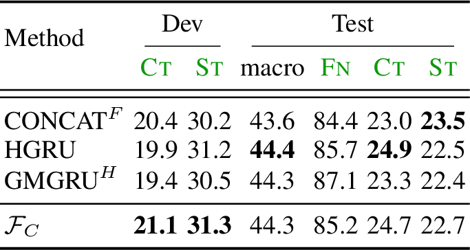
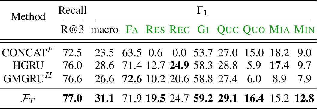
Results on Forecasting. Since the forecasting task is new, there are no published baselines to compare against. Our baseline systems essentially differ in their representation of dialogue history. The model \(\text{CONCAT}^{F}\) uses the same architecture as the model \(\text{CONCAT}^{C}\) from the categorizing task. We also show comparisons to the simple HGRU model and the GMGRU\(^H\) model that uses a gated matchGRU for word attention.6
Tables ¿tbl:tbl:main95rst95forecast? (a,b) show our forecasting results for client and therapist respectively. For client codes, we also report the Ct and St performance on the development set because of their importance. For the therapist codes, we also report the recall@3 to show the performance of a suggestion system that displayed three labels instead of one. The results show that even without an utterance, the dialogue history conveys signal about the next MISC label. Indeed, the performance for some labels is even better than some categorization baseline systems. Surprisingly, word attention (\(\text{GMGRU}^{H}\)) in Table ¿tbl:tbl:main95rst95forecast? did not help in forecasting setting, and a model with the self\(_{42}\) utterance attention is sufficient. For the therapist labels, if we always predicted the three most frequent labels (Fa, Gi, and Res), the recall@3 is only 67.7, suggesting that our models are informative if used in this suggestion-mode.
6 Analysis and Ablations↩︎
This section reports error analysis and an ablation study of our models on the development set. The appendix shows a comparison of pretrained domain-specific ELMo/glove with generic ones and the impact of the focal loss compared to simple or weighted cross-entropy.
6.1 Label Confusion and Error Breakdown↩︎
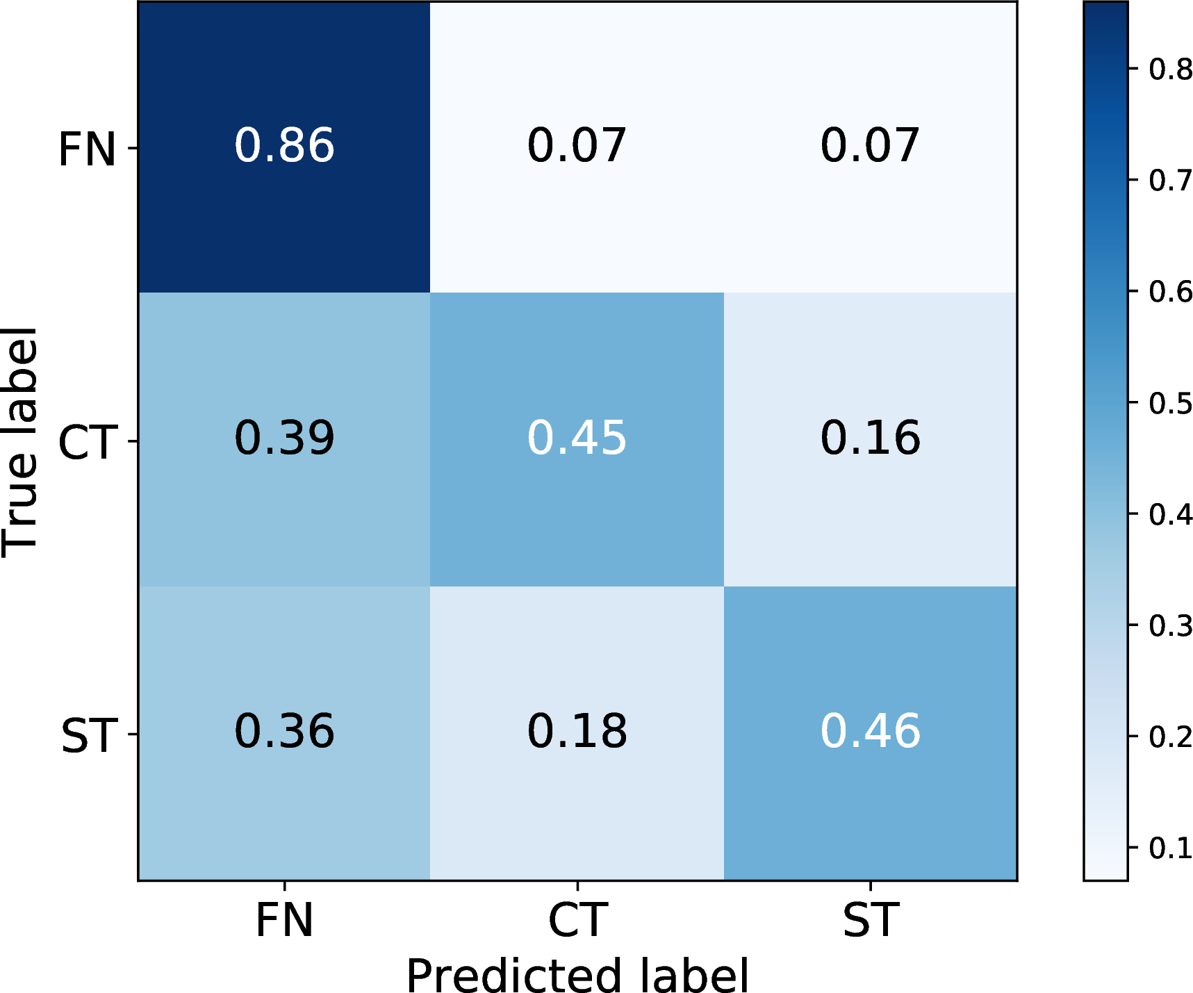
Figure 1 shows the confusion matrix for the client categorization task. The confusion between Fn and Ct/St is largely caused by label imbalance. There are 414 Ct examples that are predicted as St and 391 examples vice versa. To further understand their confusion, we selected 100 of each for manual analysis. We found four broad categories of confusion, shown in Table ¿tbl:tbl:c95client95errors?.
4pt
ll & Client Examples (Gold MISC)
&
&
&
& I mean I could try it ()
& Not a negative consequence for me ()
& I want to get every single second and minute out of it()
& It is a good thing ()
& Painful ()
& What if it does n’t work I mean what if I can’t do it ()
& But I can stop whenever I want()
The first category requires more complex reasoning than just surface form matching. For example, the phrase indicates that the client is very confident about changing behavior; the phrase indicates, in this context, that the client drinks or smokes after work. We also found that the another frequent source of error is incomplete information. In a face-to-face therapy session, people may use concise and effient verbal communication, with guestures and other body language conveying information without explaining details about, for example, coreference. With only textual context, it is difficult to infer the missing information. The third category of errors is introduced when speech is transcribed into text. The last category is about ambivalent speech. Discovering the real attitude towards behavior change behind such utterances could be difficult, even for an expert therapist.
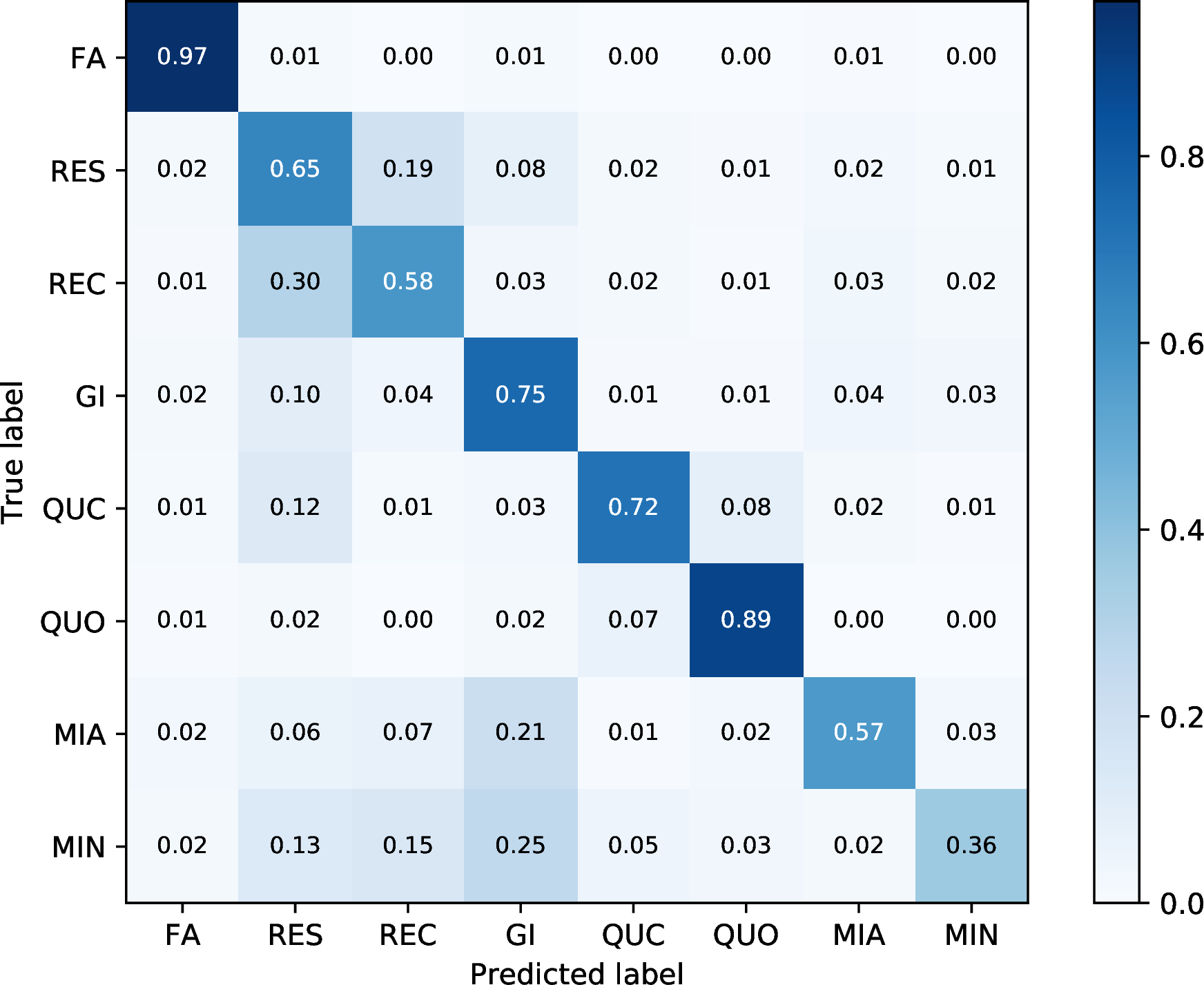
Figures 1 and 2 show the label confusion matrices for the best categorization models. We will examine confusions that are not caused purely by a label being frequent. We observe a common confusion between the two reflection labels, Rec and Res. Compared to the confusion matrix from [7], we see that our models show much-decreased confusion here. There are two reason for this confusion persisting. First, the reflections may require a much longer information horizon. We found that by increasing the window size to 16, the overall reflection results improved. Second, we need to capture richer meaning beyond surface word overlap for Res. We found that complex reflections usually add meaning or emphasis to previous client statements using devices such as analogies, metaphors, or similes rather than simply restating them. Closed questions (Quc) and simple reflections (Res) are known to be a confusing set of labels. For example, an utterance like may be both. Giving information (Gi) is easily confused with many labels because they relate to providing information to clients, but with different attitudes. The MI adherent (Mia) and non-adherent (Min) labels may also provide information, but with supportive or critical attitude that may be difficult to disentangle, given the limited number of examples.
6.2 How Context and Attention Help?↩︎
We evaluated various ablations of our best models to see how changing various design choices changes performance. We focused on the context window size and impact of different word level and sentence level attention mechanisms. Tables ¿tbl:tbl:rst95cxt95client? and ¿tbl:tbl:rst95cxt95therapist? summarize our results.
History Size. Increasing the history window size generally helps. The biggest improvements are for categorizing therapist codes (Table ¿tbl:tbl:rst95cxt95therapist?), especially for the Res and Rec. However, increasing the window size beyond 8 does not help to categorize client codes (Table ¿tbl:tbl:rst95cxt95client?) or forecasting (in appendix).
Word-level Attention. Only the model \(\mathcal{C}_{T}\) uses word-level attention. As shown in Table ¿tbl:tbl:rst95cxt95therapist?, when we remove the word-level attention from it, the overall performance drops by 3.4 points, while performances of Res and Rec drop by 3.3 and 5 points respectively. Changing the attention to BiDAF decreases performance by about 2 points (still higher than the model without attention).
Sentence-level Attention. Removing sentence attention from the best models that have it decreases performance for the models \(\mathcal{C}_T\) and \(\mathcal{F}_T\) (in appendix). It makes little impact on the \(\mathcal{F}_C\), however. Table ¿tbl:tbl:rst95cxt95client? shows that neither attention helps categorizing clients codes.
2pt
| Ablation | Options | macro | |||
|---|---|---|---|---|---|
| history window size | 0 | 51.6 | 87.6 | 39.2 | 32.0 |
| 4 | 52.6 | 88.5 | 37.8 | 31.5 | |
| \(8^{*}\) | 53.9 | 89.6 | 39.1 | 33.1 | |
| 16 | 52.0 | 89.6 | 39.1 | 33.1 | |
| word attention | + GMGRU | 52.6 | 89.5 | 37.1 | 31.1 |
| + BiDAF | 50.4 | 87.6 | 36.5 | 27.1 | |
| sentence attention | + | 53.9 | 89.2 | 39.1 | 33.2 |
| + | 53.0 | 88.2 | 38.9 | 32.0 |
3pt
| Ablation | Options | macro | |||
|---|---|---|---|---|---|
| history window size | 0 | 62.6 | 51.6 | 49.4 | 24.2 |
| 4 | 64.4 | 54.3 | 53.2 | 23.7 | |
| \(8^{*}\) | 65.4 | 55.7 | 54.9 | 29.7 | |
| 16 | 65.6 | 55.4 | 56.7 | 26.7 | |
| word attention | - GMGRU | 62.0 | 51.9 | 51.7 | 16.0 |
| \(\setminus\) BiDAF | 63.5 | 54.2 | 51.3 | 22.6 | |
| sentence attention | - | 64.9 | 56.0 | 54.4 | 21.8 |
| \(\setminus\) | 63.4 | 55.5 | 48.2 | 21.1 |
6.3 Can We Suggest Empathetic Responses?↩︎
Our forecasting models are trained on regular MI sessions, according to the label distribution on Table ¿tbl:tbl:misc?, there are both MI adherent or non-adherent data. Hence, our models are trained to show how the therapist usually respond to a given statement.
To show whether our model can mimic good MI policies, we selected 35 MI sessions from our test set which were rated 5 or higher on a 7-point scale empathy or spirit. On these sessions, we still achieve a recall@3 of 76.9, suggesting that we can learn good MI policies by training on all therapy sessions. These results suggest that our models can help train new therapists who may be uncertain about how to respond to a client.
7 Conclusion↩︎
We addressed the question of providing real-time assistance to therapists and proposed the tasks of categorizing and forecasting MISC labels for an ongoing therapy session. By developing a modular family of neural networks for these tasks, we show that our models outperform several baselines by a large margin. Extensive analysis shows that our model can decrease the label confusion compared to previous work, especially for reflections and rare labels, but also highlights directions for future work.
Acknowledgments↩︎
The authors wish to thank the anonymous reviewers and members of the Utah NLP group for their valuable feedback. This research was supported by an NSF Cyberlearning grant (#1822877) and a GPU gift from NVIDIA Corporation.
8 Appendix↩︎
8.0.0.1 Different Clustering Strategies for MISC
| Code | Count | Description | Examples |
|---|---|---|---|
| 3869 | Group of MI Adherent codes : Affirm(); Reframe(); Emphasize Control(); Support(); Filler(); Advise with permission(); Structure(); Raise concern with permission() | “You’ve accomplished a difficult task.” () | |
| “It’s your decision whether you quit or not” () | |||
| “That must have been difficult.” () | |||
| “Nice weather today!” () | |||
| “Is it OK if I suggested something?” () | |||
| “Let’s go to the next topic” () | |||
| “Frankly, it worries me.” () | |||
| 1019 | Group of MI Non-adherent codes: Confront(); Direct(); Advise without permission(); Warn(); Raise concern without permission() | “You hurt the baby’s health for cigarettes?” () | |
| “You need to xxx.” () | |||
| “You ask them not to drink at your house.” () | |||
| “You will die if you don’t stop smoking.” () | |||
| “You may use it again with your friends.” () |
The original MISC description of [5] included 28 labels (9 client, 19 therapist). Due to data scarcity and label confusion, some labels were merged into a coarser set. [36] retain 6 original labels Fa, Gi, Quc, Quo, Rec, Res, and merge remaining 13 rare labels into a single COU label, they merge all 9 client codes into a single CLI label. Instead, [6] merge only 8 of rare labels into a OTHER label and they cluster client codes according to the valence of changing, sustaining or being neutral on the addictive behavior[35]. Then [7] combine and improve above two clustering strategies by splitting the all 13 rare labels according to whether the code represents MI-adherent(Mia) and MI-nonadherent (Min) We show more details about the original labels in Mia and Min in Table ¿tbl:tbl:misc95mia95min?
8.0.0.2 Model Setup
We use 300-dimensional Glove embeddings pre-trained on 840B tokens from Common Crawl [38]. We do not update the embedding during training. Tokens not covered by Glove are using a randomly initialized UNK embedding. We also use character-level deep contextualized embedding ELMo 5.5B model by concatenating the corresponding ELMo word encoding after the word embedding vector. For speaker information, we randomly initialize them with 8 dimensional vectors and update them during training. We used a dropout rate of 0.3 for the embedding layers.
We trained all models using Adam [41] with learning rate chosen by cross validation between \([1e^{-4}, 5*1e^{-4}]\), gradient norms clipping from at \([1.0, 5.0]\), and minibatch sizes of 32 or 64. We use the same hidden size for both utterance encoder, dialogue encoder and other attention memory hidden size; it has been selected from \(\{64, 128, 256, 512\}\). We set a smaller dropout 0.2 for the final two fully connected layers. All the models are trained for 100 epochs with early-stoping based on macro \(\text{F}_{1}\) over development results.
8.0.0.3 Detailed Results of Our Main Models
In the main text, we only show the \(\text{F}_{1}\) score of each our proposed models. We summarize the performance of our best models for both categorzing and forecasting MISC codes in Table ¿tbl:tbl:main95rst? with precision, recall and \(F_{1}\) for each codes.
3pt
| Label | Categorizing | Forecasting | ||||
| P | R | \(\text{F}_{1}\) | P | R | \(\text{F}_{1}\) | |
| 92.5 | 86.8 | 89.6 | 90.8 | 80.3 | 85.2 | |
| 34.8 | 44.7 | 39.1 | 18.9 | 28.6 | 22.7 | |
| 28.2 | 39.9 | 33.1 | 19.5 | 33.7 | 24.7 | |
| 95.1 | 94.7 | 94.9 | 70.7 | 73.2 | 71.9 | |
| 50.3 | 61.3 | 55.2 | 20.1 | 18.8 | 19.5 | |
| 52.8 | 55.5 | 54.1 | 19.2 | 34.7 | 24.7 | |
| 74.6 | 75.1 | 74.8 | 52.8 | 67.5 | 59.2 | |
| 80.6 | 70.4 | 75.1 | 36.2 | 24.3 | 29.1 | |
| 85.3 | 81.2 | 83.2 | 27.0 | 11.8 | 16.4 | |
| 61.8 | 52.4 | 56.7 | 27.0 | 10.6 | 15.2 | |
| 27.7 | 28.5 | 28.1 | 17.2 | 10.2 | 12.8 | |
8.0.0.4 Domain Specific Glove and ELMo
We use the general psychotherapy corpus with 6.5M words (Alexander Street Press) to train the domain specific word embeddings \(\boldsymbol{Glove}_{psyc}\) with 50, 100, 300 dimension. Also, we trained ELMo with 1 highway connection and 256-dimensional output size to get \(\boldsymbol{ELMo}_{psyc}\). We found that ELMo 5.5B performs better than ELMo psyc in our experiments, and general Glove-300 is better than the \(\boldsymbol{Glove}_{psyc}\). Hence for main results of our models, we use \(\boldsymbol{ELMo}_{generic}\) by default. Please see more details in Table ¿tbl:tbl:rst95elmo?
| Model | Embedding | macro | macro | |||||||||||
|---|---|---|---|---|---|---|---|---|---|---|---|---|---|---|
| \(\mathcal{C}\) | \(\text{ELMo}\) | 53.9 | 89.6 | 39.1 | 33.1 | 65.4 | 95.0 | 55.7 | 54.9 | 74.2 | 74.8 | 82.6 | 56.6 | 29.7 |
| \(\text{ELMo}_{\text{psyc}}\) | 46.9 | 88.9 | 27.5 | 24.3 | 64.2 | 94.9 | 53.3 | 53.3 | 75.8 | 74.8 | 82.2 | 56.1 | 23.5 | |
| \(\text{Glove}\) | 50.6 | 89.9 | 33.4 | 28.6 | 62.2 | 94.6 | 53.7 | 54.2 | 70.3 | 70.0 | 79.1 | 54.7 | 20.9 | |
| \(\text{Glove}^{\text{pysc}}\) | 47.4 | 88.4 | 23.9 | 30.0 | 63.4 | 94.9 | 54.7 | 52.8 | 75.2 | 71.4 | 80.8 | 53.6 | 23.5 | |
| \(\mathcal{F}\) | \(\text{ELMo}\) | 44.3 | 85.2 | 24.7 | 22.7 | 31.1 | 71.9 | 19.5 | 24.7 | 59.2 | 28.3 | 17.7 | 15.9 | 9.0 |
| \(\text{ELMo}_{\text{psyc}}\) | 43.8 | 84.0 | 22.4 | 25.0 | 29.1 | 73.5 | 15.5 | 24.3 | 59.1 | 29.1 | 9.5 | 12.1 | 10.1 | |
| \(\text{Glove}\) | 42.7 | 83.9 | 21.0 | 23.1 | 30.0 | 72.8 | 20.8 | 23.7 | 58.2 | 26.2 | 14.5 | 14.5 | 9.6 | |
| \(\text{Glove}^{\text{pysc}}\) | 43.6 | 81.9 | 23.3 | 25.7 | 30.8 | 72.1 | 19.7 | 24.4 | 57.3 | 28.9 | 13.7 | 17.8 | 23.5 |
8.0.0.5 Full Results for Ablation on Forecasting Tasks
| Ablation | Options | R@3 | ||||||||||
|---|---|---|---|---|---|---|---|---|---|---|---|---|
| history size | 1 | 17.2 | 15.1 | 66.4 | 59.4 | 12.6 | 9.0 | 44.6 | 16.3 | 14.8 | 11.9 | 4.1 |
| 4 | 16.8 | 22.6 | 75.3 | 71.4 | 15.6 | 21.1 | 57.1 | 29.3 | 11.0 | 11.2 | 14.4 | |
| \(8^{*}\) | 24.7 | 22.7 | 77.0 | 72.8 | 20.8 | 23.1 | 58.1 | 28.3 | 17.7 | 15.9 | 9.0 | |
| 16 | 23.9 | 20.7 | 76.5 | 71.2 | 13.7 | 24.1 | 58.5 | 25.9 | 9.7 | 16.2 | 12.7 | |
| word attention | GMGRU | 14.0 | 23.2 | 75.7 | 71.7 | 14.2 | 23.0 | 57.5 | 26.5 | 8.0 | 15.4 | 11.6 |
| \(\text{GMGRU}_{4h}\) | 19.1 | 22.9 | 76.3 | 71.3 | 12.1 | 23.3 | 58.1 | 24.5 | 12.6 | 11.7 | 14.0 | |
| sentence attention | \(-\) | 24.9 | 22.5 | 76.0 | 71.4 | 12.7 | 24.9 | 58.3 | 28.8 | 5.9 | 17.4 | 9.7 |
| \(\setminus\) | 22.9 | 22.9 | 76.2 | 72.2 | 15.5 | 24.6 | 59.5 | 27.1 | 7.7 | 16.3 | 8.3 | |
| \(+\) GMGRU \(\setminus\) | 6.8 | 23.4 | 76.9 | 70.8 | 8.0 | 24.5 | 58.3 | 24.6 | 10.6 | 14.9 | 12.1 |
In addition to the ablation table in the main paper for categorizing tasks, we reported more ablation details on forecasting task in Table ¿tbl:tbl:rst95cxt95anticipate?. Word-level attention shows no help for both client and therapist codes. While sentence-level attention helps more on therapist codes than on client codes. Multi-head self attention alsoachieves better performance than anchor-based attention in forecasting tasks.
8.0.0.6 Label Imbalance
We always use the same \(\alpha\) for all weighted focal loss. Besides considering the label frequency, we also consider the performance gap between previous reported \(\text{F}_{1}\). We choose to balance weights \(\alpha\) as {1.0,1.0,0.25} for Ct,St and Fn respectively, and {0.5, 1.0, 1.0, 1.0, 0.75, 0.75,1.0,1.0} for Fa, Res, Rec, Gi, Quc, Quo, Mia, Min. As shown in Table ¿tbl:tbl:loss?, we report our ablation studies on cross-entropy loss, weighted cross-entropy loss, and focal loss. Besides the fixed weights, focal loss offers flexible hyperparameters to weight examples in different tasks. Experiments shows that except for the model \(\mathcal{C}^{T}\), focal loss outperforms cross-entropy loss and weighted cross entropy.
3pt
| Loss | Client | Therapist | ||||||
| \(\text{F}_{1}\) | \(\text{F}_{1}\) | |||||||
| \(\mathcal{C}^{{\text{ce}}}\) | 47.0 | 28.4 | 22.0 | 60.9 | 54.3 | 53.8 | 53.7 | 4.8 |
| \(\mathcal{C}^{\text{wce}}\) | 53.5 | 39.2 | 32.0 | 65.4 | 55.7 | 54.9 | 56.6 | 29.7 |
| \(\mathcal{C}^{\text{fl}}\) | 53.9 | 39.1 | 33.1 | 65.4 | 55.7 | 54.9 | 56.6 | 29.7 |
| \(\mathcal{F}^{{\text{ce}}}\) | 42.1 | 17.7 | 18.5 | 26.8 | 3.3 | 20.8 | 16.3 | 8.3 |
| \(\mathcal{F}^{\text{wce}}\) | 43.1 | 20.6 | 23.3 | 30.7 | 17.9 | 25.0 | 17.7 | 10.9 |
| \(\mathcal{F}^{\text{fl}}\) | 44.2 | 24.7 | 22.7 | 31.1 | 19.5 | 24.7 | 15.2 | 12.8 |
References↩︎
For example, Crisis Text Line (https://www.crisistextline.org), 7 Cups (https://www.7cups.com), etc.↩︎
The code is available online at https://github.com/utahnlp/therapist-observer.↩︎
The original MISC description of [5] included 28 labels (9 client, 19 therapist). Due to data scarcity and label confusion, various strategies are proposed to merge the labels into a coarser set. We adopt the grouping proposed by [7]; the appendix gives more details.↩︎
For the dialogue encoder, we use a unidirectional GRU because the dialogue is incomplete. For words, since the utterances are completed, we can use a BiGRU.↩︎
Other related work in no context exists [8], [40], but they either do not outperform [7] or use different data.↩︎
The forecasting task bears similarity to the next utterance selection task in dialogue state tracking work [18]. In preliminary experiments, we found that the Dual-Encoder approach used for that task consistently underperformed the other baselines described here.↩︎