1 Introduction↩︎

A prominent algorithm for applications in machine learning and statistics, such as matrix learning, recommender systems, clustering, etc., is the Conditional Gradient Method (aka Frank–Wolfe Method). Its success is based on a low per-iteration complexity in several applications. For example, in low rank approximation (e.g.matrix completion), the main computational cost per iteration is the minimization of a linear function over a nuclear norm (trace norm or Schatten 1-norm) constraint, which can be solved efficiently by approximating the singular vector associated with the largest singular value of the gradient that defines the linear function. In contrast, related proximal minimization algorithms require a full singular value decomposition, which is significantly more expensive.

In this paper, we generalize the Conditional Gradient Method to non-smooth non-convex optimization problems and unify the convergence analysis for several algorithms. The classical convergence analysis relies on the Descent Lemma, in the case the objective \(f\) has Lipschitz continuous gradient. The Descent Lemma states that \[\abs{f(x) - f(\bar x) - \scal{\nabla f(\bar x)}{x-\bar x}} \leq \frac{L}{2} \vnorm[2]{x-\bar x}^2 \quad \text{for all}\;x,\bar x\,.\] This inequality can also be interpreted as a measure for the linearization error of \(f\) around \(\bar x\), i.e., the approximation quality of \(f\) by a linear function. We emphasize the fact that such a measure for the approximation quality of \(f\), rather than smoothness, is key for the convergence of the algorithm. We generalize the linear approximation to any \(f_{\bar x}\) that obeys a certain approximation quality \[\abs{f(x) - f_{\bar x}(x)} \leq \omega(\vnorm{x-\bar x})\,,\] measured by a growth function \(\map{\omega}{\R_+}{\R_+}\) that controls the approximation error. Note that this inequality does not imply smoothness, even in the special case \(\omega(t) = \frac{L}{2}t^2\). If \(f=g+h\) with a smooth function \(h\) and a non-smooth function \(g\), we can define \(f_{\bar x}(x) = g(x) + h(\bar x) + \scal{\nabla h(\bar x)}{x-\bar x}\) and observe that the approximation error is only due to the linearization of the smooth part \(h\) of the objective, while \(f_{\bar x}\) is non-smooth. There are many other situations of interest. We choose the properties of the growth function \(\omega\) such that \(f_{\bar x}\) mimics a first order oracle of \(f\). The freedom to choose the model function depending on the problem structure at hand makes our approach a flexible and efficient way to solve structured non-smooth non-convex minimization problems.

In this model function framework, our generalized Conditional Gradient update step at \(x_{{k}}\) reads \[\begin{align} y_{{k}}\in&\;\argmin_{x\in C} f_{x_{{k}}}(x) \\ x_{{k+1}}=&\;\gamma_{{k}}y_{{k}}+ (1-\gamma_{{k}}) x_{{k}}\,, \end{align}\] where \(\gamma_{{k}}\in[0,1]\) and \(C\) is a compact and convex constraint set. For \(f_{x_{{k}}}\) being the linearization of \(f\) around \(x_{{k}}\), this is exactly the Conditional Gradient Method.

As for all methods, the efficiency depends on the cost to evaluate the oracle, which in our case is the minimization of \(f_{x_{{k}}}\) over \(C\) and, for proximal minimization problems, the cost to solve subproblems of type \[\min_{x\in \R^N} f_{x_{{k}}}(x) + \frac{1}{2\tau}\vnorm{x-x_{{k}}}^2\,,\] for some step size \(\tau>0\). The generalization achieved in this paper increases the modelling flexibility for practical applications by making them accessible with another (possibly much cheaper) oracle, or by combining the oracles to a hybrid Proximal–Conditional Gradient method. In particular, we show the favorable performance of our algorithm for a sparse non-linear robust regression problem and demonstrate the flexibility of the algorithm on several applications in matrix factorization.

2 Contributions and Related Work↩︎

The idea of model functions to unify and generalize algorithms has been used before in bundle methods [1], [2], where only a lower bound on the approximation error with the model function is used, which is a different setup. In [3], [4], the same class of model functions is considered as in our paper. In [4], a Bregman proximal minimization framework is developed and convergence to a stationary point with an Armijo-like line search strategy is proved under weak assumptions on the Bregman distances. Their work can be seen as the proximal analogue to our framework. Recently, the model function framework has been extended to stochastic optimization [5], [6].

Both, [4] and our work, present an implementable algorithm of the model function framework, which is motivated by the abstract consideration of (pure) sequential model minimization in [3]. The goal of [3] is to devise a measure for proximity to a stationary point, which can be used as a stopping criterion in non-smooth optimization. However, their convergence result depends on assumptions that are not automatically satisfied in practice. In [4], model functions are complemented with additional structure (the Bregman proximity term) and an Armijo-like line search strategy. Once the model functions are selected, convergence of subsequences to a stationary point is guaranteed. We substitute the Bregman proximity by minimization of model functions over a compact set, and also obtain convergence of subsequences to a stationary point without additional assumptions.

A special case of our framework yields the Conditional Gradient Method (aka Frank–Wolfe method [7]) with Armijo line search. Convergence has been analyzed in [8] for smooth constrained optimization and in [9] for smooth stochastic problems. While, in convex optimization, convergence of the method is fairly well understood [10]–[16], little is known in the non-smooth non-convex setting. To the best of our knowledge, our work is the first to generalize the Conditional Gradient minimization strategy to constrained non-smooth non-convex optimization with provable convergence (of subsequences) to a stationary point. In this way, we contribute to the increase in modelling flexibility for problems in machine learning, computer vision, and statistics. In particular, we explore this flexibility in an example from non-linear robust regression and several formulations from matrix factorization.

As specific instances of our algorithmic framework, we obtain new algorithms. For example, we consider non-linear composite problems of type \(\min_{x\in C} g(F(x))\) where \(F\) is sufficiently smooth and \(g\) is convex. Our iterative model function minimization over a convex constraint set yields an algorithm of Gauss-Newton type [17]. Alternative strategies that use a proximal minimization strategy, which leads to Levenberg–Marquardt algorithm [18], [19] in a certain special case, is explored, for example, in [3], [4], [20]. The problems that can be modelled in this form is immense [20]. Using specific approximations of the objective by model functions, we also propose a hybrid Proximal–Conditional Gradient minimization scheme that combines the advantages of both worlds. In the convex setting, such a hybrid method was used in [21]. However, their analysis was tailored to exactly this hybrid algorithm, whereas we obtain it from the model function framework for free and in the non-convex setting.

3 Sequential Model Minimization with Line Search↩︎

We consider optimization problems of the form \[\label{eq:objective} \min_{x\in C}\, f(x)\tag{1}\] with the following properties:

As motivated in the introduction, the proposed algorithm is based on iteratively minimizing model functions of the objective in 1 over the constraint set \(C\). These model functions obey a certain approximation quality with respect to the objective function, which we measure in general using an (error) growth function:

The standard example of a growth function is \(\omega(t)=L\cdot t^r\) with \(L>0\) and \(r>1\). However, we may easily generate more examples using the concept of \(\psi\)-uniform continuity as in [4], which generalizes Lipschitz and Hölder continuity. Note that \(\omega(t) = o(t)\) if and only if \(\omega\) is a growth function.

In this paper, we consider model functions that satisfy the following assumption.

For examples of model functions, we refer to Section 4. The Model Assumption [ass:model-assumption] preserves up to the first order information of the objective function in the following sense (see Lemma [lem:differentials]) \[\label{eq:FW-oracle} f_{\bar x}(\bar x)= f(\bar x) \quad\text{and}\quad \rpartial f(\bar x) = \partial f_{\bar x}(\bar x) \,,\tag{2}\] where \(\rpartial f\) denotes the Fréchet subdifferential [22] of \(f\) and \(\partial f\) the (convex) subdifferential, which coincides with the Fréchet subdifferential for convex functions [22]. The is defined at a point \(\bar x\), at which \(f\) is finite, as \(v\in\rpartial f(\bar x)\) if and only if \(f(x) \geq f(\bar x) + \scal{v}{x-\bar x} + o(\vnorm{x-\bar x})\), and \(\rpartial f(\bar x)=\emptyset\) for \(\bar x\not\in\dom f\).
Minimizing model functions from Assumption [ass:model-assumption] provides a generic way to define algorithms with a first order oracle (possibly non-smooth). We seek to find a \(\bar x\) of 1 , characterized by \[0 \in \rpartial f(\bar x)\,.\] In Algorithm [alg:modelFW], the proposed algorithm is defined.

Key for measuring the progress of the algorithm is the , which we define as \[\label{eq:def-model-improvement} \Delta(x,y) := f_{x}(x) - f_{x}(y) \quad \text{for all}\;x,y\in \R^N\,.\tag{3}\] Moreover, we show that it is a natural measure of stationarity. In order to obtain a “stable” algorithm, in the sense that objective values are non-increasing, the choice of \(y_{{k}}\) satisfying [eq:FW-step] is arbitrary. However, the proof that all limit points of the sequence generated by Algorithm [alg:modelFW] are stationary points requires an additional assumption. We must assert that the error in solving the model subproblem vanishes for \({k}\) tending towards infinity.

The practical realization of the Armijo condition in [eq:armijo], requires an algorithmic procedure. We propose the backtracking line search outlined in Algorithm [alg:armijo] as a subroutine for [eq:armijo].

3.1 Analysis of the Algorithm↩︎

In the following sections, we discuss Algorithm [alg:modelFW].

3.1.1 Finite Termination of the Line Search Procedure↩︎

We show that Algorithm [alg:modelFW] is well-defined, i.e., Algorithm [alg:armijo] terminates after a finite number of iterations. We verify that \(y_{{k}}-x_{{k}}\) is a , i.e., all sufficiently small choices of \(\gamma_{{k}}\) satisfy [eq:armijo]. Therefore, reducing \(\gamma_{{k}}\) according to the rule in Algorithm [alg:armijo], it eventually enters a neighborhood of \(0\) after finitely many steps.

The proof is in Section 7.1.

3.1.2 Finite Termination of the Algorithm↩︎

In case, the algorithm terminates after a finite number of iterations, i.e., [eq:FW-step] cannot be satisfied for any \(y_{{k}}\), we have already found a stationary point.

The proof is in Section 7.2.
Proposition [prop:Delta-stationarity] identifies the model improvement \(\Delta(x_{{k}},y_{{k}})\) as a suitable measure for stationarity. For smooth functions, this is an obvious fact, as the following example shows.

3.1.3 Asymptotic Analysis↩︎

In this section, we prove that all limit points of the sequence generated by Algorithm [alg:modelFW] are stationary points and that at least one such subsequence exists, which is stated in the following main convergence theorem.

The proof is in Section 7.3.

4 Examples of Model Functions↩︎

As the assumption of model functions (Assumption [ass:model-assumption]) is the same as in [4], the same examples may be incorporated here. However, we consider minimization of model functions over the constraint set \(C\) instead of (Bregman) proximal minimization. In order to make this work self contained, we mention their models (and some new ones) and discuss the algorithmic difference. For presentation, we focus on the case of maximal model improvement. Let \(\Gamma_0\) denote the class of proper lsc convex functions and \(\mathscr C^{1,\psi}(C)\) be the class of smooth functions with \(\psi\)-uniformly continuous gradient relative to \(C\), i.e., \(f\in \mathscr C^{1,\psi}\) if and only if \[\vnorm{\nabla f(x) - \nabla f(y)} \leq \psi(\vnorm{x-y})\quad \text{for all}\; x,y\in C\,,\] for some continuous function \(\map{\psi}{\R_+}{\R_+}\) with \(\psi(0)=0\). The Generalized Descent Lemma in [4] shows that such a function obeys \[\label{eq:gen-descent-lemma} \abs{f(x) - f(\bar x) - \scal{\nabla f(\bar x)}{x-\bar x}}\leq \omega(\vnorm{x-\bar x}) \quad \text{for all}\;x,\bar x\in C\,,\tag{4}\] with a growth function \(\omega(t):=\int_0^1 \frac{\phi(st)}{s}\, \mathit{d}s\) and \(\map{\phi}{\R_+}{\R_+}\) given by \(\phi(s) = s\psi(s)\). The most important example is \(\psi(s)=cs^\alpha\) for some \(c>0\), which is Hölder continuity for \(\alpha\in(0,1]\) and Lipschitz continuity for \(\alpha=1\). It results in \(\omega(t) = \frac{c}{1+\alpha} t^{1+\alpha}\). Since the optimization problem in 1 is constrained to a compact set, local Lipschitz or Hölder continuity automatically become global (possibly with a different constant).

Note that in general the following examples account for non-smooth non-convex optimization problems.

5 Applications↩︎

5.1 Sparse Robust Non-linear Regression↩︎

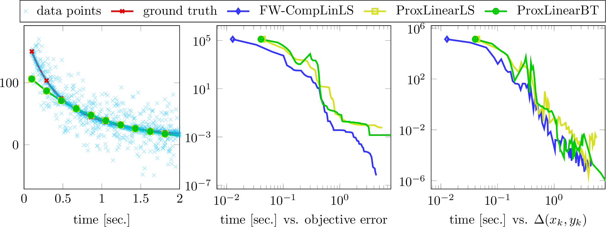
We consider a simple non-smooth non-convex sparse robust regression problem [24] of the form \[\min_{(a,b)\in C} \sum_{i=1}^M \vnorm[1]{F_i(a,b) - y_i} + \mu \vnorm[1]{a}\,, \quad F_i(a,b):= \sum_{j=1}^P a_j \exp(-b_j x_i) \,,\] similar to [4], where the data \((x_i,y_i)\in \R^2\), \(i=1,\ldots,M\), is a sequence of covariate-observation pairs and \(C = [0,\overline{a}]^P \times [0,\overline{b}]^P\) for some \(\overline{a},\overline{b}>0\) and \(P\in \N\). We assume that \(y_i = F_i(a,b) + n_i\) where \(n_i\) are iid errors drawn from a Laplacian distribution, which motivates the usage of the \(\ell_1\)-norm data fidelity term. Moreover, we assume that a large percentage of coefficients \(a_j\) are zero, which is the reason for penalizing also the \(\ell_1\)-norm of the parameter vector \(a\in \R^P\). By “symmetry” of \(F_i\), the number of zero coordinates matters rather than the actual support.

We compare several algorithms with provable convergence of subsequences to a stationary point for solving the problem. The objective function falls into the class of problems of Example [ex:prox-linear], for example, since \(F\) has bounded Hessian on \(C\), hence, its gradient is Lipschitz continuous on \(C\). All algorithms are based on that choice of model functions. We write the linearization of the inner functions around \(u_{{k}}=(a_{{k}},b_{{k}})\) as follows: For all \(i=1,\ldots,M\), \[F_i(a,b) - y_i \approx \mathcal{K}_i u - y^\diamond_i\,,\quad \text{for all}\; u=(a,b)\in C\,,\] where \(\mathcal{K}_i = D\!F_i(u_{{k}})\) and \(y^\diamond_i:=y_i - F_i(u_{{k}}) + D\!F_i(u_{{k}}) u_{{k}}\). Our Algorithm [alg:modelFW], denoted FW-CompLinLS², leads to subproblems of the form \[\min_{u=(a,b)\in C} \sum_{i=1}^M \vnorm[1]{\mathcal{K}_i u - y_i^\diamond} + \mu \vnorm[1]{a} \,,\] the algorithm in [4], denoted ProxLinearLS, and [20], denoted ProxLinearBT, require to solve subproblems of the form \[\min_{u=(a,b)\in C} \sum_{i=1}^M \vnorm[1]{\mathcal{K}_i u - y_i^\diamond} + \mu \vnorm[1]{a} + \frac{1}{2\tau}\vnorm{u - u_{{k}}}^2 \,.\] We solve the inner problem using the Primal–Dual Hybrid Gradient Algorithm with preconditioning [25], which allows for step sizes that are automatically computed based on \(\mathcal{K}_i\). We use warm starting for all methods. Our algorithm FW-CompLinLS and ProxLinearLS solve the subproblem up to a certain accuracy and perform an Armijo-like line search in the direction of the approximate solution. The backtracking of ProxLinearBT is with respect to the parameter \(\tau\) and involves solving the subproblem for each trial “step size” \(\tau\) until a sufficient improvement of the objective value is observed. All methods perform line search for improving the objective value relative to the model improvement \(\Delta(x_{{k}},y_{{k}})\). For details of the parameter setting, we refer to our code, which we provide with the paper.

The data for the experiment is generated randomly with \(P=100\), \(M=1000\), \(\mu=80\), \(\overline{a}=20\), \(\overline{b}=5\), and \(80\%\) of coefficients \(a_j\) are randomly set to \(0\). Figure [fig:rob-regr] shows the data and the convergence of the objective value or the model improvement with respect to actual computation time.

5.2 Structured Matrix Factorization↩︎

Many applications in data analysis such as blind image deblurring [26], [27], clustering and principal component analysis [28], [29], source separation [30]–[32], signal processing [33], [34], or dictionary learning [35], [36] can be formulated as structured matrix factorization problems. In this section, we demonstrate the flexible applicability of our algorithm to various formulations of matrix factorization problems. Most algorithms for solving such problems depend on alternating minimization techniques [27], [32], [34], sometimes with linearization [37], [38]. Algorithms are usually based on a proximal minimization oracle. In [4], several formulations of matrix factorization are presented using Bregman proximal minimization steps. This approach has a great advantage for several constraint sets.

However, for example, proximal minimization of low rank constraints (e.g., constraints on the nuclear norm or 1-Schatten norm) require a full singular value decomposition (SVD), which can be expensive for large (or huge) scale data analysis problems [39]. In these settings, a Conditional Gradient minimization oracle is favorable. It requires to estimate the singular vector corresponding to the largest singular value only, which is computationally significantly cheaper than a full SVD. While this technique has been used frequently in (convex) low rank approximation schemes [11], it has not been explored in detail for structured matrix factorization due to the non-convexity of the problem. We discuss several formulations of matrix factorization problems with focus on such low-rank constraints. Due to the favorable properties of the generalized Conditional Gradient minimization oracle as described above, we believe that benchmarking is not required.

We highlight the flexible applicability of our framework to non-convex problems of the form \[\min_{X,Y} \frac{1}{2} \norm[F]{A - XY}^2 + g(X) \quad \st\;X\in \mathcal{X},\;Y \in \mathcal{Y}\,,\] where the goal is to represent a matrix \(A\) as a product \(XY\) with matrices \(X\in \mathcal{X}\) and \(Y\in \mathcal{Y}\), where \(\mathcal{X}\) and \(\mathcal{Y}\) are (convex and compact) constraint sets that encode some problem specific characteristics and \(g\) is a convex regularization function. We propose to use the additive composite splitting model from Example [ex:fbs-model], i.e., we set \(C= \mathcal{X}\times \mathcal{Y}\), \(h(X,Y)=\frac{1}{2} \norm[F]{A - XY}^2\) and solve the following subproblems: \[\label{eq:FW-update-MF} \min_{X,Y} g(X) + \scal{X}{(X_{{k}}Y_{{k}}-A)Y_{{k}}^\top} + \scal{Y}{X_{{k}}^\top(X_{{k}}Y_{{k}}- A)}_F\quad \st\;X\in \mathcal{X},\;Y \in \mathcal{Y}\,.\tag{6}\] Of course, the Frobenius norm in \(h\) could be replaced by any smooth function, for example, the \(\log\)-student-t distribution \(\sum_{i,j} \log(1+(A-XY)_{i,j}^2)\) for robust estimations. The linearization of \(h\) makes the minimization separable, which allows us to discuss minimization steps with respect to \(X\) and \(Y\) independently.

5.2.0.1 Examples for \(\mathcal{X}\).

In dictionary learning, \(\mathcal{X}\) describes the set of feasible atoms that may be used for reconstructing \(A\). It is common to normalize the atoms, e.g., \[\mathcal{X}_1 = \set{X \,\vert\,\forall j\colon \sum_{i} X_{i,j}^2 \leq 1\,,\;\forall j>2\colon: \sum_{i} X_{i,j}=0}\,,\] which is a classical choice for dictionary learning [36]. For column \(j=1\), the update step in 6 is the projection of the \(1\)st column (of the gradient) onto the \(\ell_2\)-unit ball, and for \(j>1\), by projecting the mean-subtracted \(j\)th column onto the \(\ell_2\)-unit ball. The choice \[\mathcal{X}_2 = \set{X \,\vert\,\forall j\colon \sum_{i} X_{i,j} = 1\,,\;\forall i,j\colon X_{i,j}\geq 0}\] enforces normalization and non-negativity, which is commonly used in non-negative matrix factorization (NMF) [30]. The update step in 6 sets column-wise a smallest coordinates to \(1\) and all others to \(0\).

In [4], a closed form update step with respect to \(\mathcal{X}_2\) is derived by a suitable choice of Bregman distance. Proximal minimization with respect to the Euclidean distance requires an algorithmic approach, though, which is also simple, as it is just a projection onto a unit simplex.

5.2.0.2 Examples for \(\mathcal{Y}\) and \(g\).

Sparsity is a favorable property for several matrix factorization problems. Conditional Gradient steps with respect to several norm constraints lead to simple updates [11], [40]. For example, for some \(r>0\), set \(\mathcal{Y}_1= \set{Y\,\vert\,\norm[1]{Y}\leq r}\) to promote sparsity of the matrix \(Y\). It can be used in dictionary learning [36] to express \(A\) with only a few atoms of \(X\), i.e., many entries of \(Y\) shall be \(0\). Analogously, convex relaxations of rank-\(r\) constraints are commonly used, which can be modelled by \(\mathcal{Y}_2 =\set{Y \,\vert\,\norm[*]{Y} \leq r}\). The nuclear norm \(\norm[*]{Y}\) of \(Y\) enforces the columns of \(A\) to be spanned by at most \(r\) different linear subspaces, which is related to clustering problems. The Conditional Gradient subproblems with respect to both constraint sets \(\mathcal{Y}_1\) and \(\mathcal{Y}_2\) are simple [11], where the second one requires the estimation of the extreme singular vector as mentioned above.

However, on top of the constraint sets, we can use \(g\not\equiv 0\), which may be used as penalty instead of a constraint, for example, penalizing the nuclear norm [41] or structured sparsity [42]. The convex subproblem that arise in this context have been studied in convex optimization [16], [43], [44]. Also note that the solution of subproblems in 6 with respect to \(Y\) can be related to finding a subgradient in the subdifferential of the convex conjugate evaluated at the current gradient [10].

5.2.0.3 Hybrid Proximal–Conditional Gradient minimization.

Finally, we discuss an alternative model function to 6 , motivated by Example [ex:prox-FW-model]. We define the model function by linearization of the objective with respect to \(Y\) and a convex quadratic approximation with respect to \(X\). This choice leads to subproblems of the following form for our Algorithm [alg:modelFW]: \[\min_{X,Y} g(X) + \scal{X}{(X_{{k}}Y_{{k}}-A)Y_{{k}}^\top} + \scal{Y}{X_{{k}}^\top(X_{{k}}Y_{{k}}- A)}_F + \frac{1}{2\tau}\vnorm[F]{Y - Y_{{k}}}^2 \quad \st\;X\in \mathcal{X},\;Y \in \mathcal{Y}\,,\] for some \(\tau>0\), leading to Conditional Gradient type problems with respect to \(X\) and proximal minimization problems with respect to \(Y\). The matrix factorization problem and the algorithm can be formulated to explore the advantages of both worlds. For example, a nuclear norm constraint with respect to \(Y\) should be handled by a Conditional Gradient step and an additional group-sparsity penalty on \(X\) can be efficiently handled by proximal minimization steps [42].

6 Conclusion↩︎

We have presented an algorithmic framework that generalizes the Conditional Gradient method from constrained convex or smooth minimization to a class of constrained non-smooth non-convex minimization problems. The algorithm is formulated with respect to sequential minimization of model functions over the constraint set, complemented with an Armijo line search procedure. Model functions are simple surrogates of the objective function that obey a certain approximation quality and capture first order information of the problem. We presented several examples of model functions, including examples for additive or non-linear composite problems, which demonstrates the gain in flexibility for solving problems in machine learning, computer vision, and statistics. The possibility to tailor model functions to the specific structure of the optimization problem at hand, allows for efficient minimization. We also devise a hybrid method that combines Conditional Gradient type update steps with proximal minimization steps, which is particularly interesting for matrix factorization problems. In a numerical experiment for robust non-linear regression, the algorithm performs favorably compared to proximal minimization based algorithms.

Acknowledgments↩︎

This work was supported by the German Research Foundation (DFG) via grants SFB755-A4 and OC 150/1-1.

7 Proofs↩︎

7.1 Proof of Proposition [prop:armijo-finite-term]↩︎

For a fixed \(k\in \N\), we abbreviate \(\gamma=\gamma_{{k}}\). Using Assumption [ass:model-assumption], we have \[f(x_{{k+1}}) - f(x_{{k}}) \leq f_{x_{{k}}}(x_{{k+1}}) - f_{x_{{k}}}(x_{{k}}) + \omega(\vnorm{x_{{k+1}}-x_{{k}}}) \,.\] From \(\vnorm{x_{{k+1}}- x_{{k}}} = \gamma\vnorm{y_{{k}}- x_{{k}}}\) and the definition of a growth function it follows that \(\omega(\vnorm{x_{k+1}-x_k})=o(\gamma)\). The convexity of the model function \(f_{x_k}\) gives us \[f_{x_{{k}}}(x_{{k+1}}) - f_{x_{{k}}}(x_{{k}}) \leq \gamma (f_{x_{{k}}}(y_{{k}}) - f_{x_{{k}}}(x_{{k}})) \,.\] Now, we argue by contradiction. Suppose that for any \(\tilde{\gamma} >0\) there exists \(\gamma\in (0,\tilde{\gamma})\) such that [eq:armijo] does not hold, which yields the following calculation \[-\gamma \rho \Delta(x_{{k}}, y_{{k}}) < f(x_{{k+1}}) - f(x_{{k}}) \leq \gamma (f_{x_{{k}}}(y_{{k}}) - f_{x_{{k}}}(x_{{k}})) + o(\gamma) = -\gamma\Delta(x_{{k}}, y_{{k}}) + o(\gamma) \,.\] Dividing the inequality by \(\gamma\), we obtain \(0< (1-\rho) \Delta(x_{{k}}, y_{{k}}) < o(\gamma)/\gamma\), which is a contradiction for sufficiently small \(\tilde{\gamma}\).

7.2 Proof of Proposition [prop:Delta-stationarity]↩︎

The result is shown by Fermat’s rule in the following lemma.

7.3 Proof of Theorem [thm:convergence]↩︎

The result is proved in three steps.

7.3.0.1 Convergence of objective values.

The monotonicity and convergence of \(\seq[{k}\in\N]{f(x_{{k}})}\) follows directly from [eq:armijo] and the boundedness of \(f\) from below.

7.3.0.2 Vanishing model improvement.

From [eq:armijo] and convergence of \(\seq[{k}\in\N]{f(x_{{k}})}\), we infer that \(\gamma_{{k}}\Delta(x_{{k}},y_{{k}})\to 0\), since \[0 \leq \rho \gamma_{{k}}\Delta(x_{{k}},y_{{k}}) \leq f(x_{{k}}) - f(x_{{k+1}}) \to 0 \,.\] We deduce boundedness of \(\seq[{k}\in\N]{\Delta(x_{{k}},y_{{k}})}\) by \[\begin{gather} 0 \leq \Delta(x_{{k}},y_{{k}}) = f_{x_{{k}}}(x_{{k}}) - f_{x_{{k}}}(y_{{k}}) \leq f(x_{{k}}) - f_{x_{{k}}}(\hat{y}_{{k}}) \\ \leq f(x_{0}) - f(\hat{y}_{{k}}) + \omega(\vnorm{\hat{y}_{{k}}- x_{{k}}}) \leq f(x_{0}) - \inf_{x\in C} f(x) + \omega(\mathop{\mathrm{diam}}(C)) < +\infty. \end{gather}\] Let \(\Delta^*\) be an arbitrary limit point of \(\seq[{k}\in\N]{\Delta(x_{{k}},y_{{k}})}\), that is \(\Delta(x_{{k}},y_{{k}})\to\Delta^*\) as \(k\overset{K}{\to} \infty\) for some \(K\subset \N\), where \({k}\overset{K}{\to}\infty\) abbreviates \({k}\to\infty\) with \({k}\in K\).

Suppose \(\Delta^*>0\). Then \(\gamma_{{k}}\to 0\) as \({k}\overset{K}{\to}\infty\). For sufficiently large \({k}\), the line search procedure in Algorithm [alg:armijo] reduces \(\gamma_{{k}}/\delta\) to \(\gamma_{{k}}\), i.e., [eq:armijo] is violated before multiplying with \(\delta\): \[-\frac{\gamma_{{k}}}{\delta}\rho \Delta(x_{{k}}, y_{{k}}) < f(x_{{k}}+ \tfrac{\gamma_{{k}}}{\delta}(y_{{k}}-x_{{k}})) - f(x_{{k}}) \,.\] Analogously to the proof of Proposition [prop:armijo-finite-term], we conclude \[-\frac{\gamma_{{k}}}{\delta}\rho \Delta(x_{{k}},y_{{k}}) < \frac{\gamma_{{k}}}{\delta}(f_{x_{{k}}}(y_{{k}}) - f_{x_{{k}}}(x_{{k}})) + o(\gamma_{{k}}/\delta) = -\frac{\gamma_{{k}}}{\delta} \Delta(x_{{k}},y_{{k}}) + o(\gamma_{{k}}/\delta) \,.\] Dividing both sides by \(\frac{\gamma_{{k}}}{\delta}\) results in \((1-\rho) \Delta(x_{{k}}, y_{{k}}) < o(\gamma_{{k}})/\gamma_{{k}}\) and considering \(\gamma_{{k}}\to 0\) for \({k}\overset{K}{\to}\infty\) yields a contradiction, since \(\rho\in (0,1)\). Therefore \(\Delta(x_{{k}},y_{{k}}) \to 0\) for \({k}\to\infty\).

7.3.0.3 Convergence to a stationary point.

The following relation holds for all \(x\in C\): \[\label{eq:proof-prop:conv-pointwise-model-conv} \begin{align} \Delta(x_{{k}},y_{{k}}) =&\; \Delta(x_{{k}},\hat{y}_{{k}}) + f_{x_{{k}}}(\hat{y}) - f_{x_{{k}}}(y_k) \\ \geq&\; f_{x_k}(x_k) - f_{x_k}(x) - \eps_{{k}}\\ \geq&\;f(x_k) - f(x) - \omega(\vnorm{x_k-x}) - \eps_{{k}}\,, \end{align}\tag{7}\] where the first inequality follows from Assumption [ass:y-opt] and the second from Assumption [ass:model-assumption]. Taking the limit \({k}\overset{K}{\to}\infty\) on both sides, using \(\Delta(x_{{k}},y_{{k}}) \to 0\) for \({k}\to\infty\), lower semi-continuity of \(f\) and continuity of \(\omega\), we arrive at \[f(x) \geq f(\tilde{x}) -\omega(\vnorm{\tilde{x} - x})\,, \quad \forall x\in C\,,\] where \(\tilde{x}\in C\) due to compactness of \(C\). As \(\tilde{x} \in C\) and \(\omega(t)=o(t)\), we deduce that \[\liminf_{\substack{x \to \tilde{x}\\x\neq \tilde{x}}}\frac{f(x) - f(\tilde{x}) - \scal{0}{x-\tilde{x}}}{\vnorm{x-\tilde{x}}}\geq 0\,.\] which by definition means that \(0\in \rpartial f(\tilde{x})\).

Moreover, using \(x=\tilde{x}\) in 7 , taking the limit \({k}\overset{K}{\to}\infty\) and using lower semi-continuity of \(f\), we deduce \[f(\tilde{x}) \geq \limsup_{{k}\overset{K}{\to}\infty} f(x_{{k}}) \geq \liminf_{k\overset{K}{\to}\infty} f(x_{{k}}) \geq f(\tilde{x})\,,\] hence \(f(x_{{k}}) \to f(\tilde{x})\) as \({k}\overset{K}{\to}\infty\). By convergence of \(\seq[{k}\in\N]{f(x_{{k}})}\), we also have \(f(x_{{k}})\to f(\tilde{x})\) for \({k}\to\infty\).

References↩︎