Large-Scale Low-Rank Matrix Learning with Nonconvex Regularizers
August 01, 2017
1 Introduction↩︎
Low-rank matrix learning is a central issue in many machine learning and computer vision problems. For example, matrix completion [1], which is one of the most successful approaches in collaborative filtering, assumes that the target rating matrix is low-rank. Besides collaborative filtering, matrix completion has also been used on tasks such as video and image processing [2]–[4]. Another important use of low-rank matrix learning is robust principal component analysis (RPCA) [5], which assumes that the target matrix is low-rank and also corrupted by sparse noise. RPCA has been popularly used in computer vision applications such as shadow removal, background modeling [5]–[7], and robust photometric stereo [8]. Besides, low-rank matrix learning has also been used in face recognition [5], [6], domain adaptation [9] and subspace clustering [10]–[12].
However, minimization of the matrix rank is NP-hard [1]. To alleviate this problem, a common approach is to use a convex surrogate such as the nuclear norm (which is the sum of singular values of the matrix). It is known that the nuclear norm is the tightest convex lower bound of the rank. Though the nuclear norm is non-smooth, the resultant optimization problem can be solved efficiently using modern tools such as the proximal algorithm [13]–[15], Frank-Wolfe algorithm [16], and active subspace selection [17].
Despite the success of the nuclear norm, recently there have been numerous attempts to use nonconvex surrogates that better approximate the rank function. The key idea is that the larger, and thus more informative, singular values should be less penalized. Example nonconvex low-rank regularizers include the capped-\(\ell_1\) penalty [18], log-sum penalty (LSP) [19], truncated nuclear norm (TNN) [2], [7], smoothly clipped absolute deviation (SCAD) [20], and minimax concave penalty (MCP) [21]. They have been applied to various computer vision tasks, such as image denoising [4] and background modeling [7]. Empirically, these nonconvex regularizers achieve better recovery performance than the convex nuclear norm regularizer. Recently, theoretical results have also been established [22].
However, the resultant nonconvex optimization problem is much more challenging. Most existing optimization algorithms that work with the nuclear norm cannot be applied. A general approach that can still be used is the concave-convex procedure [23], which decomposes the nonconvex regularizer into a difference of convex functions [2], [18]. However, a sequence of relaxed optimization problems have to be solved, and can be computationally expensive [24], [25]. A more efficient approach is the recently proposed iteratively re-weighted nuclear norm (IRNN) algorithm [3]. It is based on the observation that existing nonconvex regularizers are concave with non-increasing super-gradients. Each IRNN iteration only involves computing the super-gradient of the regularizer and a singular value decomposition (SVD). However, performing SVD on a \(m\times n\) matrix takes \(O(mn^2)\) time (assuming \(m\geq n\)), and can be expensive on large matrices.
Recently, the proximal algorithm has been used for nonconvex low-rank matrix learning [2], [3], [7], [26]. However, it requires the full SVD to solve the proximal operator, which can be expensive. In this paper, we observe that for the commonly-used nonconvex low-rank regularizers [2], [7], [18]–[21], the singular values obtained from the corresponding proximal operator can be automatically thresholded. One then only needs to find the leading singular values/vectors in order to generate the next iterate. Moreover, instead of computing the proximal operator on a large matrix, one only needs to use the matrix projected onto its leading subspace. The matrix size is significantly reduced and the proximal operator can be made much more efficient. Besides, by using the power method [27], a good approximation of this subspace can be efficiently obtained.
While the proposed procedure can be readily used with the standard proximal algorithm, its convergence properties are not directly applicable as the proximal step here is only approximately solved. In this paper, we will show that inexactness on the proximal step can be controlled. The resultant algorithm, which will be called “Fast Nonconvex Low-rank Learning (FaNCL)", can be shown to have a convergence rate of \(O(1/T)\) (measured by the squared distance between consecutive iterates). This can be further speeded up using acceleration, leading to the FaNCL-acc algorithm.
Effectiveness of the proposed algorithms is demonstrated on two popular low-rank matrix learning applications, namely matrix completion and robust principal component analysis (RPCA). For matrix completion, we show that additional speedup is possible by exploiting the problem’s “sparse plus low-rank" structure; whereas for RPCA, we extend the proposed algorithm so that it can handle the two parameter blocks involved in the RPCA formulation. With the popularity of multicore shared-memory platforms, we parallelize the proposed algorithms so as to handle much larger data sets.
Experiments are performed on both synthetic and real-world data sets. Results show that the proposed nonconvex low-rank matrix learning algorithms can be several orders faster than the state-of-the-art, and outperform approaches based on matrix factorization and nuclear norm regularization. Moreover, the parallelized variants achieve almost linear speedup w.r.t. the number of threads.
In summary, this paper has three main novelties: (i) Inexactness on the proximal step can be controlled; (ii) Use of acceleration for further speedup; (iii) Parallelization for much larger data sets. As can be seen from Table 1, the proposed FaNCL-acc is the only parallelizable, accelerated inexact proximal algorithm on nonconvex problems.
| method | regularizer | acceleration | proximal step | parallel |
|---|---|---|---|---|
| APG [28] | convex | yes | inexact | no |
| GIST [24] | nonconvex | no | exact | no |
| GD [29] | nonconvex | no | inexact | no |
| nmAPG [25] | nonconvex | yes | exact | no |
| IRNN [3] | nonconvex | no | exact | no |
| GPG [26] | nonconvex | no | exact | no |
| FaNCL | nonconvex | no | inexact | yes |
| FaNCL-acc | nonconvex | yes | inexact | yes |
Notation: In the sequel, vectors are denoted by lowercase boldface, matrices by uppercase boldface, and the transpose by the superscript \((\cdot)^\top\). For a square matrix \(\mathbf{X}\), \(\text{tr}( \mathbf{X} )\) is its trace. For a rectangular matrix \(\mathbf{X}\), \(\| \mathbf{X} \|_{F} = \sqrt{\text{tr}( \mathbf{X}^{\top} \mathbf{X} ) }\) is its Frobenius norm, and \(\| \mathbf{X} \|_{*} = \sum_i \sigma_i( \mathbf{X})\), where \(\sigma_i( \mathbf{X})\) is the \(i\)th leading singular value of \(\mathbf{X}\), is the nuclear norm. Given \(\mathbf{x} = [x_i] \in \mathbb{R}^{m}\), \(\text{Diag}(\mathbf{x})\) constructs a \(m \times m\) diagonal matrix whose \(i\)th diagonal element is \(x_i\). \(\mathbf{I}\) denotes the identity matrix. For a differentiable function \(f\), we use \(\nabla f\) for its gradient. For a nonsmooth function, we use \(\partial f\) for its subdifferential, i.e., \(\partial f(\mathbf{x}) = \left\lbrace \mathbf{s} : f(\mathbf{y}) \ge f(\mathbf{x}) + \mathbf{s}^{\top} (\mathbf{y} - \mathbf{x}) \right\rbrace\).
2 Background↩︎
2.1 Proximal Algorithm↩︎
In this paper, we consider low-rank matrix learning problems of the form \[\label{eq:problem} \min_{\mathbf{X}} F(\mathbf{X}) \equiv f(\mathbf{X}) + \lambda r(\mathbf{X}),\tag{1}\] where \(f\) is a smooth loss, \(r\) is a nonsmooth low-rank regularizer, and \(\lambda\) is a regularization parameter. We make the following assumptions on \(f\).
\(f\) is not necessarily convex, but is differentiable with \(\rho\)-Lipschitz continuous gradient, i.e., \(\| \nabla f(\mathbf{X}_1) - \nabla f(\mathbf{X}_2) \|_{F} \le \rho \| \mathbf{X}_1 - \mathbf{X}_2 \|_{F}\). Without loss of generality, we assume that \(\rho \le 1\).
\(f\) is bounded below, i.e., \(\inf f(\mathbf{X}) > -\infty\), and \(\lim_{\| \mathbf{X} \|_{F} \rightarrow \infty} f(\mathbf{X}) = \infty\).
In recent years, the proximal algorithm [30] has been popularly used for solving (1 ). At iteration \(t\), it produces \[\label{eq:prosplt} \mathbf{X}_{t+1} = \text{prox}_{\frac{\lambda}{\tau} r}(\mathbf{X}_t - \frac{1}{\tau} \nabla f(\mathbf{X}_t)),\tag{2}\] where \(\tau > \rho\) is the stepsize, and \[\begin{align} \text{prox}_{\frac{\lambda}{\tau} r}(\mathbf{Z}) \equiv \text{\normalfont Arg}\min_{\mathbf{X}} \frac{1}{2} \| \mathbf{X}- \mathbf{Z} \|_{F} ^2 + \frac{\lambda}{\tau} r(\mathbf{X}) \label{eq:proxoper} \end{align}\tag{3}\] is the proximal operator [30]. The proximal step in (2 ) can also be rewritten as \(\mathbf{X}_{t+1} = \text{\normalfont Arg}\min_{\mathbf{Y}} \text{tr}( \nabla f(\mathbf{X}_t)^\top (\mathbf{Y} - \mathbf{X}_t) ) + \frac{\tau}{2} \| \mathbf{Y} - \mathbf{X}_t \|_{F} ^2 + \lambda r(\mathbf{Y})\). When \(f\) and \(r\) are convex, the proximal algorithm converges to the optimal solution at a rate of \(O(1/T)\), where \(T\) is the number of iterations. This can be further accelerated to \(O(1/T^2)\), by replacing \(\mathbf{X}_t\) in (2 ) with a proper linear combination of \(\mathbf{X}_t\) and \(\mathbf{X}_{t-1}\) [31]. Recently, the accelerated proximal algorithm has been extended to problems where \(f\) or \(r\) are nonconvex [25], [32]. The state-of-the-art is the nonmonotone accelerated proximal gradient (nmAPG) algorithm [25]. As the problem is nonconvex, its convergence rate is still open. However, empirically it is much faster.
2.2 Nonconvex Low-Rank Regularizers↩︎
For the proximal algorithm to be successful, the underlying proximal operator has to be efficient. The following shows that the proximal operator of the nuclear norm \(\| \cdot \|_{*}\) has a closed-form solution.
Proposition 1 ( [33]). \(\text{prox}_{\mu \| \cdot \|_{*} }(\mathbf{X}) = \mathbf{U} \left( \mathbf{\Sigma} - \mu \mathbf{I}\right)_{+} \mathbf{V}^{\top}\), where \(\mathbf{U} \mathbf{\Sigma} \mathbf{V}^{\top}\) is the SVD of \(\mathbf{X}\), and \(\mathbf{A}_{+} = [\max (A_{ij}, 0)]\).
Popular proximal algorithms for nuclear norm minimization include the APG [34], Soft-Impute [14] (and its faster variant AIS-Impute [15]), and active subspace selection[17]. For APG, the ranks of the iterates have to be estimated heuristically. For Soft-Impute, AIS-Impute and active subspace selection, minimization is performed inside a subspace. The smaller the span of this subspace, the smaller is the rank of the matrix iterate. For good performance, these methods usually require a much higher rank.
While the (convex) nuclear norm makes low-rank optimization easier, it may not be a good enough approximation of the matrix rank [2]–[4], [7], [26]. As mentioned in Section 1, a number of nonconvex surrogates have been recently proposed. In this paper, we make the following assumption on the low-rank regularizer \(r\) in (1 ), which is satisfied by all nonconvex low-rank regularizers in Table 2.
- \(r\) is possibly non-smooth and nonconvex, and of the form \(r(\mathbf{X})=\sum_{i = 1}^m \hat{r}(\sigma_i(\mathbf{X}))\), where \(\hat{r}(0) = 0\) and \(\hat{r}(\alpha)\) is concave and non-decreasing for \(\alpha \ge 0\).
| \(\mu\hat{r}(\sigma_i(\X))\) | |
|---|---|
| capped-\(\ell_1\) [18] | \(\mu\min(\sigma_i(\X), \theta )\) |
| LSP [19] | \(\mu\log \left(\frac{1}{\theta} \sigma_i(\X) + 1\right)\) |
| TNN [2], [7] | \(\begin{cases} \mu\sigma_i(\X) & \text{if}\; i > \theta \\ 0 & \text{otherwise} \end{cases}\) |
| SCAD [20] | \(\begin{cases} \mu \sigma_i(\X) & \text{if}\; \sigma_i(\X) \le \mu \\ \frac{-\sigma_i^2(\X) + 2 \theta \mu \sigma_i(\X) - \mu^2}{2(\theta - 1)} & \text{if}\; \mu < \sigma_i(\X) \le \theta\mu \\ \frac{(\theta + 1) \mu^2}{2} & \text{otherwise} \end{cases}\) |
| MCP [21] | \(\begin{cases} \mu \sigma_i(\X) - \frac{\sigma_i^2(\X)}{2 \theta} & \text{if}\; \sigma_i(\X) \le \theta \mu\\ \frac{\theta \mu^2}{2} & \text{otherwise} \end{cases}\) |
Recently, the iteratively reweighted nuclear norm (IRNN) algorithm [3] has been proposed to handle this nonconvex low-rank matrix optimization problem. In each iteration, it solves a subproblem in which the original nonconvex regularizer is approximated by a weighted version of the nuclear norm \(\| \mathbf{X} \|_{\mathbf{w}} = \sum_{i = 1}^m w_i \sigma_i(\mathbf{X})\) and \(0 \leq w_1 \le \dots \le w_m\). The subproblem has a closed-form solution, but SVD is needed which takes \(O(m n^2)\) time. Other solvers that are designed for specific nonconvex low-rank regularizers include [6] (for capped-\(\ell_1\)), [2], [7] (for TNN), and [21] (for MCP). All these (including IRNN) perform SVD in each iteration, which takes \(O(m n^2)\) time and are slow.
While the proximal algorithm has mostly been used on convex problems, recently it is also applied to nonconvex problems [2]–[4], [6], [7], [26]. In particular, the generalized proximal gradient (GPG) algorithm [26] is a proximal algorithm which can handle all the above nonconvex regularizers. In particular, the proximal operator can be computed as follows.
Proposition 2 (Generalized singular value thresholding (GSVT) [26]). For any \(r\) satisfying assumption A3, \(\text{prox}_{\mu r}(\mathbf{Z}) = \mathbf{U}\text{Diag}(\mathbf{y}^*) \mathbf{V}^{\top}\), where \(\mathbf{U} \mathbf{\Sigma} \mathbf{V}^{\top}\) is SVD of \(\mathbf{Z}\), and \(\mathbf{y}^*= [y^*_i]\) with \[\label{eq:proRed} y_i^* \in \text{\normalfont Arg} \min_{y_i \ge 0} \frac{1}{2} \left(y_i - \sigma_i(\mathbf{Z})\right)^2 + \mu \hat{r}(y_i).\qquad{(1)}\]
In [26], problem (?? ) is solved by fixed-point iteration. However, closed-form solutions indeed exist for regularizers in Table 2 [24]. Nevertheless, Proposition 2 still involves a full SVD, which takes \(O(m n^2)\) time.
Finally, unlike nuclear norm minimization, iterates generated by algorithms for adaptive nonconvex regularization (including IRNN, GPG and the regularizer-specific algorithms in [2], [6], [7]) may not be low-rank.
3 Proposed Algorithm↩︎
In this section, we show how the proximal algorithm for nonconvex low-rank matrix regularization can be made much faster. First, Section 3.1 shows that the GSVT operator in Proposition 2 does not need all singular values, which motivates the development of an approximate GSVT in Section 3.2. This approximation is used in the inexact proximal step in Section 3.3, and the whole proximal algorithm is shown in Section 3.4. Convergence is analysed in Section 3.5. Finally, Section 3.6 presents further speedup with the use of acceleration.
3.1 Automatic Thresholding of Singular Values↩︎
The following Proposition 1 shows \(y_i^*\) in (?? ) becomes zero when \(\sigma_i(\mathbf{Z})\) is smaller than a regularizer-specific threshold.
Proposition 3. There exists a threshold \(\gamma > 0\) such that \(y^*_i = 0\) when \(\sigma_i(\mathbf{Z}) \le \gamma\).
Thus, solving the proximal operator in (3 ) only needs the leading singular values/vectors of \(\mathbf{Z}\). For the nonconvex regularizers in Table 2, the following Corollary shows that simple closed-form solutions of \(\gamma\) can be obtained by examining the optimality conditions of (?? ).
Corollary 1. The \(\gamma\) values for the following regularizers are:
Capped-\(\ell_1\): \(\gamma = \min\left(\sqrt{2\theta \mu}, \mu\right)\);
LSP: \(\gamma=\min\left(\frac{\mu}{\theta},\theta\right)\);
TNN: \(\gamma = \max\left(\mu, \sigma_{\theta + 1}(\mathbf{Z})\right)\);
SCAD: \(\gamma = \mu\);
MCP: \(\gamma = \sqrt{\theta} \mu\) if \(0 < \theta < 1\), and \(\mu\) otherwise.
Corollary 1 can also be extended to the nuclear norm. Specifically, it can be shown that \(\gamma= \frac{\lambda}{\tau}\), and \(y_i^*=\max\left( \sigma_i(\mathbf{X}_{\text{gd}}) - \frac{\lambda}{\tau}, 0 \right)\). However, since our focus is on nonconvex regularizers, it will not be pursued in the sequel.
3.2 Approximate GSVT↩︎
Proposition 2 computes the proximal operator using exact SVD. Due to automatic thresholding of the singular values in Section 3.1, this can be made more efficient by using partial SVD. Moreover, we will show in this Section that the proximal operator only needs to be computed on a much smaller matrix.
3.2.1 Reducing the Size of SVD↩︎
Assume that \(\mathbf{Z}\) has \(\hat{k}\) singular values that are larger than \(\gamma\). We then only need to perform a rank-\(k\) SVD on \(\mathbf{Z}\) with \(k \ge \hat{k}\). Let the rank-\(\hat{k}\) SVD of \(\mathbf{Z}\) be \(\mathbf{U}_{\hat{k}} \mathbf{\Sigma}_{\hat{k}} \mathbf{V}_{\hat{k}}^{\top}\). The following Proposition shows that \(\text{prox}_{\mu r}(\mathbf{Z})\) can be obtained from the proximal operator on the smaller matrix \(\mathbf{Q}^{\top} \mathbf{Z}\). 2
Proposition 4. Assume that \(\mathbf{Q} \in \mathbb{R}^{m \times k}\), where \(k \ge \hat{k}\), is orthogonal and \(\text{span}(\mathbf{U}_{\hat{k}}) \subseteq \text{span}(\mathbf{Q})\). Then, \(\text{prox}_{\mu r}(\mathbf{Z}) = \mathbf{Q} \, \text{prox}_{\mu r}(\mathbf{Q}^{\top} \mathbf{Z})\).
3.2.2 Obtaining an Approximate GSVT↩︎
To obtain such a \(\mathbf{Q}\), we will use the power method (Algorithm 1). It has sound approximation guarantee, good empirical performance [27], and has been recently used to approximate the SVT in nuclear norm minimization [15], [17]. As in [17], we set the number of power iterations to 3. Warm-start can be used via matrix \(\mathbf{R}\) in Algorithm 1. This is particularly useful because of the iterative nature of proximal algorithm. Obtaining an approximate \(\mathbf{Q}\) using Algorithm 1 takes \(O(m n k)\) time. As in [14], [34], the PROPACK package [37], which is based on the Lanczos algorithm, can also be used to obtain \(\mathbf{Q}\) in \(O(m n k)\) time. However, it finds \(\mathbf{Q}\) exactly and cannot benefit from warm-start. Hence, though it has the same time complexity as power method, empirically it is much less efficient [15].

Algorithm 2 shows steps of the approximate GSVT. Step 1 uses the power method to efficiently obtain an orthogonal matrix \(\mathbf{Q}\) that approximates \(\text{span}(\mathbf{U}_{\hat{k}})\). Step 2 performs a small SVD. Though this SVD is still exact, \(\mathbf{Q}^{\top} \mathbf{Z}\) is much smaller than \(\mathbf{Z}\) (\(k \times n\) vs \(m \times n\)), and \(\text{SVD}(\mathbf{Q}^{\top} \mathbf{Z})\) takes only \(O(n k^2)\) time. In step 3, the singular values \(\Sigma_{ii}\)’s are thresholded using Corollary 1. Steps 4-6 obtains an (approximate) \(\text{prox}_{\mu r}(\mathbf{Z})\) using Proposition 2. The time complexity for GSVT is reduced from \(O(m n^2)\) to \(O(m n k)\).

3.3 Inexact Proximal Step↩︎
In order to compute the proximal step efficiently, we will utilize the approximate GSVT in Algorithm 2. However, the resultant proximal step is then inexact. To ensure convergence of the resultant proximal algorithm, we need to control the approximation quality of the proximal step.
First, the following Lemma shows that the objective \(F\) is always decreased (as \(\tau > \rho\)) when the proximal step is computed exactly.
Lemma 1. ( \(\!\!\!\!\) [24], [29]) Let \(\mathbf{X}_{\text{gd}} = \mathbf{X} - \frac{1}{\tau} \nabla f(\mathbf{X})\). Then, we have \(F( \text{prox}_{\frac{\lambda}{\tau} r}(\mathbf{X}_{\text{gd}}) ) \le F(\mathbf{X}) - \frac{\tau - \rho}{2} \| \text{prox}_{\frac{\lambda}{\tau} r}(\mathbf{X}_{\text{gd}}) - \mathbf{X} \|_{F} ^2\).
Let the approximate proximal step solution obtained at the \(p\)th iteration be \(\tilde{\mathbf{X}}_p\). Motivated by Lemma 1, we control the quality of \(\tilde{\mathbf{X}}_p\) by monitoring the objective value \(F\). Specifically, we try to ensure that \[\begin{align} F( \tilde{\mathbf{X}}_p ) \le F(\mathbf{X}) - c_1 \| \tilde{\mathbf{X}}_p - \mathbf{X} \|_{F} ^2, \label{eq:decrease} \end{align}\tag{4}\] where \(c_1 = \frac{\tau - \rho }{4}\). Note that this is less stringent than the condition in Lemma 1. The procedure is shown in Algorithm 3. If 4 holds, we accept \(\tilde{\mathbf{X}}_p\); otherwise, we improve \(\tilde{\mathbf{X}}_p\) by using \(\tilde{\mathbf{V}}_{p - 1}\) to warm-start the next iterate. The following Proposition shows convergence of Algorithm 3.
Proposition 5. If \(k \ge \hat{k}_{\mathbf{X}_{\text{gd}}}\), where \(\hat{k}_{\mathbf{X}_{\text{gd}}}\) is the number of singular values in \(\mathbf{X}_{\text{gd}}\) larger than \(\gamma\), then \(\lim_{p \rightarrow \infty} \tilde{\mathbf{X}}_p = \text{prox}_{\frac{\lambda}{\tau} r}(\mathbf{X}_{\text{gd}})\).

The use of inexact proximal steps has also been considered in [28], [29]. However, \(r\) in (1 ) is assumed to be convex in [28]. Attouch et al.[29] considered nonconvex \(r\), but they require a difficult and expensive condition to control inexactness (an example is provided in Appendix B).
3.4 The Complete Procedure↩︎
The complete procedure for solving (1 ) is shown in Algorithm 4, and will be called FaNCL (Fast NonConvex Lowrank). Similar to [15], [17], we perform warm-start using the column spaces of the previous iterates (\(\mathbf{V}_{t}\) and \(\mathbf{V}_{t - 1}\)). For further speedup, we employ a continuation strategy at step 3 as in [3], [14], [34]. Specifically, \(\lambda_t\) is initialized to a large value and then decreases gradually.

Assume that evaluations of \(f\) and \(\nabla f\) take \(O(m n)\) time, which is valid for many applications such as matrix completion and RPCA. Let \(r_t\) be the rank of \(\mathbf{X}_t\) at the \(t\)th iteration, and \(k_t = r_t + r_{t - 1}\). In Algorithm 4, step 4 takes \(O(n k_t^2)\) time; and step 5 takes \(O(m n p k_t)\) time as \(\mathbf{R}_t\) has \(k_t\) columns. The iteration time complexity is thus \(O(m n p k_t)\). In the experiment, we set \(p = 1\), which is enough to guarantee (4 ) empirically. The iteration time complexity of Algorithm 4 is thus reduced to \(O( m n k_t )\). In contrast, exact GSVT takes \(O(m n^2)\) time, and is much slower as \(k_t \ll n\). Besides, the space complexity of Algorithm 4 is \(O( m n )\).
3.5 Convergence Analysis↩︎
The inexact proximal algorithm is first considered in [28], which assumes \(r\) to be convex. This does not hold here as the regularizer is nonconvex. The nonconvex extension is considered in [29]. However, it assumes the Kurdyka-Lojasiewicz condition [38] on \(f\), which does not hold for \(C^{\infty}\) functions (including the commonly used square loss) in general. On the other hand, we only assume that \(f\) is Lipschitz-smooth. Besides, as discussed in Section 3.3, they use an expensive condition to control inexactness of the proximal step. Thus, their analysis cannot be applied here.
In the following, we first show that \(r\), similar to \(\hat{r}\) in Assumption A3 [24], can be decomposed as a difference of convex functions.
Proposition 6. \(r\) can be decomposed as \(\breve{r} - \tilde{r}\), where \(\breve{r}\) and \(\tilde{r}\) are convex.
Based on this decomposition, we introduce the definition of critical point.
Definition 1 ([39]). If \(\mathbf{0} \in \nabla f(\mathbf{X}) + \lambda \left( \partial \breve{r}(\mathbf{X}) - \partial \tilde{r}(\mathbf{X}) \right)\), then \(\mathbf{X}\) is a critical point* of \(F\).*
The following Proposition shows that Algorithm 4 generates a bounded sequence.
Proposition 7. The sequence \(\{\mathbf{X}_t\}\) generated from Algorithm 4 is bounded, and has at least one limit point.
Let \(\mathcal{G}_{\frac{\lambda}{\tau} r}(\mathbf{X}_t) = \mathbf{X}_t - \text{prox}_{\frac{\lambda}{\tau}r}(\mathbf{X}_t - \frac{1}{\tau} \nabla f(\mathbf{X}_t))\), which is known as the proximal mapping of \(F\) at \(\mathbf{X}_t\) [30]. If \(\mathcal{G}_{\frac{\lambda}{\tau} r}(\mathbf{X}_t) = 0\), \(\mathbf{X}_t\) is a critical point of 1. This motivates the use of \(\| \mathcal{G}_{\frac{\lambda}{\tau} r}(\mathbf{X}_t) \|_2^2\) to measure convergence in [32]. However, \(\| \mathcal{G}_{\frac{\lambda}{\tau} r}(\mathbf{X}_t) \|_2^2\) cannot be used here as \(r\) is nonconvex and the proximal step is inexact. As Proposition 7 guarantees the existence of limit points, we use \(\| \mathbf{X}_{t + 1} - \mathbf{X}_t \|_{F} ^2\) instead to measure convergence. If the proximal step is exact, \(\| \mathcal{G}_{\frac{\lambda}{\tau} r}(\mathbf{X}_t) \|_F^2 = \| \mathbf{X}_{t + 1} - \mathbf{X}_t \|_F^2\). The following Corollary shows convergence of Algorithm 4.
Corollary 2. \(\min_{t = 1, \dots, T} \| \mathbf{X}_{t + 1} - \mathbf{X}_t \|_{F} ^2 \le \frac{F(\mathbf{X}_1) - \inf F}{c_1 T}\).
The following Theorem shows that any limit point is also a critical point.
Theorem 8. Assume that Algorithm 3 returns \(\mathbf{X}\) only when \(\mathbf{X} = \text{prox}_{\frac{\lambda}{\tau} r}(\mathbf{X} - \frac{1}{\tau} \nabla f(\mathbf{X}))\) (i.e., the input is returned as output only if it is the desired exact proximal step solution). Let \(\{ \mathbf{X}_{t_j} \}\) be a subsequence of \(\{ \mathbf{X}_t \}\) generated by Algorithm 4 such that \(\lim_{t_j \rightarrow \infty} \mathbf{X}_{t_j} = \mathbf{X}_*\). Then, \(\mathbf{X}_*\) is a critical point of 1 .
3.6 Acceleration↩︎
In convex optimization, acceleration has been commonly used to speed up convergence of proximal algorithms [31]. Recently, it has also been extended to nonconvex optimization [25], [32]. A state-of-the-art algorithm is the nmAPG [25]. In this section, we integrate nmAPG with FaNCL. The whole procedure is shown in Algorithm 5. The accelerated iterate is obtained in step 4. If the resultant inexact proximal step solution can achieve a sufficient decrease (step 7) as in 4 , this iterate is accepted (step 8); otherwise, we choose the inexact proximal step solution obtained with the non-accelerated iterate \(\mathbf{X}_t\) (step 10). Note that step 10 is the same as step 5 of Algorithm 4. Thus, the iteration time complexity of Algorithm 5 is at most twice that of Algorithm 4, and still \(O(m n k_t)\). Besides, its space complexity is \(O(m n)\), which is the same as Algorithm 4.
There are several major differences between Algorithm 5 and nmAPG. First, the proximal step of Algorithm 5 is only inexact. To make the algorithm more robust, we do not allow nonmonotonous update (i.e., \(F(\mathbf{X}_{t + 1})\) cannot be larger than \(F(\mathbf{X}_t)\)). Moreover, we use a simpler acceleration scheme (step 4), in which only \(\mathbf{X}_t\) and \(\mathbf{X}_{t - 1}\) are involved. On matrix completion problems, this allows using the “sparse plus low-rank” structure [14] to greatly reduce the iteration complexity (Section 4.1). Finally, we do not require extra comparison of the objective at step 10. This further reduces the iteration complexity.

The following Proposition shows that Algorithm 5 generates a bounded sequence.
Proposition 9. The sequence \(\{\mathbf{X}_t\}\) generated from Algorithm 5 is bounded, and has at least one limit point.
In Corollary 2, \(\| \mathbf{X}_{t + 1} - \mathbf{X}_t \|_{F} ^2\) is used to measure progress before and after the proximal step. In Algorithm 5, the proximal step may use the accelerated iterate \(\mathbf{Y}_t\) or the non-accelerated iterate \(\mathbf{X}_t\). Hence, we use \(\| \mathbf{X}_{t+1} - \mathbf{C}_t \|_F^2\), where \(\mathbf{C}_t = \mathbf{Y}_t\) if step 8 is performed, and \(\mathbf{C}_t = \mathbf{X}_t\) otherwise. Similar to Corollary 2, the following shows a \(O(1/T)\) convergence rate.
Corollary 3. \(\min_{t = 1, \dots, T} \| \mathbf{X}_{t + 1} - \mathbf{C}_t \|_{F} ^2 \le \frac{F(\mathbf{X}_1) - \inf F}{\min(c_1, \delta/2) T}\).
On nonconvex optimization problems, the optimal convergence rate for first-order methods is \(O(1/T)\) [32]. Thus, the convergence rate of Algorithm 5 (Corollary 3) cannot improve that of Algorithm 4 (Corollary 2). However, in practice, acceleration can still significantly reduce the number of iterations on nonconvex problems [25], [32]. On the other hand, as Algorithm 5 may need a second proximal step (step 10), its iteration time complexity can be higher than that of Algorithm 4. However, this is much compensated by the speedup in convergence. As will be demonstrated in Section 6.1, empirically Algorithm 5 is much faster.
The following Theorem shows that any limit point of the iterates from Algorithm 5 is also a critical point.
Theorem 10. Let \(\{ \mathbf{X}_{t_j} \}\) be a subsequence of \(\{ \mathbf{X}_t \}\) generated by Algorithm 5 such that \(\lim_{t_j \rightarrow \infty} \mathbf{X}_{t_j} = \mathbf{X}_*\). With the assumption in Theorem 8, \(\mathbf{X}_*\) is a critical point of 1 .
| regularizer | method | convergence rate | iteration time complexity | space complexity |
|---|---|---|---|---|
| (convex) | APG [13], [34] | \(O(1/T^2)\) | \(O(m n r_t)\) | \(O(mn)\) |
| nuclear norm | active [17] | \(O(\nu^{T - T_a})\) | \(O( \NM{\mathbf{\Omega}}{1} k_t T_{s})\) | \(O((m + n)k_t + \NM{\mathbf{\Omega}}{1})\) |
| AIS-Impute [15] | \(O(1/T^2)\) | \(O(\NM{\mathbf{\Omega}}{1} k_t + (m + n)k^2_t)\) | \(O((m + n)k_t + \NM{\mathbf{\Omega}}{1})\) | |
| fixed-rank factorization | LMaFit [40] | — | \(O( \NM{\mathbf{\Omega}}{1} r_t + (m + n)r_t^2)\) | \(O((m + n)r_t + \NM{\mathbf{\Omega}}{1})\) |
| ER1MP [41] | \(O(\nu^T)\) | \(O(\NM{\mathbf{\Omega}}{1})\) | \(O((m + n)r_t + \NM{\mathbf{\Omega}}{1})\) | |
| nonconvex | IRNN [3] | — | \(O(m n^2)\) | \(O(mn)\) |
| GPG [26] | — | \(O(m n^2)\) | \(O(mn)\) | |
| FaNCL | \(O(1/T)\) | \(O\left( \NM{\mathbf{\Omega}}{1} r_t + (m + n)r_t k_t \right)\) | \(O((m + n)r_t + \NM{\mathbf{\Omega}}{1})\) | |
| FaNCL-acc | \(O(1/T)\) | \(O\left( \NM{\mathbf{\Omega}}{1} k_t + (m + n)k_t^2 \right)\) | \(O((m + n)k_t + \NM{\mathbf{\Omega}}{1})\) |
4 Applications↩︎
In this section, we consider two important instances of problem 1 , namely, matrix completion [1] and robust principal component analysis (RPCA) [5]. For matrix completion (Section 4.1), we will show that the proposed algorithm can be made even faster and require much less memory by using the “sparse plus low-rank" structure of the problem. In Section 4.2, we show how the algorithm can be extended to deal with the two parameter blocks in RPCA.
4.1 Matrix Completion↩︎
Matrix completion attempts to recover a low-rank matrix \(\mathbf{O} \in \mathbb{R}^{m \times n}\) by observing only some of its elements [1]. Let the observed positions be indicated by \(\mathbf{\Omega} \in \{0,1\}^{m \times n}\), such that \(\Omega_{ij}=1\) if \(O_{ij}\) is observed, and 0 otherwise. Matrix completion can be formulated as an optimization problem in (1 ), with \[\begin{align} F(\mathbf{X}) = \frac{1}{2}\| \mathcal{P}_{\mathbf{\Omega}}(\mathbf{X}- \mathbf{O}) \|_{F} ^2 + \lambda r(\mathbf{X}), \label{eq:matcomp} \end{align}\tag{5}\] where \([\mathcal{P}_{\mathbf{\Omega}}(\mathbf{X}_{\text{gd}})]_{ij} = A_{ij}\) if \(\Omega_{ij} = 1\) and \(0\) otherwise.
4.1.1 Utilizing the Problem Structure↩︎
In the following, we focus on the accelerated FaNCL-acc algorithm (Algorithm 5), and show that its time and space complexities can be further reduced. Similar techniques can also be used on the simpler non-accelerated FaNCL algorithm (Algorithm 4).
First, consider step 7 (of Algorithm 5), which checks the objectives. Computing \(F(\mathbf{X}_t)\) relies only on the observed positions in \(\mathbf{\Omega}\) and the singular values of \(\mathbf{X}_t\). Hence, instead of explicitly constructing \(\mathbf{X}_t\), we maintain the SVD \(\mathbf{U}_t \mathbf{\Sigma}_t \mathbf{V}_t^{\top}\) of \(\mathbf{X}_t\) and a sparse matrix \(\mathcal{P}_{\mathbf{\Omega}}(\mathbf{X}_t)\). Computing \(F(\mathbf{X}_t)\) then takes \(O(\| \mathbf{\Omega} \|_{1} r_t)\) time. Computing \(F(\mathbf{X}^a_{t + 1})\) takes \(O( \| \mathbf{\Omega} \|_{1} k_t )\) time, as \(\mathbf{R}_t\) has rank \(k_t\). Next, since \(\mathbf{Y}_{t}\) is a linear combination of \(\mathbf{X}_t\) and \(\mathbf{X}_{t - 1}\) in step 4, we can use the above SVD-factorized form and compute \(\| \mathbf{X}^a_{t + 1} - \mathbf{Y}_t \|_{F} ^2\) in \(O((m + n) k^2_t )\) time. Thus, step 7 then takes \(O( \| \mathbf{\Omega} \|_{1} k_t + (m + n)k_t^2 )\) time.
Steps 6 and 10 perform inexact proximal step. For the first proximal step (step 6), \(\mathbf{Y}_t\) (defined in step 4) can be rewritten as \(( 1 + \beta_t ) \mathbf{X}_t - \beta_t \mathbf{X}_{t - 1}\), where \(\beta_t = (\alpha_{t - 1} - 1)/\alpha_t\). When it calls \(\textsf{InexactPS}\), step 1 of Algorithm 3 has \[\begin{align} \mathbf{X}_{\text{gd}} & = \mathbf{Y}_t + \frac{1}{\tau} \mathcal{P}_{\mathbf{\Omega}}(\mathbf{Y}_t- \mathbf{O}) \notag \\ & = (1 + \beta_t) \mathbf{X}_t - \beta_t \mathbf{X}_{t - 1} + \frac{1}{\tau} \mathcal{P}_{\mathbf{\Omega}}(\mathbf{Y}_t - \mathbf{O}). \label{eq:zt} \end{align}\tag{6}\] The first two terms involve low-rank matrices, while the last term involves a sparse matrix. This special “sparse plus low-rank” structure [14] is essential for the matrix completion solver, including the proposed algorithm, to be efficient. Specifically, for any \(\mathbf{V} \in \mathbb{R}^{n \times k}\), \(\mathbf{X}_{\text{gd}} \mathbf{V}\) can be obtained as \[\begin{align} \mathbf{X}_{\text{gd}} \mathbf{V} \! = & (1 + \beta_t) \mathbf{U}_t \mathbf{\Sigma}_t (\mathbf{V}_t^{\top} \mathbf{V}) - \beta_t \mathbf{U}_{t - 1} \mathbf{\Sigma}_{t - 1} (\mathbf{V}_{t - 1}^{\top} \mathbf{V}) \notag \\ & + \frac{1}{\tau}\mathcal{P}_{\mathbf{\Omega}}(\mathbf{O} - \mathbf{Y}_t) \mathbf{V}. \label{eq:temp2} \end{align}\tag{7}\] Similarly, for any \(\mathbf{U} \in \mathbb{R}^{m \times k}\), \(\mathbf{U}^{\top} \mathbf{X}_{\text{gd}}\) can be obtained as \[\begin{align} \mathbf{U}^{\top} \mathbf{X}_{\text{gd}} \! = & (1 + \beta_t) (\mathbf{U}^{\top} \mathbf{U}_t) \mathbf{\Sigma}_t \mathbf{V}_t^{\top} \! - \! \beta_t (\mathbf{U}^{\top} \mathbf{U}_{t - 1}) \mathbf{\Sigma}_{t - 1} \mathbf{V}_{t - 1}^{\top} \notag \\ & + \frac{1}{\tau} \mathbf{U}^{\top} \mathcal{P}_{\mathbf{\Omega}}(\mathbf{O} - \mathbf{Y}_t). \label{eq:temp3} \end{align}\tag{8}\] Both 7 and 8 take \(O((m + n) k_t k + \| \mathbf{\Omega} \|_{1} k)\), instead of \(O(m n k)\)), time. In contrast, existing algorithms for adaptive nonconvex regularizers (such as IRNN [3] and GPG [26]) cannot utilize this special structure and are slow, as will be demonstrated in Section 6.1.
As \(\mathbf{R}_t\) in step 5 of Algorithm 5 has \(k_t\) columns, each call to approximate GSVT takes \(O( (m + n)k_t^2 + \| \mathbf{\Omega} \|_{1} k_t )\) time [15] (instead of \(O( m n k_t )\)). Finally, step 5 in Algorithm 3 also takes \(O ( (m + n) k_t^2 + \| \mathbf{\Omega} \|_{1} k_t )\) time. As a result, step 6 of Algorithm 5 takes a total of \(O( (m + n)k_t^2 + \| \mathbf{\Omega} \|_{1} k_t )\) time. Step 10 is slightly cheaper (as no \(\mathbf{X}_{t-1}\) is involved), and its time complexity is \(O( (m + n)r_t k_t + \| \mathbf{\Omega} \|_{1} r_t )\). Summarizing, the iteration time complexity of Algorithm 5 is \[\begin{align} O( (m + n) k_t^2 + \| \mathbf{\Omega} \|_{1} k_t ). \label{eq:temp4} \end{align}\tag{9}\] Usually, \(k_t \ll n\) and \(\| \mathbf{\Omega} \|_{1} \ll mn\) [1], [14]. Thus, 9 is much cheaper than the \(O(m n k_t)\) complexity of FaNCL-acc on general problems (Section 3.6).
The space complexity is also reduced. We only need to store the low-rank factorizations of \(\mathbf{X}_t\) and \(\mathbf{X}_{t-1}\), and the sparse matrices \(\mathcal{P}_{\mathbf{\Omega}}(\mathbf{X}_t)\) and \(\mathcal{P}_{\mathbf{\Omega}}(\mathbf{X}_{t-1})\). These take a total of \(O( (m + n)k_t + \| \mathbf{\Omega} \|_{1} )\) space (instead of \(O(m n)\) in Section 3.6).
Note that these techniques can also be used on the simpler non-accelerated FaNCL algorithm (Algorithm 4), as discussed in the conference version of this paper [36]. It can be easily shown that its iteration time complexity is \(O( (m + n) r_t k_t + \| \mathbf{\Omega} \|_{1} r_t )\), and its space complexity is \(O( (m + n)r_t + \| \mathbf{\Omega} \|_{1} )\) (as no \(\mathbf{X}_{t - 1}\) is involved).
4.1.2 Comparison with Existing Algorithms↩︎
Table 3 shows the convergence rates, iteration time complexities, and space complexities of various matrix completion algorithms that will be empirically compared in Section 6. Overall, the proposed algorithms (Algorithms 4 and 5) enjoy fast convergence, cheap iteration complexity and low memory cost. While Algorithms 4 and 5 have the same convergence rate, we will see in Section 6.1 that Algorithm 5 (which uses acceleration) is significantly faster.
4.2 Robust Principal Component Analysis (RPCA)↩︎
Given a noisy data matrix \(\mathbf{O} \in \mathbb{R}^{m \times n}\), RPCA assumes that \(\mathbf{O}\) can be approximated by the sum of a low-rank matrix \(\mathbf{X}\) plus some sparse noise \(\mathbf{S}\) [5]. Its optimization problem is: \[\label{eq:rpca} \min_{\mathbf{X}, \mathbf{S}} F(\mathbf{X}, \mathbf{S}) \equiv f(\mathbf{X}, \mathbf{S}) + \lambda r(\mathbf{X}) + \upsilon g(\mathbf{S}),\tag{10}\] where \(f(\mathbf{X}, \mathbf{S}) = \frac{1}{2}\| \mathbf{X}+ \mathbf{S} - \mathbf{O} \|_{F} ^2\), \(r\) is a low-rank regularizer, and \(g\) is a sparsity-inducing regularizer. Here, we allow both \(r\) and \(g\) to be nonconvex and nonsmooth. Thus, 10 can be seen as a nonconvex extension of RPCA (which uses the nuclear norm regularizer for \(r\) and \(\ell_1\)-regularizer for \(g\)). Some examples of nonconvex \(r\) are shown in Table 2, and examples of nonconvex \(g\) include the \(\ell_1\)-norm, capped-\(\ell_1\)-norm [18] and log-sum-penalty [19].
While 10 involves two blocks of parameters (\(\mathbf{X}\) and \(\mathbf{S}\)), they are not coupled together. Thus, we can use the separable property of proximal operator [30]: \[\begin{align} \text{prox}_{\lambda r + \upsilon g}([ \mathbf{X}, \mathbf{S} ]) = [ \text{prox}_{\lambda r}(\mathbf{X}), \text{prox}_{\upsilon g}(\mathbf{S}) ]. \label{eq:sep} \end{align}\tag{11}\] For many popular sparsity-inducing regularizers, computing \(\text{prox}_{\upsilon g}(\mathbf{S})\) takes only \(O(m n)\) time [24]. For example, when \(g(\mathbf{S}) = \sum_{i,j} |S_{ij}|\), \([\text{prox}_{\upsilon g}(\mathbf{S})]_{ij} = \text{sign}(S_{ij}) \max( |S_{ij}| - \upsilon, 0 )\), where \(\text{sign}(x)\) is the sign of \(x\). However, directly computing \(\text{prox}_{\lambda r}(\mathbf{X})\) requires \(O(m n^2)\) time and is expensive. To alleviate this problem, Algorithm 5 can be easily extended to Algorithm 6. The iteration time complexity, which is dominated by the inexact proximal steps in steps 6 and 13, is reduced to \(O( m n k_t)\).

Convergence results in Section 3.6 can be easily extended to this RPCA problem. Proofs of the following can be found in Appendices [sec:app:pr:convrpca], [sec:app:raterpca], and [sec:app:thm:convrpca].
Proposition 11. The sequence \(\left\lbrace [ \mathbf{X}_t, \mathbf{S}_t ] \right\rbrace\) generated from Algorithm 6 is bounded, and has at least one limit point.
Corollary 4. Let \(\mathbf{C}_t = \left[ \mathbf{Y}^{\mathbf{X}}_t, \mathbf{Y}^{\mathbf{S}}_t \right]\) if steps 10 and 11 are performed, and \(\mathbf{C}_t = [\mathbf{X}_t, \mathbf{S}_t]\) otherwise. Then, \(\min_{t = 1, \dots, T} \| [\mathbf{X}_{t + 1}, \mathbf{S}_{t + 1}] - \mathbf{C}_t \|_{F} ^2 \! \le \! \frac{F(\mathbf{X}_1, \mathbf{S}_1) - \inf F}{\min(c_1, \delta/2) T}\).
Theorem 12. Let \(\left\lbrace [\mathbf{X}_{t_j}, \mathbf{S}_{t_j}] \right\rbrace\) be a subsequence of \(\{[\mathbf{X}_t, \mathbf{S}_t]\}\) generated by Algorithm 6 such that \(\lim_{t_j \rightarrow \infty} \mathbf{X}_{t_j} = \mathbf{X}_*\) and \(\lim_{t_j \rightarrow \infty} \mathbf{S}_{t_j} = \mathbf{S}_*\) With the assumption in Theorem 8, \([\mathbf{X}_*, \mathbf{S}_*]\) is a critical point of 10 .
The non-accelerated FaNCL (Algorithm 4) can be similarly extended for RPCA. Same to the accelerated FaNCL, its space complexity is also \(O( m n k_t )\) and its per-iteration time complexity is also \(O( m n k_t )\).
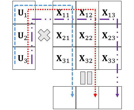
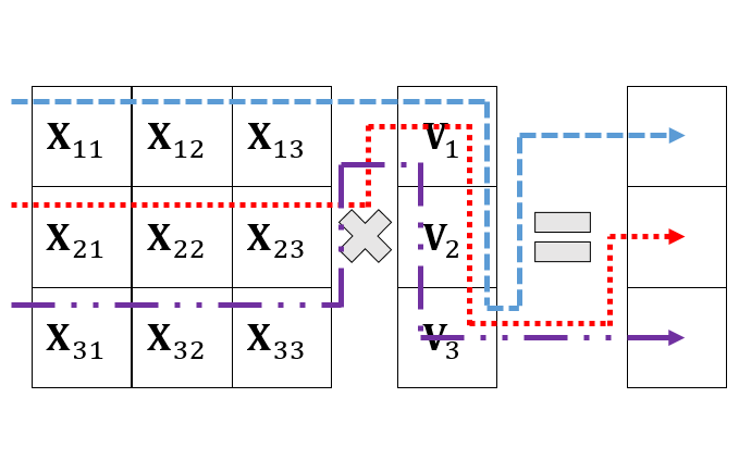
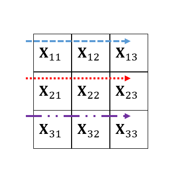
Figure 7: Parallelization of different matrix operations. Here, the number of threads \(q\) is equal to 3. Each dotted path denotes operation of a thread..
5 Parallel FaNCL for Matrix Completion↩︎
In this section, we show how the proposed algorithms can be parallelized. We will only consider the matrix completion problem in 5 . Extension to other problems, such as RPCA in Section 4.2, can be similarly performed. Moreover, for simplicity of discussion, we focus on the simpler FaNCL algorithm (Algorithm 4). Its accelerated variant (Algorithm 5) can be similarly parallelized and is shown in Appendix C.
Parallel algorithms for matrix completion have been proposed in [42]–[44]. However, they are based on stochastic gradient descent and matrix factorization, and cannot be directly used here.
5.1 Proposed Algorithm↩︎
Operations on a matrix \(\mathbf{X}\) are often of the form: (i) multiplications \(\mathbf{U}^{\top} \mathbf{X}\) and \(\mathbf{X} \mathbf{V}\) for some \(\mathbf{U}, \mathbf{V}\) (e.g., in 7 , 8 ); and (ii) element-wise operation (e.g., evaluation of \(F(\mathbf{X})\) in 4 ). A popular scheme in parallel linear algebra is block distribution [45]. Assume that there are \(q\) threads for parallelization. Block distribution partitions the rows and columns of \(\mathbf{X}\) into \(q\) parts, leading to a total of \(q^2\) blocks. For Algorithm 4, the most important variables are the low-rank factorized form \(\mathbf{U}_t \mathbf{\Sigma}_t \mathbf{V}_t^{\top}\) of \(\mathbf{X}_t\), and the sparse matrices \(\mathcal{P}_{\mathbf{\Omega}}(\mathbf{X}_t), \mathcal{P}_{\mathbf{\Omega}}(\mathbf{O})\). Using block distribution, they are simply partitioned as in \(q^2\) blocks (Figure 8). Figure 7 shows how computations of \(\mathbf{X} \mathbf{V}\), \(\mathbf{U}^{\top} \mathbf{X}\) and element-wise operation can be easily parallelized.
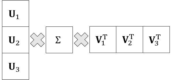

Figure 8: Partitioning of variables \(\mathbf{U} \mathbf{\Sigma} \mathbf{V}^{\top}\) and \(\mathbf{O}\), and three threads are used (\(q = 3\))..
The resultant parallelized version of FaNCL is shown in Algorithm 9. Steps that can be parallelized are marked with “\(\rhd\)”. Two new subroutines are introduced, namely, IndeSpan-PL (step 6) which replaces QR factorization, and ApproxGSVT-PL (step 9) which is the parallelized version of Algorithm 2. They will be discussed in more detail in the following Sections. Note that Algorithm 9 is equivalent to Algorithm 4 except that it is parallelized. Thus, the convergence results in Section 3.5 still hold.

5.1.1 Identifying the Span (Step 5)↩︎
In step 4 of Algorithm 4, QR factorization is used to find the span of matrix \([\mathbf{V}_t, \mathbf{V}_{t - 1}]\). This can be parallelized with the Householder transformation and Gaussian elimination [45], which however is typically very complex. The following Proposition proposes a simpler method to identify the span of a matrix.
Proposition 13. Given a matrix \(\mathbf{X}_{\text{gd}}\), let the SVD of \(\mathbf{X}_{\text{gd}} ^{\top} \mathbf{X}_{\text{gd}}\) be \(\mathbf{V} \mathbf{\Sigma} \mathbf{V}^{\top}\), \(\mathbf{w} = [w_i]\) where \(w_i = \Sigma_{ii}\) if \(\Sigma_{ii} > 0\) and \(1\) otherwise. Then, \(\mathbf{X}_{\text{gd}} \mathbf{V} \left( \text{Diag}(\mathbf{w}) \right)^{-\frac{1}{2}}\) is orthogonal and contains \(\text{span}(\mathbf{X}_{\text{gd}})\).
The resultant parallel algorithm is shown in Algorithm 10. Its time complexity is \(O( (\frac{n}{q} + q)k^2 + k^3 )\). Algorithm 9 calls Algorithm 10 with input \([\mathbf{V}_t, \mathbf{V}_{t - 1}]\), and thus takes \(O( (\frac{n}{q} + q)k_t^2 + k_t^3 )\) time, where \(k_t = r_t + r_{t - 1}\). We do not parallelize steps 2-4, as only \(k \times k\) matrices are involved and \(k\) is small. Moreover, though step 3 uses SVD, it only takes \(O(k^3)\) time.

5.1.2 Approximate GSVT (Step 8)↩︎
The key steps in approximate GSVT (Algorithm 2) are the power method and SVD. The power method can be parallelized straightforwardly as in Algorithm 11, in which we also replace the QR subroutine with Algorithm 10.
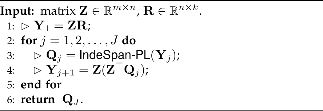
As for SVD, multiple QR factorizations are usually needed for parallelization [45], which are complex as discussed in Section 5.1.1. The following Proposition performs it in a simpler manner.
Proposition 14. Given a matrix \(\mathbf{B} \in \mathbb{R}^{n \times k}\), let \(\mathbf{P} \in \mathbb{R}^{n \times k}\) be orthogonal and equals \(\text{span}(\mathbf{B})\), and the SVD of \(\mathbf{P}^{\top} \mathbf{B}\) be \(\mathbf{U} \mathbf{\Sigma} \mathbf{V}^{\top}\). Then, the SVD of \(\mathbf{B}\) is \((\mathbf{P} \mathbf{U})\mathbf{\Sigma}\mathbf{V}\).
The resultant parallelized procedure for approximate GSVT is shown in Algorithm 12. At step 5, a small SVD is performed (by a single thread) on the \(k \times k\) matrix \(\mathbf{P}^{\top} \mathbf{B}\). At step 8 of Algorithm 9, \(\tilde{\mathbf{X}}_p\) is returned from Algorithm 12, and we keep \(\tilde{\mathbf{X}}_p\) in its low-rank factorized form. Besides, when Algorithm 12 is called, \(\mathbf{Z} = (\mathbf{X}_{\text{gd}})_t\) and has the “sparse plus low-rank” structure mentioned earlier. Hence, 7 and 8 can be used to speed up matrix multiplications3. As \(\mathbf{R}_t\) has \(k_t\) columns in Algorithm 9, PowerMethod-PL in step 1 takes \(O( \frac{k_t}{q} \| \mathbf{\Omega} \|_{1} + \frac{m + n}{q} k_t^2 )\) time, steps 2-6 take \(O( (\frac{n}{q} + q)k_t^2 + k_t^3 )\) time, and the rest takes \(O(k_t)\) time. The total time complexity for Algorithm 12 is \(O( \frac{k_t}{q} \| \mathbf{\Omega} \|_{1} + \frac{m + n}{q} k_t^2 + (q + k_t)k_t^2 )\).

5.1.3 Checking of Objectives (steps 9-11)↩︎
As shown in Figures 7 (c), computation of \(\| \mathcal{P}_{\mathbf{\Omega}}(\mathbf{X}_t - \mathbf{O}) \|_{F} ^2\) in \(F(\cdot)\) can be directly parallelized and takes \(O(\frac{1}{p}\| \mathbf{\Omega} \|_{1} )\) time. As \(r\) only relies on \(\mathbf{\Sigma}_t\), only one thread is needed to evaluate \(r(\mathbf{X}_t)\). Thus, computing \(F(\mathbf{X}_t)\) takes \(O( \frac{r_t}{q} \| \mathbf{\Omega} \|_{1} )\) time. Similarly, computing \(F( \tilde{\mathbf{X}}_p )\) takes \(O( \frac{k_t}{q} \| \mathbf{\Omega} \|_{1} )\) time. As \(\| \tilde{\mathbf{X}}_p - \mathbf{X}_t \|_{F} ^2 = \text{tr}( \tilde{\mathbf{X}}_p^{\top} \tilde{\mathbf{X}}_p - 2 \tilde{\mathbf{X}}_p^{\top} \mathbf{X}_t - \mathbf{X}_t^{\top} \mathbf{X}_t )\), the low-rank factorized forms of \(\tilde{\mathbf{X}}_p\) and \(\mathbf{X}_t\) can be utilized. From Figures 7 (a) and 7 (b), it can be performed in \(O(\frac{m + n}{q} k_t^2 )\) time. The time complexity for steps 9-11 in Algorithm 9 is \(O(\frac{k_t}{q}\| \mathbf{\Omega} \|_{1} + \frac{m + n}{q}k_t^2)\). The iteration time complexity for Algorithm 9 is thus \(O( \frac{1}{q}((m + n) k_t^2 + \| \mathbf{\Omega} \|_{1} k_t) + (q + k_t) k_t^2)\). Compared with 9 , the speedup w.r.t. the number of threads \(q\) is almost linear.
| \(m=500\) (\(12.43\%\)) | \(m=1000\) (\(6.91\%\)) | \(m=2000\) (\(3.80\%\)) | ||||||||
| NMSE | rank | time | NMSE | rank | time | NMSE | rank | time | ||
| nuclear norm | APG | 4.26\(\pm\)0.01 | 50 | 12.6\(\pm\)0.7 | 4.27\(\pm\)0.01 | 61 | 99.6\(\pm\)9.1 | 4.13\(\pm\)0.01 | 77 | 1177.5\(\pm\)134.2 |
| AIS-Impute | 4.11\(\pm\)0.01 | 55 | 5.8\(\pm\)2.9 | 4.01\(\pm\)0.03 | 57 | 37.9\(\pm\)2.9 | 3.50\(\pm\)0.01 | 65 | 338.1\(\pm\)54.1 | |
| active | 5.37\(\pm\)0.03 | 53 | 12.5\(\pm\)1.0 | 6.63\(\pm\)0.03 | 69 | 66.4\(\pm\)3.3 | 6.44\(\pm\)0.10 | 85 | 547.3\(\pm\)91.6 | |
| fixed rank | LMaFit | 3.08\(\pm\)0.02 | 5 | 0.5\(\pm\)0.1 | 3.02\(\pm\)0.02 | 5 | 1.3\(\pm\)0.1 | 2.84\(\pm\)0.03 | 5 | 4.9\(\pm\)0.3 |
| ER1MP | 21.75\(\pm\)0.05 | 40 | 0.3\(\pm\)0.1 | 21.94\(\pm\)0.09 | 54 | 0.8\(\pm\)0.1 | 20.38\(\pm\)0.06 | 70 | 2.5\(\pm\)0.3 | |
| capped \(\ell_1\) | IRNN | 1.98\(\pm\)0.01 | 5 | 14.5\(\pm\)0.7 | 1.99\(\pm\)0.01 | 5 | 146.0\(\pm\)2.6 | 1.79\(\pm\)0.01 | 5 | 2759.9\(\pm\)252.8 |
| GPG | 1.98\(\pm\)0.01 | 5 | 14.8\(\pm\)0.9 | 1.99\(\pm\)0.01 | 5 | 144.6\(\pm\)3.1 | 1.79\(\pm\)0.01 | 5 | 2644.9\(\pm\)358.0 | |
| FaNCL | 1.97\(\pm\)0.01 | 5 | 0.3\(\pm\)0.1 | 1.98\(\pm\)0.01 | 5 | 1.0\(\pm\)0.1 | 1.79\(\pm\)0.01 | 5 | 5.0\(\pm\)0.4 | |
| FaNCL-acc | 1.97\(\pm\)0.01 | 5 | 0.1\(\pm\)0.1 | 1.95\(\pm\)0.01 | 5 | 0.5\(\pm\)0.1 | 1.78\(\pm\)0.01 | 2.3\(\pm\)0.2 | ||
| LSP | IRNN | 1.96\(\pm\)0.01 | 5 | 16.8\(\pm\)0.6 | 1.89\(\pm\)0.01 | 5 | 196.1\(\pm\)3.9 | 1.79\(\pm\)0.01 | 5 | 2951.7\(\pm\)361.3 |
| GPG | 1.96\(\pm\)0.01 | 5 | 16.5\(\pm\)0.4 | 1.89\(\pm\)0.01 | 5 | 193.4\(\pm\)2.1 | 1.79\(\pm\)0.01 | 5 | 2908.9\(\pm\)358.0 | |
| FaNCL | 1.96\(\pm\)0.01 | 5 | 0.4\(\pm\)0.1 | 1.89\(\pm\)0.01 | 5 | 1.3\(\pm\)0.1 | 1.79\(\pm\)0.01 | 5 | 5.5\(\pm\)0.4 | |
| FaNCL-acc | 1.96\(\pm\)0.01 | 5 | 0.2\(\pm\)0.1 | 1.89\(\pm\)0.01 | 5 | 0.7\(\pm\)0.1 | 1.77\(\pm\)0.01 | 2.4\(\pm\)0.2 | ||
| TNN | IRNN | 1.96\(\pm\)0.01 | 5 | 18.8\(\pm\)0.6 | 1.88\(\pm\)0.01 | 5 | 223.1\(\pm\)4.9 | 1.77\(\pm\)0.01 | 5 | 3220.3\(\pm\)379.7 |
| GPG | 1.96\(\pm\)0.01 | 5 | 18.0\(\pm\)0.6 | 1.88\(\pm\)0.01 | 5 | 220.9\(\pm\)4.5 | 1.77\(\pm\)0.01 | 5 | 3197.8\(\pm\)368.9 | |
| FaNCL | 1.95\(\pm\)0.01 | 5 | 0.4\(\pm\)0.1 | 1.88\(\pm\)0.01 | 5 | 1.4\(\pm\)0.1 | 1.77\(\pm\)0.01 | 5 | 6.1\(\pm\)0.5 | |
| FaNCL-acc | 1.96\(\pm\)0.01 | 5 | 0.2\(\pm\)0.1 | 1.88\(\pm\)0.01 | 5 | 0.8\(\pm\)0.1 | 1.77\(\pm\)0.01 | 2.9\(\pm\)0.2 | ||
6 Experiments↩︎
In this section, we perform experiments on matrix completion, RPCA and the parallelized variant of Algorithm 5. We use a Windows server 2013 system with Intel Xeon E5-2695-v2 CPU (12 cores, 2.4GHz) and 256GB memory. All the algorithms in Sections 6.1 and 6.2 are implemented in Matlab. For Section 6.3, we use C++, the Intel-MKL package for matrix operations, and the standard thread library for multi-thread programming.
6.1 Matrix Completion↩︎
We compare a number of low-rank matrix completion solvers, including models based on (i) the commonly used (convex) nuclear norm regularizer; (ii) fixed-rank factorization models [40], [41], which decompose the observed matrix \(\mathbf{O}\) into a product of rank-\(k\) matrices \(\mathbf{U}\) and \(\mathbf{V}\). Its optimization problem can be written as: \(\min_{U,V}\frac{1}{2}\| \mathcal{P}_{\mathbf{\Omega}}(\mathbf{U} \mathbf{V} - \mathbf{O}) \|_{F} ^2+ \frac{\lambda}{2}(\| \mathbf{U} \|_{F} ^2 + \| \mathbf{V} \|_{F} ^2)\); and (iii) nonconvex regularizers, including the capped-\(\ell_1\) (with \(\theta\) in Table 2 set to \(2 \lambda\)), LSP (with \(\theta = \sqrt{\lambda}\)), and TNN (with \(\theta = 3\)).
The nuclear norm minimization algorithms to be compared include: (i) Accelerated proximal gradient (APG) algorithm [13], [34], with the partial SVD computed by the PROPACK package [37]; (ii) AIS-Impute [14], an inexact and accelerated proximal algorithm. The “sparse plus low-rank” structure of the matrix iterate is utilized to speed up computation (Section 4.1); and (iii) Active subspace selection (denoted “active”) [17], which adds/removes rank-one subspaces from the active set in each iteration. as they have been shown to be less efficient [15], [17]. For fixed-rank factorization models (where the rank is tuned by the validation set), we compare with the two state-of-the-art algorithms: (i) Low-rank matrix fitting (LMaFit) algorithm [40]; and (ii) Economical rank-one matrix pursuit (ER1MP) [41], which pursues a rank-one basis in each iteration. We do not compare with the concave-convex procedure [2], [18], since it has been shown to be inferior to IRNN [24]. For models with nonconvex low-rank regularizers, we compare with the following solvers: (i) Iterative reweighted nuclear norm (IRNN) [3]; (ii) Generalized proximal gradient (GPG) algorithm [26], with the underlying problem (?? ) solved using the closed-form solutions in [24]; and (iii) The proposed FaNCL algorithm (Algorithm 4) and its accelerated variant FaNCL-acc (Algorithm 5). We set \(J = 3\) and \(p = 1\).
All the algorithms are stopped when the relative difference in objective values between consecutive iterations is smaller than \({10}^{-4}\).
6.1.1 Synthetic Data↩︎
The observed \(m\times m\) matrix is generated as \(\mathbf{O} = \mathbf{U} \mathbf{V} + \mathbf{G}\), where the elements of \(\mathbf{U} \in \mathbb{R}^{m \times k}, \mathbf{V} \in \mathbb{R}^{k \times m}\) (with \(k = 5\)) are sampled i.i.d. from the standard normal distribution \(\mathcal{N}(0, 1)\), and elements of \(\mathbf{G}\) sampled from \(\mathcal{N}(0, 0.1)\). A total of \(\| \mathbf{\Omega} \|_{1} = 2 m k \log(m)\) random elements in \(\mathbf{O}\) are observed. Half of them are used for training, and the rest as validation set for parameter tuning. Testing is performed on the unobserved elements.
For performance evaluation, we use (i) the normalized mean squared error: \(\text{NMSE} = \| P_{\mathbf{\Omega}^{\bot}}(\mathbf{X} - \mathbf{U V}) \|_{F} / \| P_{\mathbf{\Omega}^{\bot}}(\mathbf{U V}) \|_{F}\), where \(\mathbf{X}\) is the recovered matrix and \(\mathbf{\Omega}^{\bot}\) denotes the unobserved positions; (ii) rank of \(\mathbf{X}\); and (iii) training CPU time. We vary \(m\) in \(\{500, 1000, 2000\}\). Each experiment is repeated five times.
Results are shown in 4 Table 4. As can be seen, nonconvex regularization (capped-\(\ell_1\), LSP and TNN) leads to much lower NMSE’s than convex nuclear norm regularization and fixed-rank factorization. Moreover, nuclear norm regularization and ER1MP produce much higher ranks. In terms of speed among the nonconvex low-rank solvers, FaNCL is faster than GPG and IRNN, while FaNCL-acc is even faster. Moreover, the larger the matrix, the higher are the speedups of FaNCL and FaNCL-acc over GPG and IRNN.
Next, we demonstrate the ability of FaNCL and FaNCL-acc in maintaining low-rank iterates. Figure 13 shows \(k\) (the rank of \(\mathbf{R}_t\)) and \(\hat{k}_{\mathbf{X}_+}\) (the rank of \(\mathbf{X}_{t + 1}\)) vs the number of iterations for \(m=500\). As can be seen, \(k \ge \hat{k}_{\mathbf{X}_{\text{gd}}}\), which agrees with the assumption in Proposition 5. Besides, as FaNCL/FaNCL-acc converges, \(k\) and \(\hat{k}_{\mathbf{X}_{\text{gd}}}\) gradually converge to the same value. Moreover, recall that the data matrix is of size \(500 \times 500\). Hence, the ranks of the iterates obtained by both algorithms are low.


Figure 13: \(k\) and \(\hat{k}_{\mathbf{X}_{\text{gd}}}\) vs the number of iterations on the synthetic data set with \(m = 500\). The plot of TNN is similar and thus not shown..
6.1.2 Recommendation Data sets↩︎
MovieLens: First, we perform experiments on the popular MovieLens data set (Table 5), which contain ratings of different users on movies. We follow the setup in [41], and use \(50\%\) of the observed ratings for training, \(25\%\) for validation and the rest for testing. For performance evaluation, we use the root mean squared error on the test set \(\bar{\mathbf{\Omega}}\): \(\text{RMSE} = \sqrt{ \| \mathcal{P}_{\bar{\mathbf{\Omega}}}(\mathbf{X} - \mathbf{O}) \|_{F} ^2 / \| \mathbf{\bar{\Omega}} \|_{1} }\), where \(\mathbf{X}\) is the recovered matrix. The experiment is repeated five times.
| #users | #movies | #ratings | ||
|---|---|---|---|---|
| MovieLens | 100K | 943 | 1,682 | 100,000 |
| 1M | 6,040 | 3,449 | 999,714 | |
| 10M | 69,878 | 10,677 | 10,000,054 | |
| netflix | 480,189 | 17,770 | 100,480,507 | |
| yahoo | 249,012 | 296,111 | 62,551,438 | |
Results are shown in Table 6. Again, nonconvex regularizers lead to the lowest RMSE’s. Moreover, FaNCL-acc is also the fastest among nonconvex low-rank solvers, even faster than the state-of-the-art GPG. In particular, FaNCL and its accelerated variant FaNCL-acc are the only solvers (for nonconvex regularization) that can be run on the MovieLens-1M and 10M data sets. Figure 14 compares the objectives vs CPU time for the nonconvex regularization solvers on MovieLens-100K. As can be seen, FaNCL and FaNCL-acc decrease the objective and RMSE much faster than the others. Figure 15 shows the testing RMSEs on MovieLens-1M and 10M. As can be seen, FaNCL-acc is the fastest.
| MovieLens-100K | MovieLens-1M | MovieLens-10M | netflix | yahoo | |||||||
| RMSE | rank | RMSE | rank | RMSE | rank | RMSE | rank | RMSE | rank | ||
| nuclear | APG | 0.877\(\pm\)0.001 | 36 | 0.818\(\pm\)0.001 | 67 | — | — | — | — | — | — |
| norm | AIS-Impute | 0.878\(\pm\)0.002 | 36 | 0.819\(\pm\)0.001 | 67 | 0.813\(\pm\)0.001 | 100 | — | — | — | — |
| active | 0.878\(\pm\)0.001 | 36 | 0.820\(\pm\)0.001 | 67 | 0.814\(\pm\)0.001 | 100 | — | — | — | — | |
| fixed | LMaFit | 0.865\(\pm\)0.002 | 2 | 0.806\(\pm\)0.003 | 6 | 0.792\(\pm\)0.001 | 9 | 0.811\(\pm\)0.001 | 15 | 0.666\(\pm\)0.001 | 10 |
| rank | ER1MP | 0.917\(\pm\)0.003 | 5 | 0.853\(\pm\)0.001 | 13 | 0.852\(\pm\)0.002 | 22 | 0.862\(\pm\)0.006 | 25 | 0.810\(\pm\)0.003 | 77 |
| capped | IRNN | 0.854\(\pm\)0.003 | 3 | — | — | — | — | — | — | — | — |
| \(\ell_1\) | GPG | 0.855\(\pm\)0.002 | 3 | — | — | — | — | — | — | — | — |
| FaNCL | 0.855\(\pm\)0.003 | 3 | 0.788\(\pm\)0.002 | 5 | 0.783\(\pm\)0.001 | 8 | 0.798\(\pm\)0.001 | 13 | 0.656\(\pm\)0.001 | 8 | |
| FaNCL-acc | 0.860\(\pm\)0.009 | 3 | 0.791\(\pm\)0.001 | 5 | 0.778\(\pm\)0.001 | 8 | 0.795\(\pm\)0.001 | 13 | 0.651\(\pm\)0.001 | 8 | |
| LSP | IRNN | 0.856\(\pm\)0.001 | 2 | — | — | — | — | — | — | — | — |
| GPG | 0.856\(\pm\)0.001 | 2 | — | — | — | — | — | — | — | — | |
| FaNCL | 0.856\(\pm\)0.001 | 2 | 0.786\(\pm\)0.001 | 5 | 0.779\(\pm\)0.001 | 9 | 0.794\(\pm\)0.001 | 15 | 0.652\(\pm\)0.001 | 9 | |
| FaNCL-acc | 0.853\(\pm\)0.001 | 2 | 0.787\(\pm\)0.001 | 5 | 0.779\(\pm\)0.001 | 9 | 0.792\(\pm\)0.001 | 15 | 0.650\(\pm\)0.001 | 8 | |
| TNN | IRNN | 0.854\(\pm\)0.004 | 3 | — | — | — | — | — | — | — | — |
| GPG | 0.853\(\pm\)0.005 | 3 | — | — | — | — | — | — | — | — | |
| FaNCL | 0.865\(\pm\)0.016 | 3 | 0.786\(\pm\)0.001 | 5 | 0.780\(\pm\)0.001 | 8 | 0.797\(\pm\)0.001 | 13 | 0.657\(\pm\)0.001 | 7 | |
| FaNCL-acc | 0.861\(\pm\)0.009 | 3 | 0.786\(\pm\)0.001 | 5 | 0.778\(\pm\)0.001 | 9 | 0.795\(\pm\)0.001 | 13 | 0.650\(\pm\)0.001 | 7 | |


Figure 14: Objective vs CPU time for the capped-\(\ell_1\) and LSP on MovieLens-100K. The plot of TNN is similar and thus not shown..

Figure 15: RMSE vs CPU time on the MovieLens-1M and 10M data sets..
Figure 16 shows the ranks \(k\) and \(\hat{k}_{\mathbf{X}_{\text{gd}}}\) (as defined in Proposition 5) vs the number of iterations on the MovieLens-100K data set. Recall that the data matrix is of size \(943 \times 1682\). Again, \(k \ge \hat{k}_{\mathbf{X}_{\text{gd}}}\) and the ranks of the iterates obtained by both algorithms are low.


Figure 16: \(k\) and \(\hat{k}_{\mathbf{X}_{\text{gd}}}\) vs the number of iterations on the MovieLens-100K data set. The plot of TNN is similar and thus not shown..
Netflix and Yahoo: Next, we perform experiments on two very large recommendation data sets, Netflix and Yahoo (Table 5). We randomly use \(50\%\) of the observed ratings for training, \(25\%\) for validation and the rest for testing. Each experiment is repeated five times.
Results are shown in Table 6. APG, GPG and IRNN cannot be run as the data set is large. From Section 6.1.2, AIS-Impute has similar running time as LMaFit but inferior performance, and thus is not compared. Again, the nonconvex regularizers converge faster, yield lower RMSE’s and solutions of much lower ranks. Figure 17 shows the RMSE vs time, and FaNCL-acc is the fastest.


Figure 17: RMSE vs CPU time on the netflix and yahoo data sets..
| tree | rice | wall | ||||||||
| RMSE | rank | time | RMSE | rank | time | RMSE | rank | time | ||
| nuclear | APG | 0.433\(\pm\)0.001 | 180 | 308.7\(\pm\)71.9 | 0.224\(\pm\)0.002 | 148 | 242.3\(\pm\)27.8 | 0.222\(\pm\)0.001 | 165 | 311.5\(\pm\)31.2 |
| norm | AIS-Impute | 0.432\(\pm\)0.001 | 181 | 251.6\(\pm\)61.7 | 0.225\(\pm\)0.002 | 150 | 138.1\(\pm\)5.7 | 0.223\(\pm\)0.001 | 168 | 156.6\(\pm\)11.1 |
| active | 0.445\(\pm\)0.001 | 222 | 935.5\(\pm\)117.9 | 0.263\(\pm\)0.002 | 170 | 640.8\(\pm\)10.8 | 0.258\(\pm\)0.001 | 189 | 739.1\(\pm\)61.8 | |
| fixed | LMaFit | 0.518\(\pm\)0.012 | 9 | 5.4\(\pm\)1.1 | 0.281\(\pm\)0.031 | 10 | 7.8\(\pm\)1.6 | 0.229\(\pm\)0.006 | 10 | 9.2\(\pm\)2.1 |
| rank | ER1MP | 0.473\(\pm\)0.001 | 19 | 1.5\(\pm\)0.2 | 0.295\(\pm\)0.002 | 22 | 2.2\(\pm\)0.6 | 0.269\(\pm\)0.003 | 20 | 1.2\(\pm\)0.1 |
| LSP | IRNN | 0.416\(\pm\)0.003 | 12 | 204.9\(\pm\)19.0 | 0.197\(\pm\)0.003 | 15 | 480.0\(\pm\)50.5 | 0.196\(\pm\)0.001 | 17 | 562.5\(\pm\)0.8 |
| GPG | 0.417\(\pm\)0.004 | 12 | 195.9\(\pm\)17.5 | 0.197\(\pm\)0.003 | 15 | 464.3\(\pm\)55.0 | 0.195\(\pm\)0.001 | 17 | 557.6\(\pm\)17.1 | |
| FaNCL | 0.416\(\pm\)0.002 | 12 | 10.6\(\pm\)1.8 | 0.198\(\pm\)0.004 | 15 | 25.0\(\pm\)1.8 | 0.199\(\pm\)0.005 | 17 | 27.5\(\pm\)1.0 | |
| FaNCL-acc | 0.414\(\pm\)0.001 | 12 | 5.4\(\pm\)0.8 | 0.197\(\pm\)0.001 | 15 | 8.4\(\pm\)1.2 | 0.194\(\pm\)0.001 | 17 | 11.7\(\pm\)0.6 | |
6.1.3 Image Data Sets↩︎
Grayscale Images: We use the images in [2] (Figures 18). The pixels are normalized to zero mean and unit variance. Gaussian noise from \(\mathcal{N}(0, 0.05)\) is then added. In each image, 20% of the pixels are randomly sampled as observations (half for training and the half for validation). The task is to fill in the remaining 80% of the pixels. The experiment is repeated five times. The LSP regularizer is used, as it usually has comparable or better performance than the capped-\(\ell_1\) and TNN regularizers (as can be seen from Sections 6.1.1 and 6.1.2). The experiment is repeated five times.


Figure 18: Grayscale images used in the experiment..
Table 7 shows the testing RMSE, rank obtained, and running time. As can be seen, models based on low-rank factorization (LMaFit and ER1MP) and nuclear norm regularization (AIS-Impute) have higher testing RMSE’s than those using LSP regularization (IRNN, GPG, FaNCL, and FaNCL-acc). Figure 19 shows convergence of the testing RMSE. Among the LSP regularization algorithms, FaNCL-acc is the fastest, which is then followed by FaNCL, GPG, and IRNN.


Figure 19: Testing RMSE vs CPU time (in seconds) on the grayscale images. The plot of wall is similar and thus not shown..
Hyperspectral Images: In this experiment, hyperspectral images (Figure 20) are used. Each sample is a \(I_1 \times I_2 \times I_3\) tensor, where \(I_1\times I_2\) is the image size, and \(I_3\) is the number of frequencies used to scan the object. As in [46], we convert this to a \(I_1 I_2 \times I_3\) matrix. The pixels are normalized to zero mean and unit variance, and Gaussian noise from \(\mathcal{N}(0, 0.05)\) is added. 1% of the pixels are randomly sampled for training, 0.5% for validation and the remaining for testing. Again, we use the LSP regularizer. The experiment is repeated five times. As IRNN and GPG are slow (Sections 6.1.1 and 6.1.2), while APG and active subspace selection have been shown to be inferior to AIS-Impute on the greyscale images, they will not be compared here.


Figure 20: Hyperspectral images used in the experiment, their sizes are 1312\(\times\)480\(\times\)49, 1312\(\times\)528\(\times\)49 and 1312\(\times\)480\(\times\)49, respectively. One sample band of each image is shown..
Table 8 shows the testing RMSE, rank obtained and running time. As on grayscale images, FaNCL and FaCNL-acc have lower testing RMSE’s than models based on low-rank factorization (LMaFit and ER1MP) and nuclear norm regularization (AIS-Impute). Figure 21 shows convergence of the testing RMSE. Again, FaNCL-acc is much faster than FaNCL.


Figure 21: Testing RMSE vs CPU time (in seconds) on the hyperspectral images. The plot of corn is similar and thus not shown..
| broccoli | cabbage | corn | ||||||||
| RMSE | rank | time | RMSE | rank | time | RMSE | rank | time | ||
| nuclear norm | AIS-Impute | 0.275\(\pm\)0.001 | 34 | 560\(\pm\)90 | 0.180\(\pm\)0.001 | 28 | 493\(\pm\)46 | 0.236\(\pm\)0.001 | 41 | 519.1\(\pm\)94.7 |
| fixed rank | LMaFit | 0.302\(\pm\)0.001 | 2 | 6\(\pm\)2 | 0.181\(\pm\)0.001 | 3 | 6\(\pm\)3 | 0.265\(\pm\)0.002 | 5 | 3/9\(\pm\)1.5 |
| ER1MP | 0.344\(\pm\)0.002 | 21 | 88\(\pm\)12 | 0.252\(\pm\)0.003 | 41 | 75\(\pm\)23 | 0.299\(\pm\)0.004 | 37 | 55.4\(\pm\)7.2 | |
| LSP | FaNCL | 0.252\(\pm\)0.003 | 9 | 6079\(\pm\)1378 | 0.149\(\pm\)0.001 | 10 | 3243\(\pm\)163 | 0.204\(\pm\)0.004 | 15 | 4672.8\(\pm\)967.8 |
| FaNCL-acc | 0.251\(\pm\)0.004 | 9 | 274\(\pm\)77 | 0.149\(\pm\)0.001 | 10 | 221\(\pm\)12 | 0.203\(\pm\)0.002 | 15 | 273.8\(\pm\)75.4 | |
6.2 Robust Principal Component Analysis↩︎
6.2.1 Synthetic Data↩︎
In this section, we first perform experiments on a synthetic data set. The observed \(m \times m\) matrix is generated as \(\mathbf{O} = \mathbf{U} \mathbf{V} + \tilde{\mathbf{S}} + \mathbf{G}\), where elements of \(\mathbf{U} \in \mathbb{R}^{m \times k}, \mathbf{V} \in \mathbb{R}^{k \times m}\) (with \(k = 0.01m\)) are sampled i.i.d. from \(\mathcal{N}(0, 1)\), and elements of \(\mathbf{G}\) are sampled from \(\mathcal{N}(0, 0.1)\). Matrix \(\tilde{\mathbf{S}}\) is sparse, with \(1\%\) of its elements randomly set to \(5 \| \mathbf{U} \mathbf{V} \|_{\infty}\) or \(- 5 \| \mathbf{U} \mathbf{V} \|_{\infty}\) with equal probabilities. The columns of \(\mathbf{O}\) is then randomly split into training and test sets of equal size. The standard \(\ell_1\) regularizer is used as the sparsity regularizer \(g\) in (10 ), and different convex/nonconvex low-rank regularizers are used as \(r\). Hyperparameters \(\lambda\) and \(\upsilon\) in 10 are tuned using the training set.
| \(m=500\) | \(m=1000\) | \(m=2000\) | ||||||||
| NMSE | rank | time | NMSE | rank | time | NMSE | rank | time | ||
| nuclear norm | APG | 4.88\(\pm\)0.17 | 5 | 4.3\(\pm\)0.2 | 3.31\(\pm\)0.06 | 10 | 24.5\(\pm\)1.0 | 2.40\(\pm\)0.05 | 20 | 281.2\(\pm\)26.7 |
| capped-\(\ell_1\) | GPG | 4.51\(\pm\)0.16 | 5 | 8.5\(\pm\)2.6 | 2.93\(\pm\)0.07 | 10 | 42.9\(\pm\)6.6 | 2.16\(\pm\)0.05 | 20 | 614.1\(\pm\)64.7 |
| FaNCL-acc | 4.51\(\pm\)0.16 | 5 | 0.8\(\pm\)0.2 | 2.93\(\pm\)0.07 | 10 | 2.8\(\pm\)0.1 | 2.16\(\pm\)0.05 | 20 | 24.9\(\pm\)2.0 | |
| LSP | GPG | 4.51\(\pm\)0.16 | 5 | 8.3\(\pm\)2.3 | 2.93\(\pm\)0.07 | 10 | 42.6\(\pm\)5.9 | 2.16\(\pm\)0.05 | 20 | 638.8\(\pm\)72.6 |
| FaNCL-acc | 4.51\(\pm\)0.16 | 5 | 0.8\(\pm\)0.1 | 2.93\(\pm\)0.07 | 10 | 2.9\(\pm\)0.1 | 2.16\(\pm\)0.05 | 20 | 26.6\(\pm\)4.1 | |
| TNN | GPG | 4.51\(\pm\)0.16 | 5 | 8.5\(\pm\)2.4 | 2.93\(\pm\)0.07 | 10 | 43.2\(\pm\)5.8 | 2.16\(\pm\)0.05 | 20 | 640.7\(\pm\)59.1 |
| FaNCL-acc | 4.51\(\pm\)0.16 | 5 | 0.8\(\pm\)0.1 | 2.93\(\pm\)0.07 | 10 | 2.9\(\pm\)0.1 | 2.16\(\pm\)0.05 | 20 | 26.9\(\pm\)2.7 | |
For performance evaluation, we use the (i) testing NMSE \(=\| (\mathbf{X}+ \mathbf{S}) - \mathcal{P}_{\mathcal{T}}(\mathbf{UV+\tilde{S}}) \|_{F} / \| \mathcal{P}_{\mathcal{T}}(\mathbf{UV+\tilde{S}} ) \|_{F}\), where \(\mathcal{T}\) indices columns in the test set, \(\mathbf{X}\) and \(\mathbf{S}\) are the recovered low-rank and sparse components, respectively; (ii) accuracy on locating the sparse support of \(\tilde{\mathbf{S}}\) (i.e., percentage of entries that \(\tilde{S}_{ij}\) and \(S_{ij}\) are nonzero or zero together); (iii) the recovered rank and (iv) CPU time. We vary \(m\) in \(\{500, 1000, 2000\}\). Each experiment is repeated five times. Note that IRNN and active subspace selection cannot be used here. Their objectives are of the form “smooth function plus low-rank regularizer", but RPCA also has a nonsmooth \(\ell_1\) regularizer. Similarly, AIS-Impute is only for matrix completion. Moreover, FaNCL, which has been shown to be slower than FaNCL-acc, will not be compared.
Results are shown in Table 9. The accuracies on locating the sparse support are always 100% for all methods, and thus are not shown. Moreover, while both convex and nonconvex regularizers can perfectly recover the matrix rank and sparse locations, the nonconvex regularizers have lower NMSE’s. As in matrix completion, FaNCL-acc is much faster. The larger the matrix, the higher the speedup.
6.2.2 Background Removal in Videos↩︎
In this section, we use RPCA for background removal in videos. Four benchmark videos in [5], [6] are used (Table 10), and example frames are shown in Figure 22. As in [5], the image background is considered low-rank, while the foreground moving objects contribute to the sparse component.
| bootstrap | campus | escalator | hall | |
|---|---|---|---|---|
| #pixels / frame | 19,200 | 20,480 | 20,800 | 25,344 |
| total #frames | 9,165 | 4,317 | 10,251 | 10,752 |


Figure 22: Example image frames in the videos..
| bootstrap | campus | escalator | hall | ||||||
| PSNR | time | PSNR | time | PSNR | time | PSNR | time | ||
| nuclear norm | APG | 23.07\(\pm\)0.02 | 524\(\pm\)84 | 22.47\(\pm\)0.02 | 101\(\pm\)6 | 24.01\(\pm\)0.01 | 594\(\pm\)86 | 24.25\(\pm\)0.03 | 553\(\pm\)85 |
| capped-\(\ell_1\) | GPG | 23.81\(\pm\)0.01 | 3122\(\pm\)284 | 23.21\(\pm\)0.02 | 691\(\pm\)43 | 24.62\(\pm\)0.02 | 5369\(\pm\)238 | 25.22\(\pm\)0.03 | 4841\(\pm\)255 |
| FaNCL-acc | 24.05\(\pm\)0.01 | 193\(\pm\)18 | 23.24\(\pm\)0.02 | 53\(\pm\)5 | 24.68\(\pm\)0.02 | 242\(\pm\)22 | 25.22\(\pm\)0.03 | 150\(\pm\)10 | |
| LSP | GPG | 23.93\(\pm\)0.03 | 1922\(\pm\)111 | 23.61\(\pm\)0.02 | 324\(\pm\)27 | 24.57\(\pm\)0.01 | 5053\(\pm\)369 | 25.37\(\pm\)0.03 | 2889\(\pm\)222 |
| FaNCL-acc | 24.30\(\pm\)0.02 | 189\(\pm\)15 | 23.99\(\pm\)0.02 | 69\(\pm\)8 | 24.56\(\pm\)0.01 | 168\(\pm\)15 | 25.37\(\pm\)0.03 | 144\(\pm\)9 | |
| TNN | GPG | 23.85\(\pm\)0.03 | 1296\(\pm\)203 | 23.12\(\pm\)0.02 | 671\(\pm\)21 | 24.60\(\pm\)0.01 | 4091\(\pm\)195 | 25.26\(\pm\)0.04 | 4709\(\pm\)367 |
| FaNCL-acc | 24.12\(\pm\)0.02 | 203\(\pm\)11 | 23.14\(\pm\)0.02 | 49\(\pm\)5 | 24.66\(\pm\)0.01 | 254\(\pm\)30 | 25.25\(\pm\)0.06 | 148\(\pm\)11 | |
Given a video with \(n\) image frames, each \(m_1 \times m_2\) frame is first reshaped as a \(m\)-dimensional column vector (where \(m = m_1 m_2\)), and then all the frames are stacked together to form a \(m \times n\) matrix. The pixel values are normalized to \([0, 1]\), and Gaussian noise from \(\mathcal{N}(0, 0.15)\) is added. The experiment is repeated five times. For performance evaluation, we use the commonly used peak signal-to-noise ratio [4]: PSNR \(= - 10 \log_{10}(\frac{1}{m n} \| \mathbf{X} - \mathbf{O} \|_{F} ^2)\) where \(\mathbf{X} \in \mathbb{R}^{m \times n}\) is the recovered video, and \(\mathbf{O} \in \mathbb{R}^{m \times n}\) is the ground-truth.
Results are shown in Table 11. As can be seen, the nonconvex regularizers lead to better PSNR’s than the convex nuclear norm. Moreover, FaNCL-acc is much faster than GPG. Figure 23 shows PSNR vs CPU time on the bootstrap and campus data sets. Again, FaNCL-acc converges to higher PSNR much faster. Results on hall and escalator are similar.


Figure 23: PSNR vs CPU time on the bootstrap and campus videos..
6.3 Parallel Matrix Completion↩︎
In this section, we experiment with the proposed parallel algorithm in Section 5 on the Netflix and Yahoo data sets (Table 5). We do not compare with factorization-based algorithms [43], [44], as they have inferior performance (Section 6.1). The machine has 12 cores, and one thread is used for each core. As suggested in [43], we randomly shuffle all the matrix columns and rows before partitioning. We use the LSP penalty (with \(\theta = \sqrt{\lambda}\)) and fix the total number of iterations to 250. The hyperparameters are the same as in Section 6.1.2. Experiments are repeated five times.
Convergence of the objective for a typical run is shown in Figure 24. As we have multiple threads running on a single CPU, we report the clock time instead of CPU time. As can be seen, the accelerated algorithms are much faster than the non-accelerated ones, and parallelization provides further speedup.
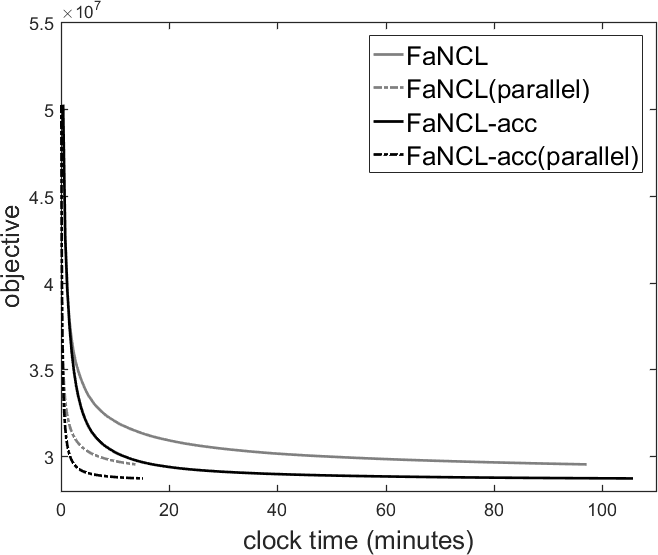

Figure 24: Objective value vs clock time for the sequential/parallel versions of FaNCL on the netflix and yahoo data sets..
Figure 25 (a) shows the per-iteration clock time with different numbers of threads. As can be seen, the clock time decreases significantly with the number of threads. Note that the curves for FaNCL and FaNCL-acc overlap. This is because of the per-iteration time complexity of FaNCL-acc is only slightly higher than that of FaNCL (Section 3.6). Figure 25 (b) shows the speedup with different numbers of threads. In particular, scaling is better on yahoo. The observed entries in its partitioned data submatrices are distributed more evenly, which improves performance of parallel algorithms [42]. Another observation is that the speedup can be larger than one. As discussed in [45], in performing multiplications with a large sparse matrix, a significant amount of time is spent on indexing its nonzero elements. When the matrix is partitioned, each submatrix becomes smaller and easier to be indexed. Thus, the memory cache also becomes more effective.


Figure 25: Clock time (seconds) per iteration and speedup vs the number of threads for parallel FaNCL. The dashed line in Figure 25 (b) corresponds to linear speedup..
7 Conclusion↩︎
In this paper, we considered the challenging problem of nonconvex low-rank matrix optimization. The key observations are that for the popular low-rank regularizers, the singular values obtained from the proximal operator can be automatically thresholded, and the proximal operator can be computed on a smaller matrix. This allows the proximal operator to be efficiently approximated by the power method. We extended the proximal algorithm in this nonconvex optimization setting with acceleration and inexact proximal step. We further parallelized the proposed algorithm, which scales well w.r.t. the number of threads. Extensive experiments on matrix completion and RPCA show that the proposed algorithm is much faster than the state-of-the-art. It also demonstrates that nonconvex low-rank regularizers outperform the standard (convex) nuclear norm regularizer.
Acknowledgment↩︎
This research was supported in part by the Research Grants Council of the Hong Kong Special Administrative Region (Grant 614513), Microsoft Research Asia and 4Paradigm.
References↩︎
All Proofs are in Appendix A.↩︎
We noticed a similar result in [35] after the conference version of this paper [36] has been accepted. However, [35] only considers the case where \(r\) is the nuclear norm regularizer.↩︎
As no acceleration is used, \(\beta_t\) in 7 and 8 is equal to zero in these two equations.↩︎
For all tables in the sequel, the best and comparable results (according to the pairwise t-test with 95% confidence) are highlighted.↩︎